Unsupervised Multi-Object Detection for Video Surveillance Using Memory-Based Recurrent Attention Networks


Abstract
:1. Introduction
- We propose an Unsupervised Multi-Object Detection (UMOD) framework, where a neural model learns to detect objects from each video frame by minimizing the image reconstruction error.
- We propose aMemory-Based Recurrent Attention Network to improve detection efficiency and ease model training.
- We assess the proposed model on both the synthetic dataset (Sprites) and the real dataset (DukeMTMC [17]), exhibiting its advantages and practicality.
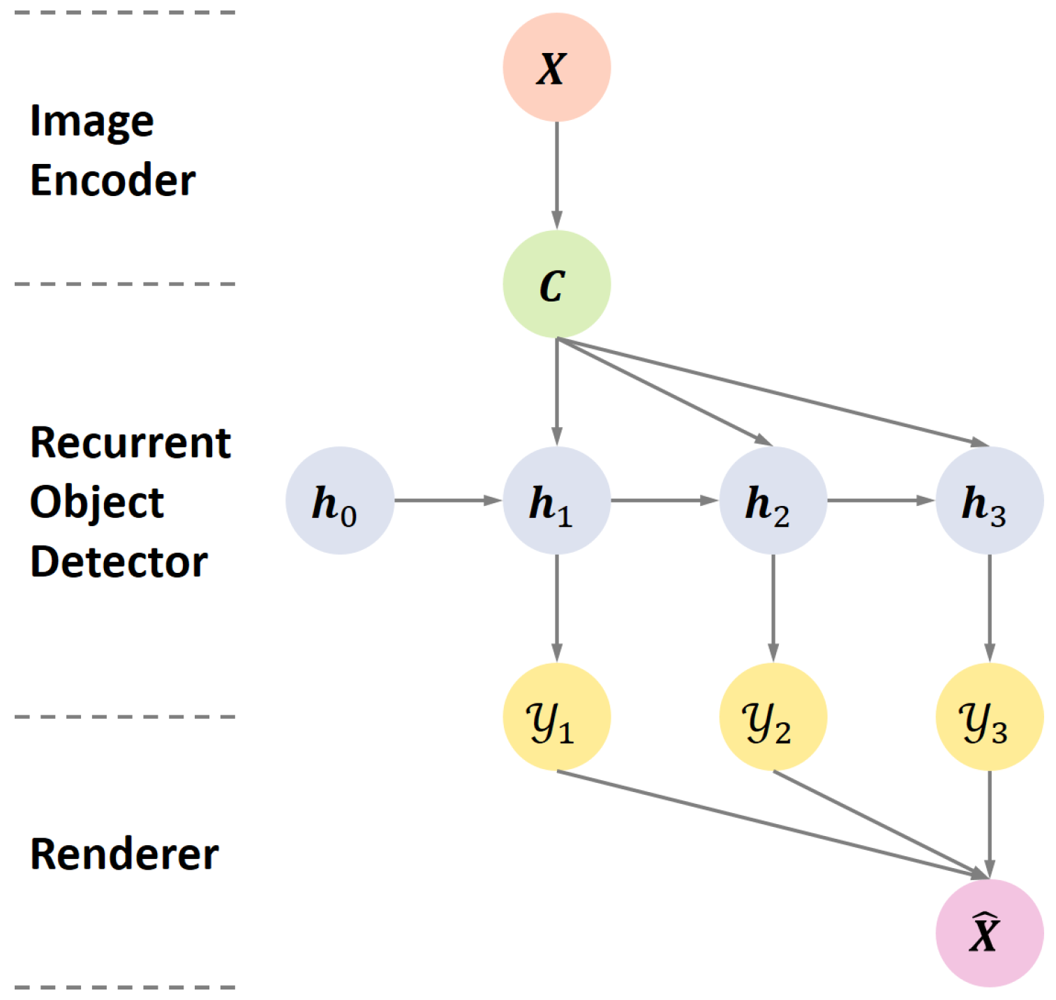
2. Unsupervised Multi-Object Detection
2.1. Image Encoder
2.2. Recurrent Object Detector
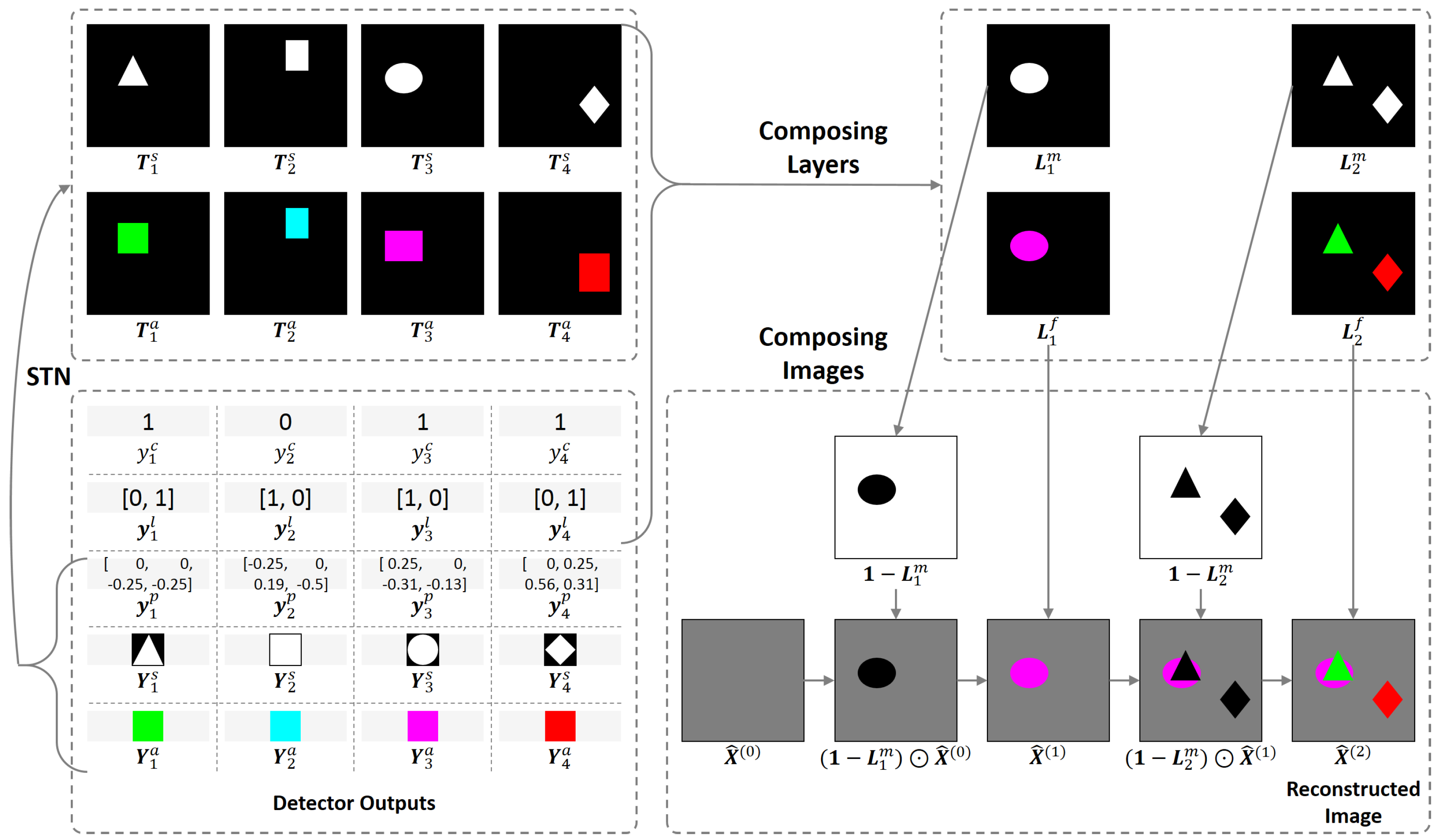
2.3. Renderer
2.4. Loss
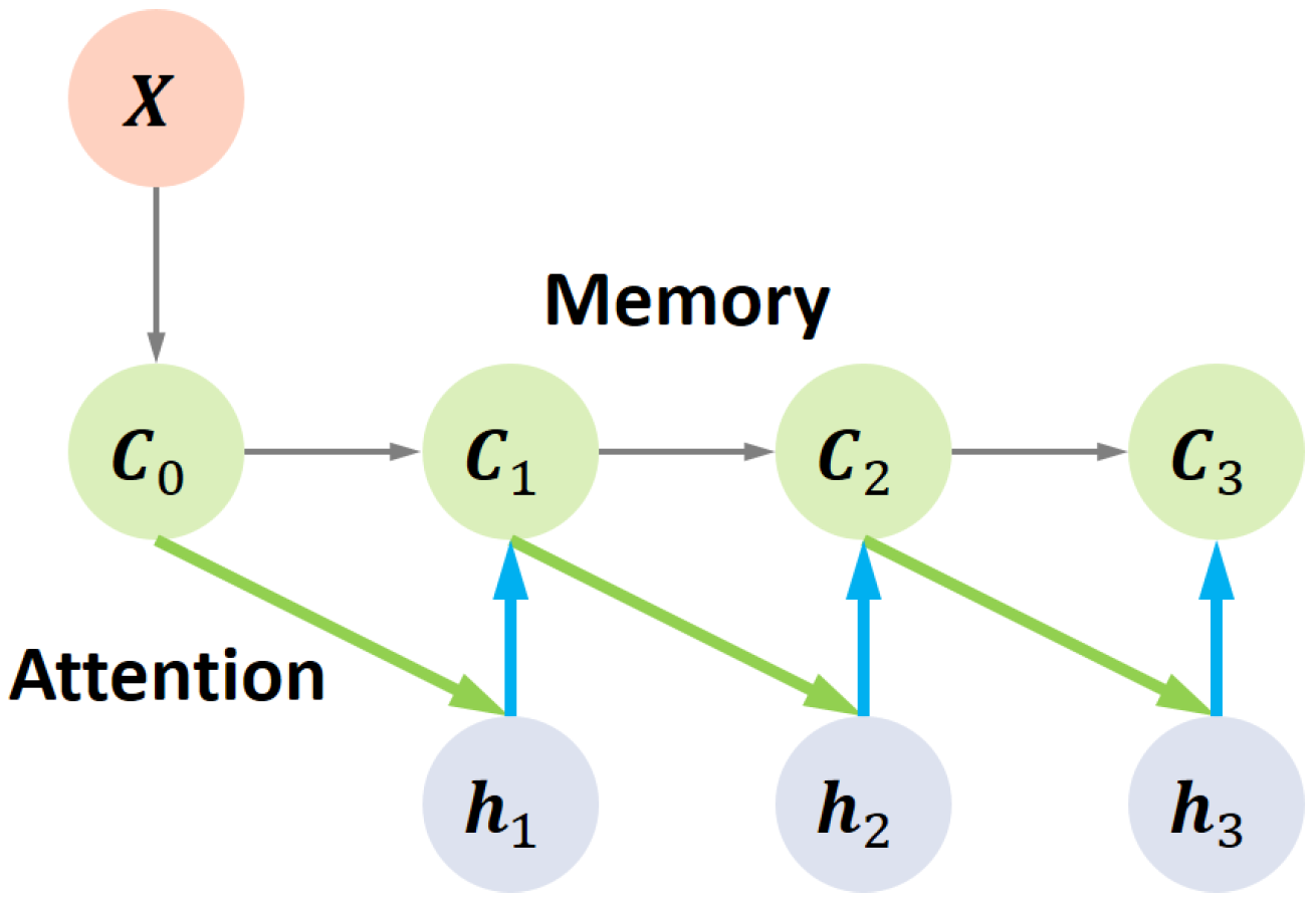
3. Memory-Based Recurrent Attention Networks
4. Experiments
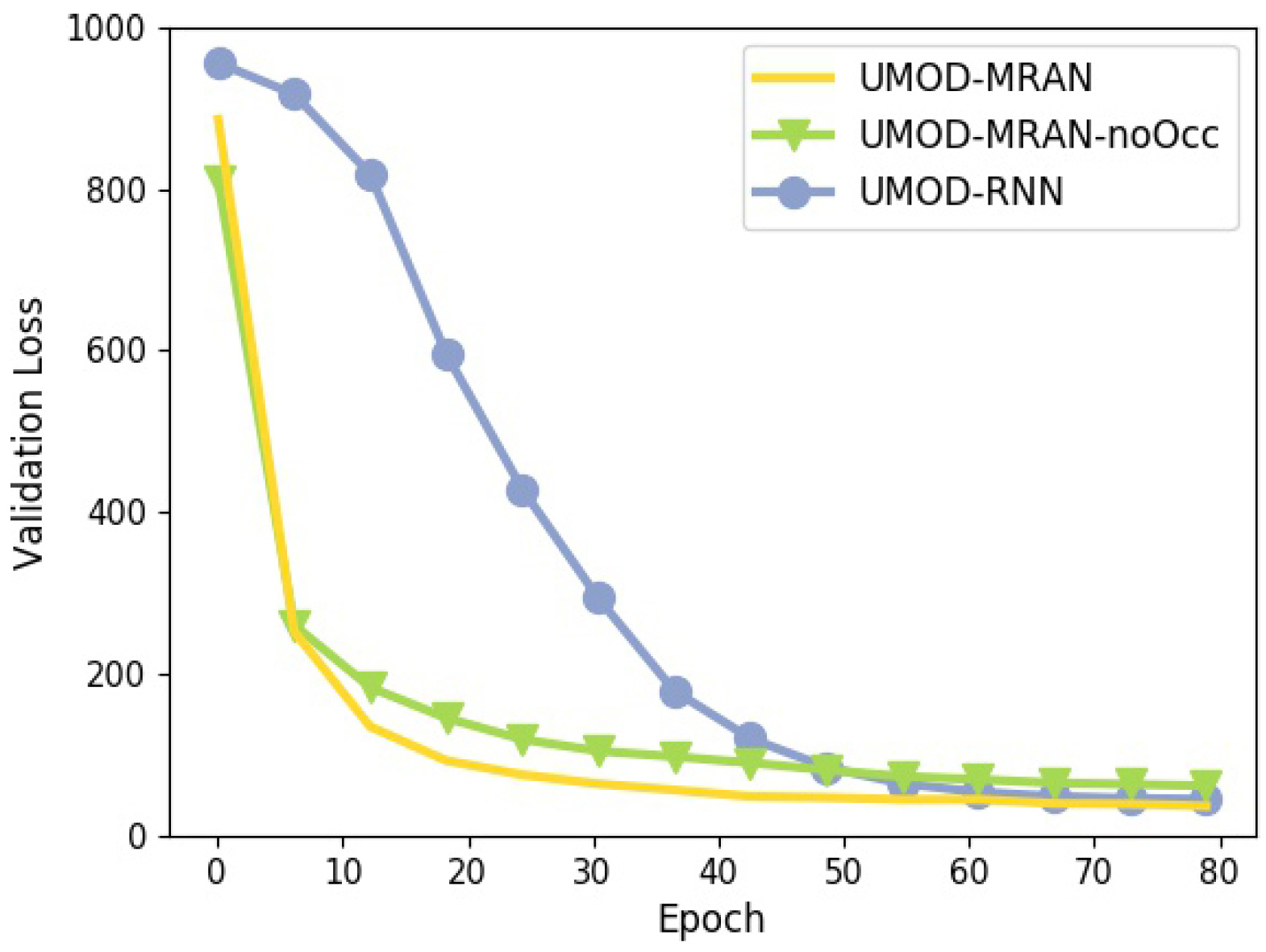
- UMOD-MRAN-noOcc. UMOD-MRAN without occlusion reasoning, which is achieved by fixing the layer number I to 1.
- UMOD-RNN. UMOD with RNN, which is achieved by setting the recurrent module as a Gated Recurrent Unit [20] as described in Section 2.2, thereby disabling the external memory and attention.
- AIR. Our implementation of the generative model proposed in [26] that could be used for MOD through inference.
4.1. Sprites
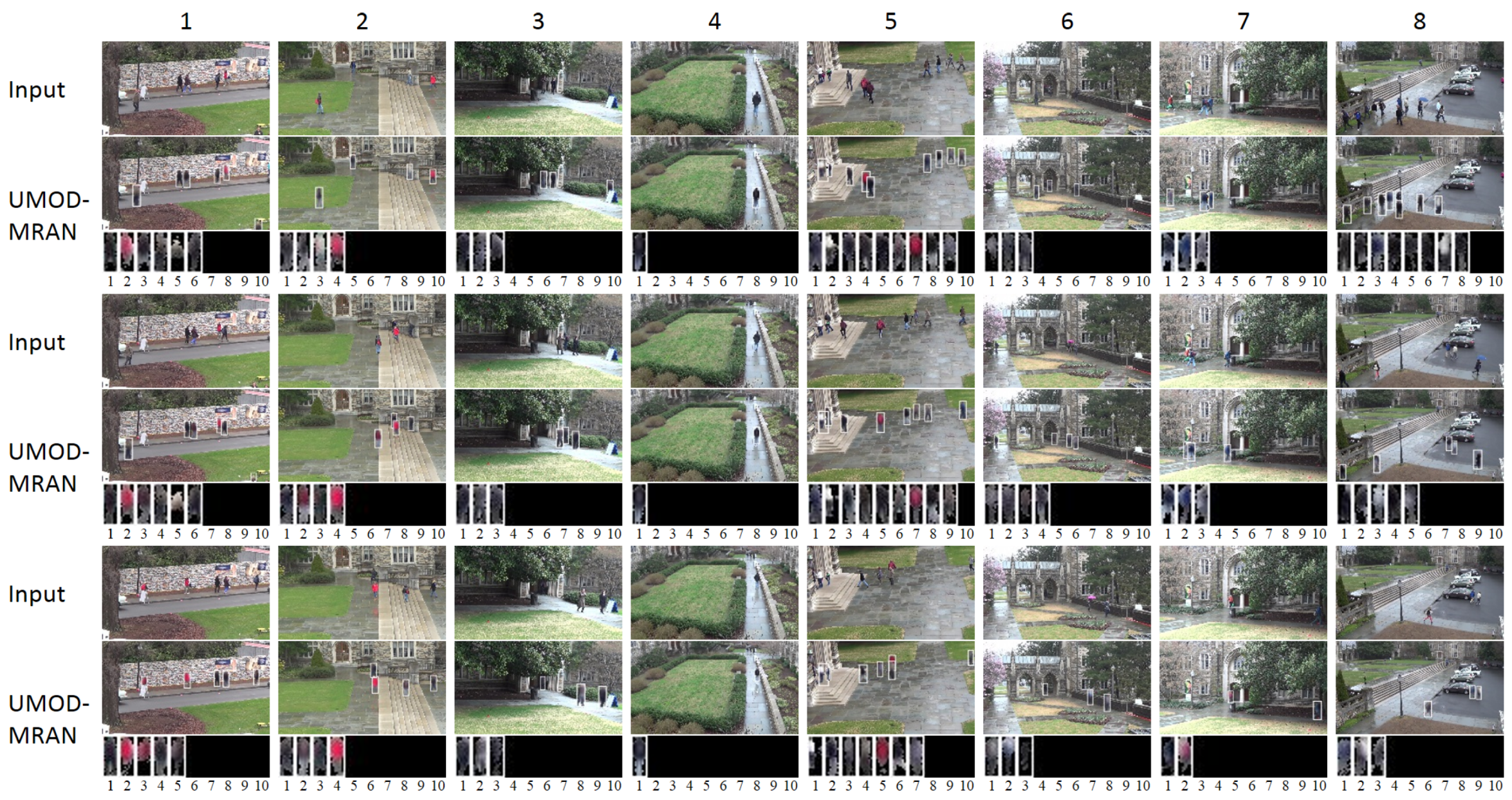
4.2. DukeMTMC
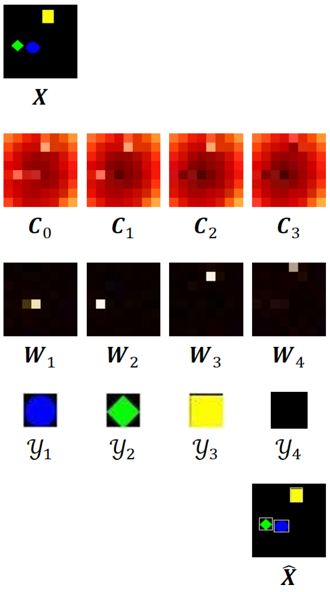
4.3. Visualizing the UMOD-MRAN
5. Related Work
6. Conclusions
Author Contributions
Funding
Conflicts of Interest
References
- Felzenszwalb, P.F.; Girshick, R.B.; McAllester, D.; Ramanan, D. Object detection with discriminatively trained part-based models. IEEE Trans. Pattern Anal. Mach. Intell. 2010, 32, 1627–1645. [Google Scholar] [CrossRef] [PubMed]
- Cortes, C.; Vapnik, V. Support-vector networks. Mach. Learn. 1995, 20, 273–297. [Google Scholar] [CrossRef] [Green Version]
- Girshick, R.; Donahue, J.; Darrell, T.; Malik, J. Rich feature hierarchies for accurate object detection and semantic segmentation. In Proceedings of the IEEE Conference on Computer Vision and Pattern Recognition, Columbus, OH, USA, 23–28 June 2014; pp. 580–587. [Google Scholar]
- Girshick, R. Fast r-cnn. In Proceedings of the IEEE International Conference on Computer Vision, Washington, DC, USA, 7–13 December 2015; pp. 1440–1448. [Google Scholar]
- Ren, S.; He, K.; Girshick, R.; Sun, J. Faster r-cnn: Towards real-time object detection with region proposal networks. In Proceedings of the Advances in neural information processing systems, Montreal, DC, Canada, 7–12 December 2015; pp. 91–99. [Google Scholar]
- He, K.; Gkioxari, G.; Dollár, P.; Girshick, R. Mask r-cnn. In Proceedings of the 2017 IEEE International Conference on Computer Vision (ICCV), Venice, Italy, 22–29 October 2017; pp. 2980–2988. [Google Scholar]
- Enzweiler, M.; Gavrila, D.M. Monocular pedestrian detection: Survey and experiments. IEEE Trans. Pattern Anal. Mach. Intell. 2009, 31, 2179–2195. [Google Scholar] [CrossRef] [PubMed]
- Deng, J.; Dong, W.; Socher, R.; Li, L.J.; Li, K.; Li, F.-F. Imagenet: A large-scale hierarchical image database. In Proceedings of the 2009 IEEE Conference on Computer Vision and Pattern Recognition, Miami, FL, USA, 20–25 June 2009. [Google Scholar]
- Everingham, M.; Van Gool, L.; Williams, C.K.; Winn, J.; Zisserman, A. The pascal visual object classes (voc) challenge. Int. J. Comput. Vis. 2010, 88, 303–338. [Google Scholar] [CrossRef]
- Geiger, A.; Lenz, P.; Stiller, C.; Urtasun, R. Vision meets robotics: The KITTI dataset. Int. J. Robot. Res. 2013, 32, 1231–1237. [Google Scholar] [CrossRef] [Green Version]
- Lin, T.Y.; Maire, M.; Belongie, S.; Hays, J.; Perona, P.; Ramanan, D.; Dollár, P.; Zitnick, C.L. Microsoft coco: Common objects in context. In European Conference on Computer Vision; Springer: Cham, Switzerland, 2014; pp. 740–755. [Google Scholar]
- LeCun, Y.; Boser, B.; Denker, J.S.; Henderson, D.; Howard, R.E.; Hubbard, W.; Jackel, L.D. Backpropagation applied to handwritten zip code recognition. Neural Comput. 1989, 1, 541–551. [Google Scholar] [CrossRef]
- LeCun, Y.; Bottou, L.; Bengio, Y.; Haffner, P. Gradient-based learning applied to document recognition. Proc. IEEE 1998, 86, 2278–2324. [Google Scholar] [CrossRef] [Green Version]
- Huang, L.; Yang, Y.; Deng, Y.; Yu, Y. Densebox: Unifying landmark localization with end to end object detection. arXiv, 2015; arXiv:1509.04874. [Google Scholar]
- Redmon, J.; Divvala, S.; Girshick, R.; Farhadi, A. You only look once: Unified, real-time object detection. In Proceedings of the IEEE Conference on Computer Vision and Pattern Recognition, Las Vegas, NV, USA, 27–30 June 2016; pp. 779–788. [Google Scholar]
- Liu, W.; Anguelov, D.; Erhan, D.; Szegedy, C.; Reed, S.; Fu, C.Y.; Berg, A.C. Ssd: Single shot multibox detector. In European Conference on Computer Vision; Springer: Cham, Switzerland, 2016; pp. 21–37. [Google Scholar]
- Ristani, E.; Solera, F.; Zou, R.; Cucchiara, R.; Tomasi, C. Performance measures and a data set for multi-target, multi-camera tracking. In European Conference on Computer Vision; Springer: Cham, Switzerland, 2016; pp. 17–35. [Google Scholar]
- Rumelhart, D.E.; Hinton, G.E.; Williams, R.J. Learning representations by back-propagating errors. Nature 1986, 323, 533–536. [Google Scholar] [CrossRef]
- Gers, F.A.; Schmidhuber, J.; Cummins, F. Learning to forget: Continual prediction with LSTM. Neural Comput. 2000, 12, 2451–2471. [Google Scholar] [CrossRef] [PubMed]
- Cho, K.; Van Merriënboer, B.; Gulcehre, C.; Bahdanau, D.; Bougares, F.; Schwenk, H.; Bengio, Y. Learning phrase representations using RNN encoder-decoder for statistical machine translation. arXiv, 2014; arXiv:1406.1078. [Google Scholar]
- Jang, E.; Gu, S.; Poole, B. Categorical Reparameterization with Gumbel-Softmax. arXiv, 2016; arXiv:1611.01144. [Google Scholar]
- Jaderberg, M.; Simonyan, K.; Zisserman, A. Spatial transformer networks. In Proceedings of the Advances in Neural Information Processing Systems, Montreal, QC, Canada, 7–12 December 2015; pp. 2017–2025. [Google Scholar]
- Long, J.; Shelhamer, E.; Darrell, T. Fully convolutional networks for semantic segmentation. In Proceedings of the IEEE Conference on Computer Vision and Pattern Recognition, Boston, MA, USA, 7–12 June 2015; pp. 3431–3440. [Google Scholar]
- Graves, A.; Wayne, G.; Danihelka, I. Neural turing machines. arXiv, 2014; arXiv:1410.5401. [Google Scholar]
- Graves, A.; Wayne, G.; Reynolds, M.; Harley, T.; Danihelka, I.; Grabska-Barwińska, A.; Colmenarejo, S.G.; Grefenstette, E.; Ramalho, T.; Agapiou, J.; et al. Hybrid computing using a neural network with dynamic external memory. Nature 2016, 538, 471–476. [Google Scholar] [CrossRef] [PubMed]
- Eslami, S.A.; Heess, N.; Weber, T.; Tassa, Y.; Szepesvari, D.; Hinton, G.E. Attend, infer, repeat: Fast scene understanding with generative models. In Proceedings of the Advances in Neural Information Processing Systems, Barcelona, Spain, 5–10 December 2016; pp. 3225–3233. [Google Scholar]
- Kingma, D.; Ba, J. Adam: A method for stochastic optimization. arXiv, 2014; arXiv:1412.6980. [Google Scholar]
- Stiefelhagen, R.; Bernardin, K.; Bowers, R.; Garofolo, J.; Mostefa, D.; Soundararajan, P. The CLEAR 2006 evaluation. In International Evaluation Workshop on Classification of Events, Activities and Relationships; Springer: Berlin/Heidelberg, Germany, 2006; pp. 1–44. [Google Scholar]
- Bloisi, D.; Iocchi, L. Independent multimodal background subtraction. In CompIMAGE; CRC Press: Boca Raton, FL, USA, 2012. [Google Scholar]
- Yang, B.; Yan, J.; Lei, Z.; Li, S.Z. Craft objects from images. In Proceedings of the IEEE Conference on Computer Vision and Pattern Recognition, Las Vegas, NV, USA, 27–30 June 2016; pp. 6043–6051. [Google Scholar]
- Ren, J.; Chen, X.; Liu, J.; Sun, W.; Pang, J.; Yan, Q.; Tai, Y.-W.; Xu, L. Accurate single stage detector using recurrent rolling convolution. In Proceedings of the IEEE Conference on Computer Vision and Pattern Recognition, Honolulu, HI, USA, 21–26 July 2017. [Google Scholar]
- Kulkarni, T.D.; Whitney, W.F.; Kohli, P.; Tenenbaum, J. Deep convolutional inverse graphics network. In Proceedings of the Advances in Neural Information Processing Systems, Montreal, QC, Canada, 7–12 December 2015; pp. 2539–2547. [Google Scholar]
- Chen, X.; Duan, Y.; Houthooft, R.; Schulman, J.; Sutskever, I.; Abbeel, P. Infogan: Interpretable representation learning by information maximizing generative adversarial nets. In Proceedings of the Advances in Neural Information Processing Systems, Barcelona, Spain, 5–10 December 2016; pp. 2172–2180. [Google Scholar]
- Rolfe, J.T. Discrete variational autoencoders. arXiv, 2016; arXiv:1609.02200. [Google Scholar]
- Le Roux, N.; Heess, N.; Shotton, J.; Winn, J. Learning a generative model of images by factoring appearance and shape. Neural Comput. 2011, 23, 593–650. [Google Scholar] [CrossRef] [PubMed]
- Moreno, P.; Williams, C.K.; Nash, C.; Kohli, P. Overcoming occlusion with inverse graphics. In Proceedings of the Advances in Neural Information Processing Systems, Barcelona, Spain, 5–10 December 2016; pp. 170–185. [Google Scholar]
- Huang, J.; Murphy, K. Efficient inference in occlusion-aware generative models of images. arXiv, 2015; arXiv:1511.06362. [Google Scholar]
- Yan, X.; Yang, J.; Yumer, E.; Guo, Y.; Lee, H. Perspective transformer nets: Learning single-view 3d object reconstruction without 3D supervision. In Proceedings of the Advances in Neural Information Processing Systems, Barcelona, Spain, 5–10 December 2016; pp. 1696–1704. [Google Scholar]
- Rezende, D.J.; Eslami, S.A.; Mohamed, S.; Battaglia, P.; Jaderberg, M.; Heess, N. Unsupervised learning of 3D structure from images. In Proceedings of the Advances in Neural Information Processing Systems, Barcelona, Spain, 5–10 December 2016; pp. 4996–5004. [Google Scholar]
- Stewart, R.; Ermon, S. Label-free supervision of neural networks with physics and domain knowledge. In Proceedings of the Thirty-First AAAI Conference on Artificial Intelligence, San Francisco, CA, USA, 4–9 February 2017. [Google Scholar]
- Wu, J.; Tenenbaum, J.B.; Kohli, P. Neural scene de-rendering. In Proceedings of the Computer Vision Foundation, Honolulu, HI, USA, 21–26 July 2017. [Google Scholar]
- Graves, A. Adaptive computation time for recurrent neural networks. arXiv, 2016; arXiv:1603.08983. [Google Scholar]


| Hyper-parameter | Sprites | DukeMTMC | ||
|---|---|---|---|---|
| [128, 128, 3] | [108, 192, 3] | |||
| (FCN) | Kernel size | Layer size | Kernel size | Layer size |
| [5, 5] | [64, 64, 32] | [5, 5] | [108, 192, 32] | |
| [3, 3] | [32, 32, 64] | [5, 3] | [36, 64, 128] | |
| [1, 1] | [16, 16, 128] | [5, 3] | [18, 32, 256] | |
| [3, 3] | [8, 8, 256] | [3, 1] | [9, 16, 512] | |
| [1, 1] | [8, 8, 20] | [1, 1] | [9, 16, 200] | |
| [8, 8, 20] | [9, 16, 200] | |||
| R | 40 | 400 | ||
| (FC) | 40 → 266 → 1772 | 400 → 578 → 836 | ||
| [21, 21, 3] | [9, 23, 3] | |||
| Configuration | AP↑ | MODA↑ | MODP↑ | FAF↓ | TP↑ | FP↓ | FN↓ | Precision↑ | Recall↑ |
|---|---|---|---|---|---|---|---|---|---|
| UMOD-MRAN | 96.8 | 95.3 | 91.5 | 0.02 | 21,016 | 234 | 807 | 98.9 | 96.3 |
| UMOD-MRAN-noOcc | 92.7 | 90.3 | 90.3 | 0.04 | 20,121 | 415 | 1702 | 98.1 | 92.2 |
| UMOD-RNN | 94.5 | 94.1 | 90.6 | 0.03 | 20,819 | 284 | 1004 | 98.7 | 95.4 |
| AIR | 90.5 | 88.2 | 88.6 | 0.06 | 19,859 | 611 | 1964 | 97.2 | 91.0 |
| Method | AP↑ | MODA↑ | MODP↑ | FAF↓ | TP↑ | FP↓ | FN↓ | Precision↑ | Recall↑ |
|---|---|---|---|---|---|---|---|---|---|
| DPM [1] | 79.3 | 66.9 | 83.4 | 0.32 | 108,050 | 22,445 | 19,820 | 82.8 | 84.5 |
| Faster R-CNN [5] | 89.7 | 82.1 | 87.5 | 0.13 | 114,443 | 9,413 | 13,427 | 92.4 | 89.5 |
| CRAFT [30] | 91.1 | 83.4 | 89.8 | 0.12 | 115,850 | 8,586 | 12,020 | 93.1 | 90.6 |
| RRC [31] | 92.0 | 84.3 | 90.7 | 0.13 | 116,873 | 9,068 | 10,997 | 92.8 | 91.4 |
| UMOD-MRAN (ours) | 87.2 | 78.7 | 85.3 | 0.15 | 111,247 | 10,601 | 16,623 | 91.3 | 87.0 |
© 2018 by the authors. Licensee MDPI, Basel, Switzerland. This article is an open access article distributed under the terms and conditions of the Creative Commons Attribution (CC BY) license (http://creativecommons.org/licenses/by/4.0/).
Share and Cite
He, Z.; He, H. Unsupervised Multi-Object Detection for Video Surveillance Using Memory-Based Recurrent Attention Networks. Symmetry 2018, 10, 375. https://doi.org/10.3390/sym10090375
He Z, He H. Unsupervised Multi-Object Detection for Video Surveillance Using Memory-Based Recurrent Attention Networks. Symmetry. 2018; 10(9):375. https://doi.org/10.3390/sym10090375
Chicago/Turabian StyleHe, Zhen, and Hangen He. 2018. "Unsupervised Multi-Object Detection for Video Surveillance Using Memory-Based Recurrent Attention Networks" Symmetry 10, no. 9: 375. https://doi.org/10.3390/sym10090375
APA StyleHe, Z., & He, H. (2018). Unsupervised Multi-Object Detection for Video Surveillance Using Memory-Based Recurrent Attention Networks. Symmetry, 10(9), 375. https://doi.org/10.3390/sym10090375