A Coarse-to-Fine Approach for 3D Facial Landmarking by Using Deep Feature Fusion

Abstract

Facial landmarking locates the key facial feature points on facial data, which provides not only information on semantic facial structures, but also prior knowledge for other kinds of facial analysis. However, most of the existing works still focus on the 2D facial image which may suffer from lighting condition variations. In order to address this limitation, this paper presents a coarse-to-fine approach to accurately and automatically locate the facial landmarks by using deep feature fusion on 3D facial geometry data. Specifically, the 3D data is converted to 2D attribute maps firstly. Then, the global estimation network is trained to predict facial landmarks roughly by feeding the fused CNN (Convolutional Neural Network) features extracted from facial attribute maps. After that, input the local fused CNN features extracted from the local patch around each landmark estimated previously, and other local models are trained separately to refine the locations. Tested on the Bosphorus and BU-3DFE datasets, the experimental results demonstrated effectiveness and accuracy of the proposed method for locating facial landmarks. Compared with existed methods, our results have achieved state-of-the-art performance.

1. Introduction

Accurate and automatic facial landmark detection or face alignment is critical in face verification, face recognition, facial animation, facial expression recognition and other research. Therefore, it attracts increasing research interests worldwide.

Recently, most studies on face alignment are still primarily conducted on texture images [1,2,3,4,5,6,7,8,9,10]. As known, 2D face images are rather sensitive to some condition changes such as arbitrary pose and illumination variations. To address the pose limitation, some researchers proposed that using the reconstructed 3D shape can assist facial landmarking performance under arbitrary poses [11,12]. However, the reconstructed 3D face shape based on corresponding 2D face texture is still sensitive to illumination changes. Motivated by this challenge, the emergence of 3D facial data has provided an alternative to enhance the accuracy and efficiency of facial landmarks’ estimation.

With the progress of 3D technology, locating facial landmarks on the 3D facial data has been widely studied [13,14,15,16,17,18,19,20,21]. Unlike 2D images, both facial geometry information and texture information is contained in each piece of 3D facial data. During the past decade, more studies about facial landmarks’ estimation on 3D facial data have been presented. Most of the approaches [20,21,22] applied both texture data and geometry data to detect landmarks jointly, which can enhance the performance effectively. In fact, not all 3D scanners provide texture and the texture information is not invariant to viewpoint and lighting conditions, so it is necessary to locate landmarks accurately only from 3D geometry data. However, most studies only take range data into account and don’t make the best of features extracted from 3D geometry data. In contrast, Li [23] employs feature fusion to recognize facial expression and make great progress. Motivated by this, our proposed method would take five facial attribute maps extracted from 3D geometry data, instead of only applying the range data.

In this paper, we proposed a general framework based on coarse-to-fine for face landmarking only taking 3D facial geometry data. As Figure 1 illustrates, we firstly proposed five feature maps computed from pre-processed 3D geometry data, including a range map, three surface normal maps and a curvature map, which are insensitive to lighting conditions. To locate landmarks accurately, a cascade regression network was designed to update landmarks location iteratively. For this purpose, the global CNN feature extracted by a pre-trained deep neural network from five feature maps was used to estimate landmarks roughly. According to learning the mapping functions from the fused local CNN feature around the landmark estimated previously to corresponding residual distance, local refinement nets are trained independently. By adopting the coarse-to-fine strategy, the performance of landmarking would be improved iteratively.

In summary, our learning-based framework is a novel coarse-to-fine approach to estimate landmarks on 3D geometry data by fusing the deep CNN features. The main contributions of this work are the following:

• We propose using the deep CNN feature extracted from five kinds of facial attribute maps to estimate 3D landmarks jointly, instead of using any handcrafted features.
• We propose a global estimation stage and a local refinement stage for 3D landmarks’ prediction based on coarse-to-fine strategy and feature fusion.
• Tested in the public 3D face datasets named Bosphrous and BU-3DFE databases, the performances have been state-of-the-art.

The rest of this paper is organized as follows: Section 2 briefly reviews related works about 2D and 3D landmarks’ localization. Section 3 describes our proposed method in detail. In this section, the architecture of proposed model, global estimation and local refinement will be introduced. Experimental results are evaluated and compared in Section 4. The weakness of the proposed approach will be discussed in Section 5. Section 6 includes the conclusions and future research derived from this work.

2. Related Work

2.1. Facial Landmarking on 2D Images

Various 3D based methods are the extension of 2D-based. The 2D facial landmarking can generally be divided into two main categories: model-based [1,2,3] and regression-based [4,6,7] methods. In the former category, it mainly builds face templates to fit the input images, such as Active Appearance Model (AAM) [1], Active Shape Model (ASM) [2], and Constrained Local Model (CLM) [3]. However, model-based methods do not perform not very well in the wild, mainly because the linear model can’t handle the complex nonlinear model well. Thus, the regression-based method was proposed to estimate landmark locations explicitly by regression models. It also has been the most widely employed and has made great progress. Supervised Descent Regression (SDR) [6], Cascade Fern Regression (CFR) [7], and Random Forest Regression (RFR) [4] have been established to deal with face alignment on 2D face images. However, most regression-based methods [5,8,9,10] refine an initial landmark location iteratively, and the performance under some challenging conditions such as illumination changes are not very satisfactory.

Recently, research on deep learning has become a popular field of study with the development of computer hardware and the theory of neural networks. Face recognition [24,25], face verification [26] and facial expression recognition [27] have achieved better performance than the traditional approaches. Compared with the traditional methods, deep learning-based methods have been emerging as an innovative branch in facial landmarking studies recently. Cascade CNN [28], coarse-to-fine Auto-encoder Networks (CFAN) [29] and deep multi-task [30] learning methods are proposed to locate landmarks accurately. Stacked hourglass networks [31] are proposed to estimate landmarks end-to-end. In essence, deep-learning based methods are still regression-based methods which adopt deeper neural networks to estimate the nonlinear correlation between facial image and estimated landmarks. However, it is a great challenge to acquire a huge amount of face data and corresponding labels. Some methods are built on three-dimensional assistance. In Zhu [11], Jourabloo [12] and Kumar [32], they all adopt a 3D solution in a novel alignment framework, which shows that the character of 3D data can help to conquer the limitation of arbitrary pose and other challenges. In Bulat [33], they created a large dataset and estimated 2D and 3D landmarks by adopting hourglass networks. However, all of these methods obtain corresponding 3D shape by adopting 3DMM or 2D texture images that is also sensitive to the changeable lighting conditions.

2.2. Facial Landmarking on 3D Facial Data

Many studies on face landmarking based on 3D geometry and texture data jointly have been proposed recently.

In most of the existing works on 3D facial landmarking, 3D facial landmarks are estimated by computing the 3D shape-related feature, including shape index [14,15,34], effective energy [16], Gabor filter [17,18], local gradient [35] and curvature feature [36]. However, the accuracy on these prominent landmarks decreases drastically, including nose tip and the corner of eyes.

Among these methods on 3D facial landmarking, many approaches utilize registered range data and texture images jointly to estimate landmarks straightforwardly, which can take full advantage of the information from range and texture data. In Boehnen and Russ [37], the eye and mouth maps are computed by adopting both range and texture information. In Wang et al. [38], a point signature representation and the Gabor jets from 2D texture images are used to represent the 3D face mesh. Salah and Jahanbin et al. [22,39] proposed the Gabor wavelet coefficient so that the local appearance in 2D texture image and local patch in the range data around each landmark can be modeled well. As the same thought, in Lu and Jain [40], the local shape index feature and cornerness texture feature around seven landmarks were computed and fused to detect landmarks jointly.

Unlike the above approaches which estimate each landmark independently, the combination of candidate landmarks is quite essential to improve the performance. To make use of the structure between each landmark, the heuristic model [21], 3D geometry-based model [37] and elastic bunch graph-based model [22] were proposed. Most of the works constructed the average 3D position of landmarks as the initialization shape and then updated the position iteratively. However, all of these approaches didn’t consider the relationship between the 3D position of landmarks and the feature around each landmark, including the range feature and texture feature. In addition, the 3D point distribution model (PDM) was proposed to estimate eyes, nose and mouth corner. Nair and Cavallaro [21] study 3D facial landmarking by building a statistical model to estimate landmarks coarsely, and then heuristics are applied to refine the locations. Perakis et al. [14,15] study landmarking on 3D facial data under much more challenging conditions, such as the missing data caused by self occlusion. Zhao et al. [20] proposed another method based on statistical models, who presented a model which take the both the relationship between each landmark and the local properties around each landmark into account. However, the main problem of this approach is that the solution is not global, which was caused by the inappropriate initialization.

3. Methodology

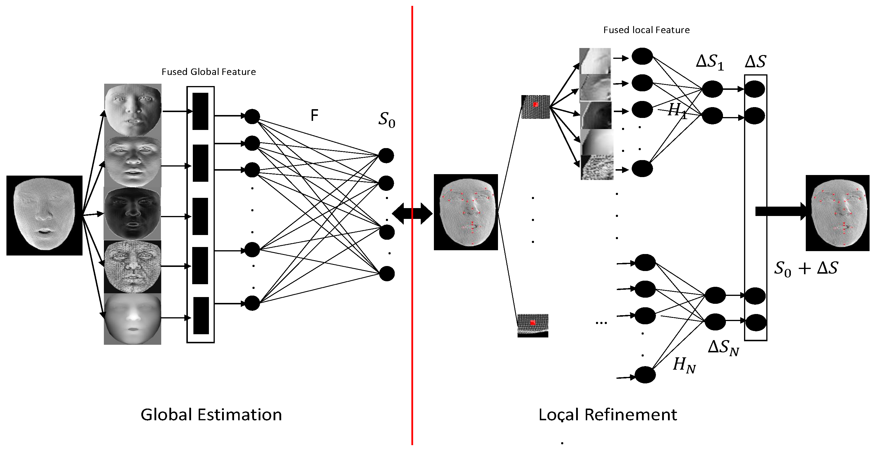
3.1. Overview

Given a 3D facial geometry data G, 3D facial landmarks’ detection is the task to locate N pre-defined fiducial points, including eye corners, nose tip, mouth corners and so on. We denote the homogeneous coordinate of 3D facial landmarks as S:

$$\begin{array}{c}\hfill S=\left(\begin{array}{cccc}{x}_1& x_2& \dots & x_N\\ y_1& y_2& \dots & y_N\\ z_1& z_2& \dots & z_N\end{array}\right),\end{array}$$

(1)

where N is the pre-defined number of landmarks. The function is also equal to the following function:

$$\begin{array}{c}\hfill S=\left(\begin{array}{cccc}x(u_1,v_1),& x(u_2,v_2),& \dots & x(u_N,v_N)\\ y(u_1,v_1),& y(u_2,v_2),& \dots & y(u_N,v_N)\\ z(u_1,v_1),& z(u_2,v_2),& \dots & z(u_N,v_N)\end{array}\right),\end{array}$$

(2)

where x,y and z represent the x,y,z coordinate map for each pair $(u,v)$. Given 3D facial data, our goal is to simultaneously estimate the $(u,v)$ accurately.

For this purpose, we propose transforming the 3D face landmarks’ estimation to detect the landmarks on five types of 2D facial attribute maps, including shape index map, normal maps and original range map that calculated on 3D geometry data. Then, a novel framework as Figure 1 was presented to achieve our goal accurately and efficiently. Based on the coarse-to-fine strategy, the framework comprises two main parts: one is for global estimation and the other is for local refinement. Specifically, the global estimation phase is intended to locate the landmarks roughly by feeding into the fused global feature that extracted from these attribute maps. Then, the local refinement stage is to learn the nonlinear mapping function from the fused local feature that extracted from a local patch around estimated global landmarks to residual distance.

In the global estimation phase, the goal is to locate landmarks roughly, but it is still more robust and accurate than the mean shape. To train this model, instead of applying the handcrafted feature, we use the pre-trained deep network to extract features from each facial attribute map as a global feature and then concatenate them as the fused feature. Feeding into the fused feature, the target of the regression model is to estimate global landmarks directly. According to the trained model, the global landmarks would be obtained roughly but robustly, which can lay the foundation for the local refinement.

After global optimization by inputting the fused global feature, we can get the initialization shape. The initialization shape is more robust and accurate than the mean shape; however, it is still not satisfied. To refine the global estimation, the refinement stage is designed to refine the results. We extract the local CNN feature from the cropped local patches around the global landmarks and then learn the mapping function from the fused local feature to the residual distance between previous landmarks and ground truth.

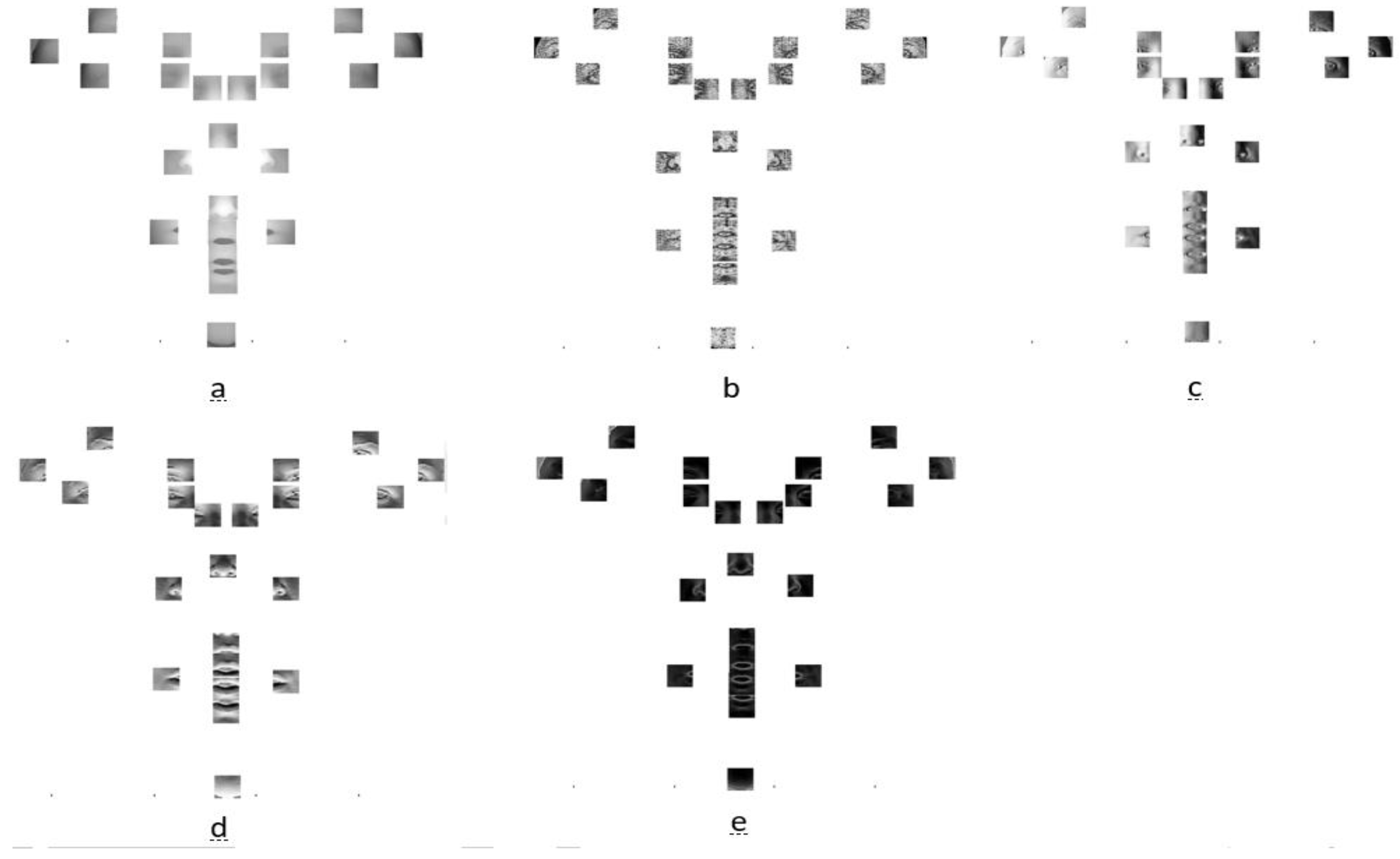
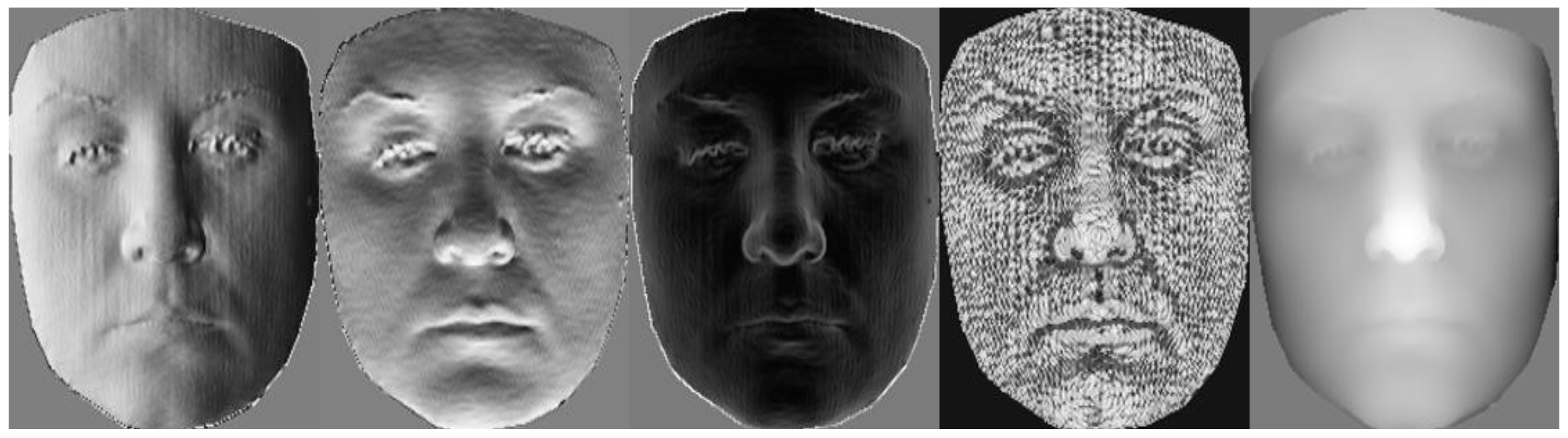
3.2. Facial Attribute Maps

To comprehensively describe the geometric information of 3D data, five types of facial attribute maps were constructed, including three surface normal maps $Nx$, $Ny$, $Nz$, curvature feature $SI$, and range data R. Among these maps, surface curvature and normal maps are the most significant feature in 3D object detection, recognition and other 3D tasks. Figure 2 shows the five types of facial attribute maps computed from original 3D facial geometry data.

3.2.1. Surface Curvature Feature

The surface curvature features have been adopted for 3D face landmarks’ estimation in many types of research. Actually, surface curvature is the most significant feature in 3D object detection, recognition and other 3D tasks. Thus, this paper chooses the shape index feature map as the first facial attribute.

The Shape index is a continuous mapping of principal curvature values $\left(k_{max},k_{min}\right)$ of a 3D object point p. Once we have two principal curvature $\left(k_{max},k_{min}\right)$, the shape index values, which describe different shapes classed as single numbers ranging from 0 to 1, are calculated as:

$$SI\left(p\right)=\frac{1}{2}-\frac{1}{\pi }arctan\left(\frac{k_{max}+k_{min}}{k_{max}-k_{min}}\right).$$

(3)

3.2.2. Surface Normal Maps

Considering a normalized 3D facial geometry data G, denoted as a $m\times n\times 3$ matrix:

$$G={\left[P_{uv}(x,y,z)\right]}_{m\times n}={[p_{uvx},p_{uvy},p_{uvz}]}_{1\le u\le m,1\le v\le n},$$

(4)

where $\left[P_{uv}(x,y,z)\right]$ denotes the corresponding 3D point coordinate of facial geometry data. The corresponding surface normal maps are represented as:

$$\begin{array}{c}\hfill N\left(I_g\right)=N{\left[P_{uv}(x,y,z)\right]}_{m\times n}\\ \hfill ={[N\left(p_{uvx}\right),N\left(p_{uvy}\right),N\left(p_{uvz}\right)]}_{1\le u\le m,1\le v\le n}.\end{array}$$

(5)

In this paper, a local plane fitting method is applied to compute $N\left(I_g\right)$, which consists of a three $M\times n$ matrix. In other words, for each point in 3D facial geometry data, the surface normal vector can be computed by the following function:

$$S_{uv}:N_{uvx}{q}_{uvx}+N_{uvy}{q}_{uvy}+N_{uvz}{q}_{uvz}=d,$$

(6)

where $(q_{uvx},q_{uvy},q_{uvz})$ represents any point within the local neighbourhood of point $p_{uv}$ and ${∥{\left(N_{uvx},N_{uvy},N_{uvz}\right)}^T∥}_2=1$. In this paper, a neighbourhood of $5\times 5$ window is adopted and three normal maps would be obtained, denoted as $N_x,N_y,N_Z$.

3.3. Global Estimation

As the proposed method illustrates, these five types of attribute maps as Figure 2 would be fed into the neural network to estimate landmarks roughly. Considered the calculated feature maps, denoted as shape index $SI$, $N_x$, $N_y$, $N_z$ and original range map R, $S_g\left(x\right)\in R^{2N\times 1}$ represents the ground truth of N landmarks. The goal of our global model is to learn the mapping function F from our fused feature map to the ground truth coordinate:

$$\begin{array}{c}\hfill S_g\left(x\right)\leftarrow F\left(SI,N_x,N_y,N_z,R\right).\end{array}$$

(7)

Limited to the amount of training data, training a global CNN model directly is always over-fitting. To overcome this limitation, fine-tuning based on a pre-trained deep model was employed to learn F. To achieve this goal, the parameters of pre-trained model were fixed except training the last layer. Then, the $SI$, $N_x$, $N_y$, $N_z$, R are fed into the pre-trained model (e.g., VGG (Visual Geometry Group)-net in this paper) separately. Generally, the pre-trained deep CNN model can be regarded as a special feature extractor, which can be regarded as $v=DNN\left(Map\right)$, where $DNN$ represents the fixed part of the pre-trained model, $Map$ denotes the resized facial attribute map, and v is the extracted feature vector of each attribute map. Consider adopting shape index maps and convolution neural networks to detect a coarse $S_0$ as the result of the first step. In particular, the deep models are all comprised of three main parts including convolutional layers, pooling layers and fully connected layers.

• Convolutional Layer and ReLU Non-linearity.

Through a set of designed and learnable filters, the convolutional layer transforms the input images or activation maps to another. Specifically, given a set of activation maps from the previous layer $y^{l-1}\in {\mathbb{R}}^{W_{l-1}\times H_{l-1}\times D_{l-1}}$, and $K_l$ convolutional filters, each with size $W_f\times H_f\times D_{l-1}$, a list of activation maps $y^l\in {\mathbb{R}}^{W_l\times H_l\times D_l}$ at the layer L will be computed and output. Let this stride be S; then, the $W_l=(W_{l-1}-W_f+2P)/S+1$ and $H_l=(H_{l-1}-H_f+2P)/S+1$. Then, we add an activation function $\phi$ to adjust the result to a nonlinear function. In this paper, rectified linear units (ReLU), denoted as $\phi \left(x\right)=max\left(0,x\right),$ is used. Thus, the result of l layer is denoted as:

$$y^l=\phi (W_l\ast y^{l-1}+b_l),$$

(8)

where $b_l$ denotes the bias term, and ∗ denotes the convolution operator.

• Fully Connected layers.

This layer is used to reshape these feature maps into a vector feature. The hidden layers are fully connected, which means that each unit in a previous layer is connected with each unit in the next layer. Suppose the global network has L convolutional layers in total and so the feature maps in the last convolutional layers are represented as $y^l\in {\mathbb{R}}^{W_L\times H_L\times D_L}$. Let the $(L+1)$-th layer be the fully connected layer, and the output of layer L be the input of layer $L+1$, with size $y^{L+1}\in {\mathbb{R}}^K,$ where $K=W_L\times H_L\times D_L$. Thus, this layer is equal to:

$$y^{L+1}=reshape\left(y^L\right).$$

(9)

Then, the next fully connected layer will be:

$$y^{L+2}=\phi (w^{L+1}\times y^{L+1}+b^{L+1}),$$

(10)

where $W^{L+1}$ is the weight value in the $L+1$-th layer and $b^{L+1}$ is the bias term value. $\phi$ denotes the tanh activation function. C. Objective function. After feature extraction for each facial attribute map is done separately, the feature vectors are concatenated as $V=\left[v_{SI},v_{N_x},v_{N_y},v_{N_z},v_R\right]$ to train the global model F. Specifically, by training a designed neural networks, our target has been formulated as solving the objective function:

$$\begin{array}{c}\hfill argmin{∥S_g-F\left(V\right)∥}_2^2,\end{array}$$

(11)

where F is the nonlinear regression function from V to the landmarks $S_g$, denoted as $F=\sigma \left(W^{T}V+b\right)$, where $\sigma$ represents the nonlinear activation function such as sigmoid, tanh and Relu. In this paper, sigmoid function is employed by the final output layer to learn the parameters $[W,b]$. However, the range of final output is $[0,1]$, while the range of regression is inconsistent. Therefore, $S_g$ would be normalized to range $[0,1]$, so that the objective function can be formulated as minimizing the function:

$$\begin{array}{c}\hfill argmin{∥S_g-F\left(V\right)∥}_2^2+\lambda {∥W∥}_F^2,\end{array}$$

(12)

where ${∥W∥}_F^2$ denotes the regularization term, added to prevent the over-fitting. $\lambda$ is the set to $0.00005$.

After the optimization with Equation (12), the learned parameters $\left[W,b\right]$ are obtained and $S_0$ would be calculated via $S_0=F\left(V\right)$.

3.4. Local Refinement

The global estimation phase describes the mapping function from the fused facial attribute maps to the target landmarks’ location. Unlike other methods, the estimated shape is global and more accurate than the mean shape. However, it is still rough and there is room for improvement. To achieve more accurate locations, a coarse-to-fine based approach is proposed to improve the performance. Similar to many cascade regression methods for 2D face alignment, a local model as Figure 3 is employed to estimate the residual distance $\Delta S$, representing the distance between global estimated shape $S_0$ and ground truth $S_g$.

Similar to the global estimation, we employed the pre-trained CNN model to extract local features from the local patches around the estimated shape $S_0$. Each local patch around $S_0$ is cut out within $30$mm, and then transformed to attribute maps. After the calculation of local attribute maps, they would be resized to $224\times 224$ and are fed into the pre-trained deep neural network to extract local CNN features. Actually, we once considered concatenating the fused local feature of all landmarks to estimate the $\Delta S$ jointly. However, limited to the huge number of trained parameters (e.g., $4096\times 5\times 22\times 44=$ 19,824,640), we propose refining each local patch around a landmark independently. For this purpose, deep feature fusion is also applied for training local model, denoted as ${\varphi }_i={[{\varphi }_{SI}^i,{\varphi }_{Nx}^i,{\varphi }_{Ny}^i,{\varphi }_{Nz}^i,{\varphi }_R^i]}_{i=1,2,\dots N}$, where i represents the i-th landmark and N is the number of located landmarks.

Getting the local feature vectors, the local refinement model is to learn a nonlinearity function $H_i$ from fused local feature ${\varphi }_i$ to the $\Delta S_i$ for each landmark, denoted as $\Delta S_i=S_g\left(i\right)-S_0\left(i\right)$. The objective function of each model can be formulated as follows:

$$\begin{array}{c}\hfill argmin{∥\Delta S_i-H_i\left({\varphi }_i\right)∥}_2^2+\beta {∥W_k∥}_F^2,\end{array}$$

(13)

where $H_i$ is a regression function the same as F, represented as $H_i=\sigma \left(W_i{\varphi }_i+b_i\right)$. Different from the global estimation, the activation function $\sigma$ is the tanh function, so that all the outputs are in range $[-1,1]$. After optimization, we can compute $\Delta S_i$ according to $\Delta S_i=H_i\left({\varphi }_i\right)$, and then we obtain $\Delta S=\left[\Delta S_1,\Delta S_2,\dots \Delta S_N\right]$. Therefore, normalized results $S_{final}$ can be computed as the following:

$$\begin{array}{c}\hfill S_{final}=\Delta S+S_0.\end{array}$$

(14)

4. Experiments

We firstly introduce the datasets used in this paper and then will describe data pre-processing, data augmentation and the parameters’ setting briefly in this section. Finally, we will evaluate the performance in these datasets and compare their performances with other methods.

4.1. Datasets

To evaluate the proposed approach, we employ two public 3D facial data, namely the Bosphorus database [41] and the BU-3DFE (Binghamton University 3D Facial Expression) database [42].

The Bosphorus database contains 4666 pairs facial scans from 105 subjects. It also contains 3D facial geometry data under various occlusions (e.g., glass, hands and hair) and several facial expressions. In our experiments, all of the nearly frontal facial data are selected regardless of the occlusion and expressions, resulting in 3632 3D facial geometry data in total. However, the number of landmarks in these data is inconsistent, so we manually selected and labelled 22 landmarks in the Bosphorus dataset for training the models.

The BU-3DFE database includes data from 100 subjects which contain 56 female and 44 male. Each subject contains not only a neutral expression but also the six universal expressions. In our experiments, we have selected all near frontal facial data from all the subjects, regardless of the expression variance, getting 2500 facial scans totally. In this dataset, among the labelled 83 landmarks, we manually selected 68 landmarks and abandoned the other 15 landmarks located on the facial edge. Actually, some common landmarks are labelled in the two datasets, such as eye corners and mouth corners.

4.2. Data Pre-Processing

To learn the global and local attribute maps, the size of global and local patches needed to be resized to the same size, meaning that the number of 3D clouds for each piece of 3D facial geometry data is uniform. However, it is hard to be normalized because of the different face scales. Therefore, uniform grids are applied to remesh the global facial scans or local regions around landmarks. To get local regions, we select all of the points around the landmark with a specific size of $30\mathrm{mm}\times 30\mathrm{mm}$, and then remesh a uniform grid with the same number of points by using the interpolation. At the same time, the z-values on this grid would be processed by using this normalization. Based on the uniform grids, the facial attribute maps and local patches would be constructed easily and efficiently.

4.3. Data Augmentation

In fact, the number of training data in these datasets is not enough to avoid over-fitting. To overcome over-fitting and improve the performance, increasing the number of training data by utilizing data augmentation is necessary and useful. For this purpose, randomly rotation and symmetry transformation were chosen to augment the variety of facial data. Firstly, we randomly rotate facial data in the horizontal direction and ensure that the face is nearly frontal. Secondly, we also transform the symmetry data for each piece of training data. After data augmentation, more artificially generated facial data would be obtained, so that the over-fitting can be addressed effectively. Of course, the corresponding ground truth would be changed by the same rules.

4.4. Experimental Setting

In our paper, the pre-trained deep CNN model, namely VGG16 [43], is selected for extracting deep CNN features. In the pre-trained networks, all layers and parameters are kept unchanged in the network except the final fully connected layer. As known, the size of the input map is $224\times 224$ and the dimension of features is 4096. Since we have five types of facial, the dimension of fused feature is $4096\times 5$, while the number of output units is $2\times N$. The weight matrix W with size $(4096\times 5)\times (2\times N)$ would be randomly initialized, and corresponding bias vector b would be initialized by a $2\times N$-dimensional zero vector. Each local refinement network is almost similar to the global estimation network, and the number of output units is 2. The weight matrix $W_i$ with size $(4096\times 5)\times 2$ would be also randomly initialized, and the corresponding bias vector $b_i$ would be initialized by a two-dimensional zero vector.

4.5. Convergence and Model Selection

To train these models appropriately, we trained the global estimation model and local refinement models for 2000 iterations, so that these models can converge. Actually, these models have been in convergence when the models were trained about for 1600 iterations. However, to avoid over-fitting in these testing data, the models which trained for about 1400 iterations would be chosen, which may be closed to convergence and more suitable in the testing dataset. The experiments also show that these models perform much better in the testing data.

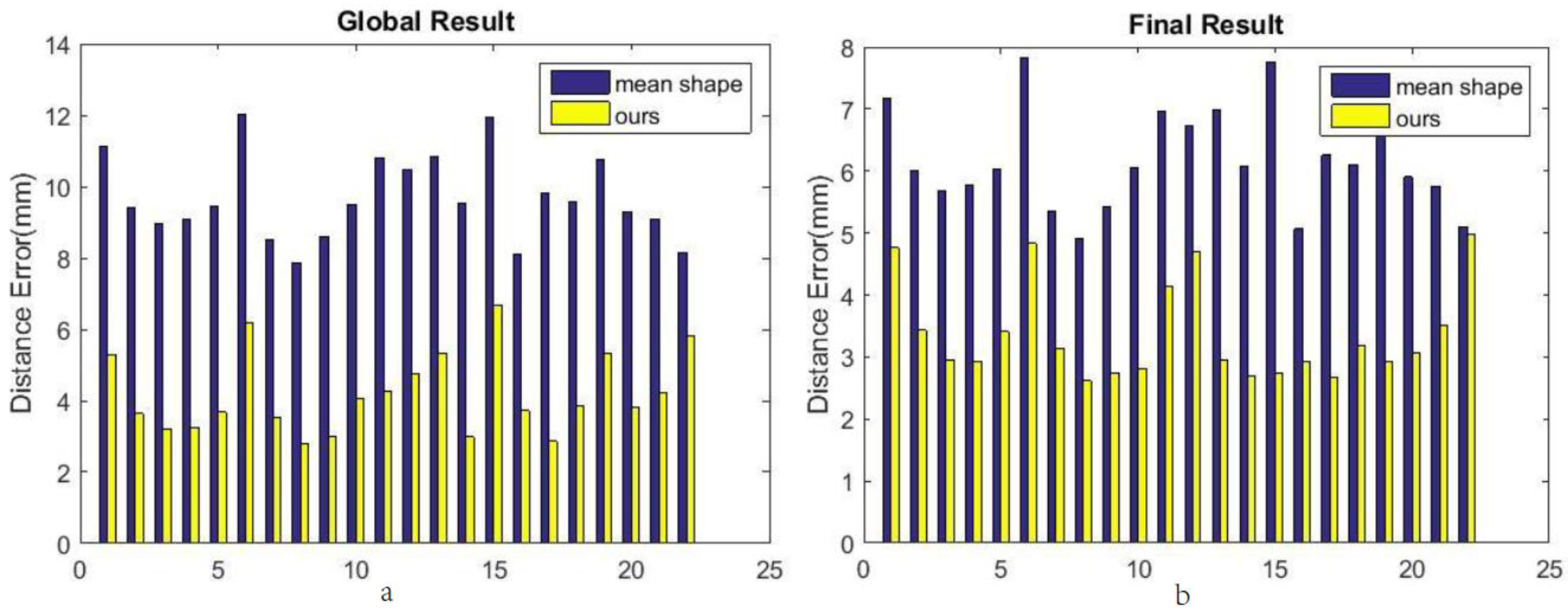
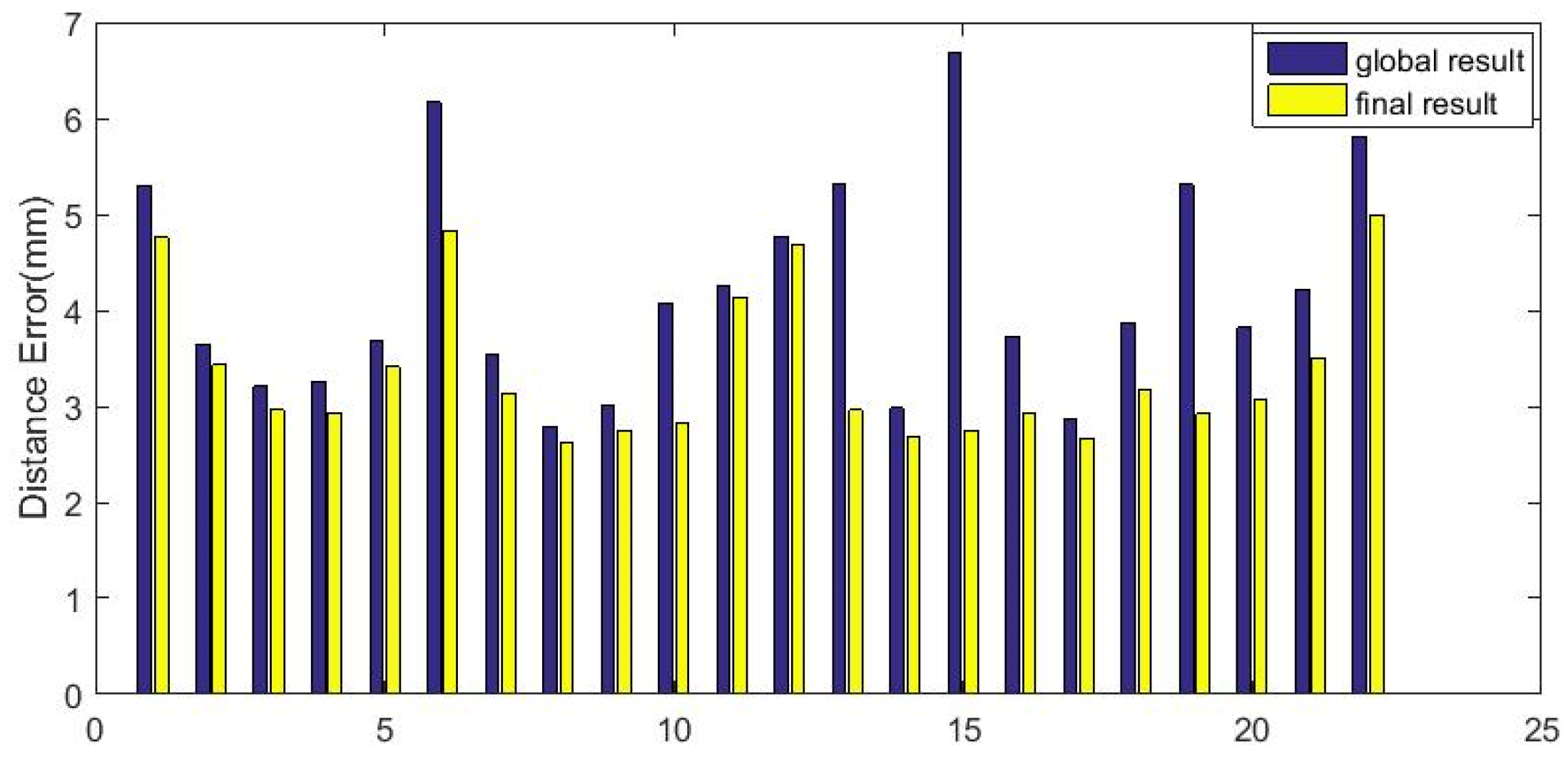
4.6. Evaluation

To evaluate our proposed approach, three comparison experiments are designed in this section. First, it is necessary to confirm the efficiency of coarse-to-fine strategy. Second, the performance by using mean shape as initialization shape is evaluated. Furthermore, the third is to show the performances under different feature combination. In all experiments, distance error calculated as Euclidean distance between estimated landmarks location and corresponding ground truth were used to evaluate the performance. To evaluate and compare these methods, these three main experiments are carried out on the Bosphorus dataset. Among these 3632 data, 2800 data are randomly selected as training data, and the other 832 are regarded as testing data. The number of training data is increased to $2800\times 6=$ 16,800 after augmentation. In this section, all models are trained and tested by using the same training and testing data.

To confirm the effective of global estimation, we compare our method with the method by taking mean shape as initialization shape. Different from taking the global estimation as initialization, mean shape is computed as the initialization shape for local refinement. Instead of global estimation, the local patches around mean shape are taken to extract local features. Then, we will update the locations the same as the local refinement phase in our method. Figure 4a shows the average distance error after global estimation and mean shape calculation, and Figure 4b illustrates the average distance error via two different initialization ways after local refinement. As can be seen, the results of our proposed method outperforms after the local refinement.

Furthermore, to verify the coarse-to-fine strategy, we compare the results after global estimation and local refinement. In Figure 5, the blue bars show the average distance error of 22 landmarks in the testing dataset after global estimation, while the other bars show the results after refinement. It can be easily observed that the results are enhanced effectively from coarse to fine. Note that the mean error has achieved $4.11$mm after global estimation, while $98.23\%$ landmarks are located automatically with $20$mm and $93.31\%$ landmarks are with $10$mm. After local refinement, the $100\%$ landmarks are located automatically with $20$mm precision and $96.43\%$ are with $10$mm. Furthermore, the average error of all landmarks in the testing data can also be improved to $3.37$mm, which has achieved the state-of-the-art.

To show the performance under different feature combinations, the experiment is carried on the same training and testing data, and independent models are trained under different feature combinations. For this purpose, we selected maps from five facial attribute maps randomly and $30=(2^5-2)$ kinds of feature combinations are generated to train and test models separately. In the case of each condition, the number of inputs would be modified to adjust the different network architecture, and other parameters in the networks are invariable. Figure 6 shows the global estimation results under different feature combinations. In this figure, the blue bars represent the mean error when different feature sets are fed into the network, while the red bar denotes our result. It can be observed that our global estimation result is the best, especially when we fuse all of these five facial attribute maps.

4.7. Comparison with Other Methods

4.7.1. Comparison with Handcrafted Features

To compare the performance of deep fusion feature with the results obtained by applying handcrafted features, their handcrafted features were tested. Instead of the deep fusion feature, three classical features including HOG (Histogram of Oriented Gradient), SIFT (Scale Invariant Feature Transform) and LBP (Local Binary Pattern), which have been proved to be efficient for image analysis, were employed to locate landmarks iteratively. For this purpose, these features around mean shape are firstly extracted and then respectively fused and fed into the designed networks to estimate landmarks coarse-to-fine with default parameters.

Table 1. Comparison with hand-crafted features on the Boshporus database.

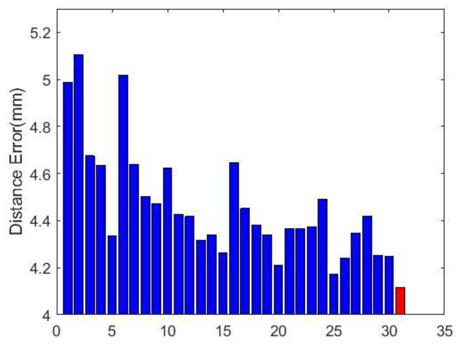
Landmarks	SIFT	LBP	HOG	Deep Features
Outer left eyebrow	6.13 ± 3.97	6.45 ± 4.11	6.38 ± 4.37	4.76 ± 3.15
Middle left eyebrow	5.37 ± 2.15	4.95 ± 2.07	5.68 ± 3.62	3.43 ± 2.38
Inner left eyebrow	5.14 ± 3.23	5.28 ± 3.45	5.48 ± 2.08	2.96 ± 2.14
Inner right eyebrow	5.04 ± 2.78	5.18 ± 2.96	5.34 ± 3.05	2.93 ± 1.79
Middle right eyebrow	4.88 ± 2.86	5.03 ± 2.54	5.08 ± 2.86	3.41 ± 2.06
Outer right eyebrow	6.02 ± 3.50	5.97 ± 3.45	6.17 ± 3.74	4.83 ± 4.07
Outer left eye corner	4.16 ± 2.05	4.83 ± 2.36	4.97 ± 2.60	3.14 ± 2.17
Inner left eye corner	4.53 ± 2.53	4.12 ± 2.27	5.02 ± 3.10	2.62 ± 1.73
Inner right eye corner	3.71 ± 2.19	4.03 ± 2.30	4.34 ± 2.62	2.74 ± 1.24
Outer right eye corner	4.09 ± 2.51	3.89 ± 2.84	4.13 ± 2.74	2.82 ± 1.85
Nose saddle left	7.85 ± 4.03	7.71 ± 3.96	7.91 ± 4.07	4.13 ± 2.75
Nose saddle right	8.23 ± 4.29	8.35 ± 4.02	8.41 ± 4.72	4.69 ± 3.18
Left nose peak	3.54 ± 2.06	3.67 ± 2.17	3.97 ± 2.37	2.96 ± 2.24
Nose tip	3.84 ± 2.43	3.91 ± 2.59	4.01 ± 2.77	2.69 ± 1.95
Right nose peak	3.53 ± 2.34	3.81 ± 2.61	3.48 ± 2.22	2.74 ± 2.27
Left mouth corner	4.39 ± 2.82	4.13 ± 2.58	4.47 ± 3.01	2.93 ± 3.24
Upper lip outer middle	4.73 ± 3.12	4.99 ± 3.19	4.45 ± 3.08	2.66 ± 2.63
Right mouth corner	6.32 ± 3.83	6.41 ± 3.95	7.04 ± 4.37	3.18 ± 2.93
Upper lip inner middle	4.86 ± 2.75	4.64 ± 2.67	4.93 ± 3.15	2.92 ± 2.65
Lower lip inner middle	5.15 ± 5.02	5.61 ± 4.96	5.89 ± 5.12	3.07 ± 3.17
Lower lip outer middle	6.19 ± 4.19	6.20 ± 3.95	6.07 ± 4.12	3.51 ± 3.15
Chin middle	7.69 ± 5.39	7.93 ± 5.62	8.01 ± 5.70	4.99 ± 4.16
Mean error	5.25 ± 3.18	5.32 ± 3.21	5.51 ± 3.43	3.37 ± 2.72

shows the average location error across all of the 22 landmarks on the Bosphporus database. We can easily draw the conclusion that the deep feature fusion marked with the bold fonts based on the pre-trained model is more accurate than the handcrafted features for all of these 22 landmarks. Furthermore, among these handcrafted features, the SIFT feature achieves the best performance, and outperforms HOG and LBP. These results also indicate that the location performance would obviously be affected by different features.

4.7.2. Comparison with Pre-Trained Models

This section compares the performance of deep fused features based on three different pre-trained models on the ImageNet dataset [43,44,45]. As aforementioned, different features extracted by using different pre-trained models were fed into the coarse-to-fine networks separately. In this paper, the same as the other handcrafted features, we use these pre-trained models to extract features from these facial attribute maps independently and fuse these features to train the designed model. Limited to numbers of the data, we keep all parameters fixed except the last fully connected layer. We only tested three classical deep models, including AlexNet [44], VGG-net [43] and Google Inception [45].

Table 2. Comparison with pre-trained deep models on BoshporusDB.

landmarks	AlexNet	Google Inception	VGG-Net
Outer left eyebrow	4.93 ± 2.54	4.47 ± 2.31	4.76 ± 3.15
Middle left eyebrow	4.19 ± 3.18	3.62 ± 2.47	3.43 ± 2.38
Inner left eyebrow	3.05 ± 2.43	2.88 ± 2.04	2.96 ± 2.14
Inner right eyebrow	3.16 ± 2.17	3.04 ± 1.92	2.93 ± 1.79
Middle right eyebrow	3.61 ± 2.58	3.55 ± 1.99	3.41 ± 2.06
Outer right eyebrow	4.02 ± 4.16	4.23 ± 4.35	4.83 ± 4.07
Outer left eye corner	3.16 ± 2.00	3.46 ± 2.10	3.14 ± 2.17
Inner left eye corner	2.39 ± 1.60	2.30 ± 1.40	2.62 ± 1.73
Inner right eye corner	3.10 ± 2.49	2.87 ± 1.54	2.74 ± 1.24
Outer right eye corner	3.01 ± 2.05	2.77 ± 1.94	2.82 ± 1.85
Nose saddle left	4.61 ± 3.56	4.88 ± 3.67	4.13 ± 2.75
Nose saddle right	5.71 ± 4.13	5.30 ± 3.71	4.69 ± 3.18
Left nose peak	3.51±2.99	3.11 ± 2.69	2.96 ± 2.24
Nose tip	3.31 ± 2.21	3.01 ± 2.07	2.69 ± 1.95
Right nose peak	2.56 ± 2.04	2.88 ± 2.50	2.74 ± 2.27
Left mouth corner	4.10 ± 3.74	3.43 ± 3.34	2.93 ± 3.24
Upper lip outer middle	3.29 ± 3.01	2.97 ± 2.85	2.66 ± 2.63
Right mouth corner	4.19 ± 3.45	3.57 ± 3.22	3.18 ± 2.93
Upper lip inner middle	3.61 ± 3.42	2.87 ± 3.15	2.92 ± 2.65
Lower lip inner middle	4.15 ± 5.04	3.59 ± 4.13	3.07 ± 3.17
Lower lip outer middle	4.19 ± 3.89	3.81 ± 3.77	3.51 ± 3.15
Chin middle	5.05 ± 5.04	5.13 ± 5.13	4.99 ± 4.16
Mean error	3.77 ± 3.08	3.53 ± 2.83	3.37 ± 2.72

shows the average location errors across all of the 22 landmarks on the Bosphorus database. The best performance is marked by bold fonts. From it, we can conclude that: (1) all of the deep features achieve better performance than the handcrafted features; (2) Deep fusion features all can achieve satisfied performance; and the (3) Google Inception network and AlexNet outperform the VGG-net for a few landmarks. However, comparing with VGG-net, Inception net takes too much time to extract features because of the complex architecture, and AlexNex is unsatisfactory among most of landmarks. Considering the computation accuracy and time complexity, the VGG-net has been chosen as the pre-trained deep model.

4.7.3. Comparison on the Bosphorus Dataset

Furthermore, we compared our proposed approach with other existing methods on the Bosphorus dataset. Figure 7 depicts the mean distance error and standard deviation of 22 detected landmarks. From this figure, the mean distance error of all landmarks in the testing data is $3.37$ mm, which has achieved the state-of-the-art, especially in some landmarks such as middle left/right eyebrow and so on. Compared with some other existing methods in these common landmarks, the comparison results are shown in

Table 3. Comparison with other methods on BoshporusDB.

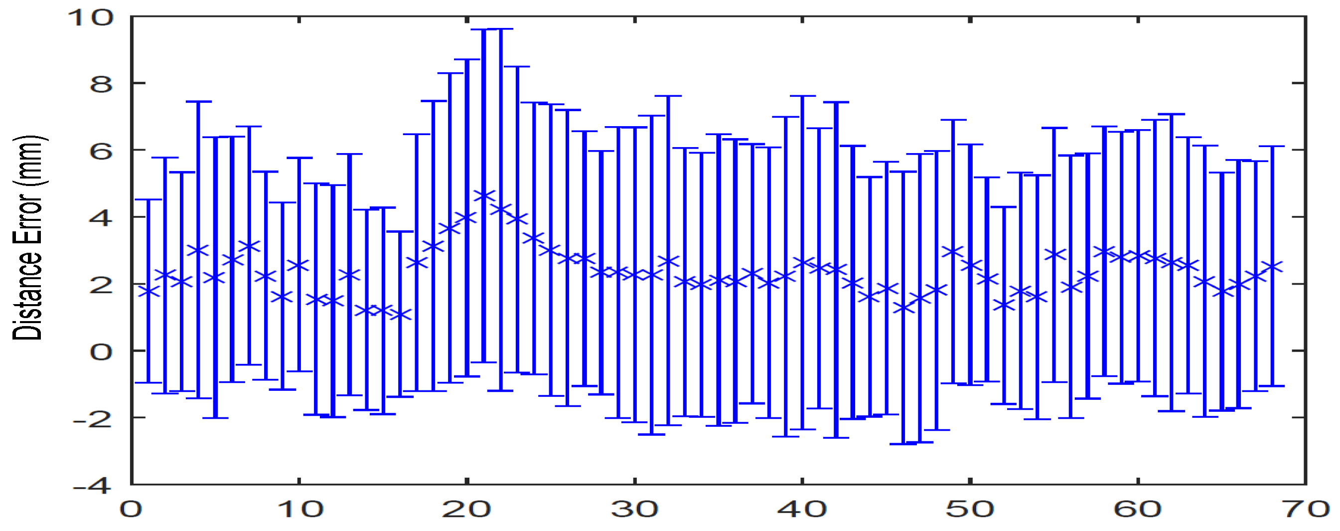
	Inner Eye Corners	Outer Eye Corners	Nose Tip	Nose Corners	Mouth Corners	Chin
Manual [46]	2.51	-	2.96	1.75	-	-
Alyuz [46]	3.70	-	3.05	3.10	-	-
Creusot [47]	4.14 ± 2.63	6.27 ± 3.98	4.33 ± 2.62	4.16 ± 2.35	7.95 ± 5.44	15.38 ± 10.49
Sukno [48]	2.85 ± 2.02	5.06 ± 3.67	2.33 ± 1.78	3.02 ± 1.91	6.08 ± 5.13	7.58 ± 6.72
Camgoz (SIFT) [49]	2.26 ± 1.79	4.23 ± 2.94	2.72 ± 2.19	4.57 ± 3.62	3.14 ± 2.71	5.72 ± 4.31
Camgoz (HOG) [49]	2.33 ± 1.92	4.11 ± 3.01	2.69 ± 2.20	4.49 ± 3.62	3.16 ± 2.70	5.87 ± 4.19
Ours	2.66 ± 1.49	3.64 ± 2.01	2.69 ± 1.95	4.40 ± 2.61	3.06 ± 3.09	4.99 ± 4.16

. The best performance is marked by bold fonts. From it, we can see that our approach outperforms in outer eye corners, chin and mouth corners, which are difficult to locate. Figure 8 illustrates some examples of facial landmarking by the proposed approach on this dataset. In this figure, 3D facial geometry data are rotated through several directions, so that the performance of landmarking can be observed more clearly.

4.7.4. Comparison on the BU-3DFE Dataset

The second experiment is carried out on the BU-3DFE dataset. Among the 2500 facial geometry data, 2000 facial scans from the 100 subjects were selected as the training data. The other 500 facial geometry data were used as testing data. After data argumentation, 12,000 facial scans can be obtained that contain neural expressions and six universal facial expressions. Figure 9 illustrates average distance error and standard deviation of 68 landmarks in the testing dataset of the 68 landmarks. Meanwhile, $98.88\%$ of the landmarks are located with a 20 mm precision, and $93.20\%$ are with the 10 mm precision. The mean distance error of all 68 landmarks has been improved to $4.03$ mm. Compared with some other methods in the common landmarks on BU-3DFE dataset,

Table 4. Comparison results with existing methods on BU3DFE.

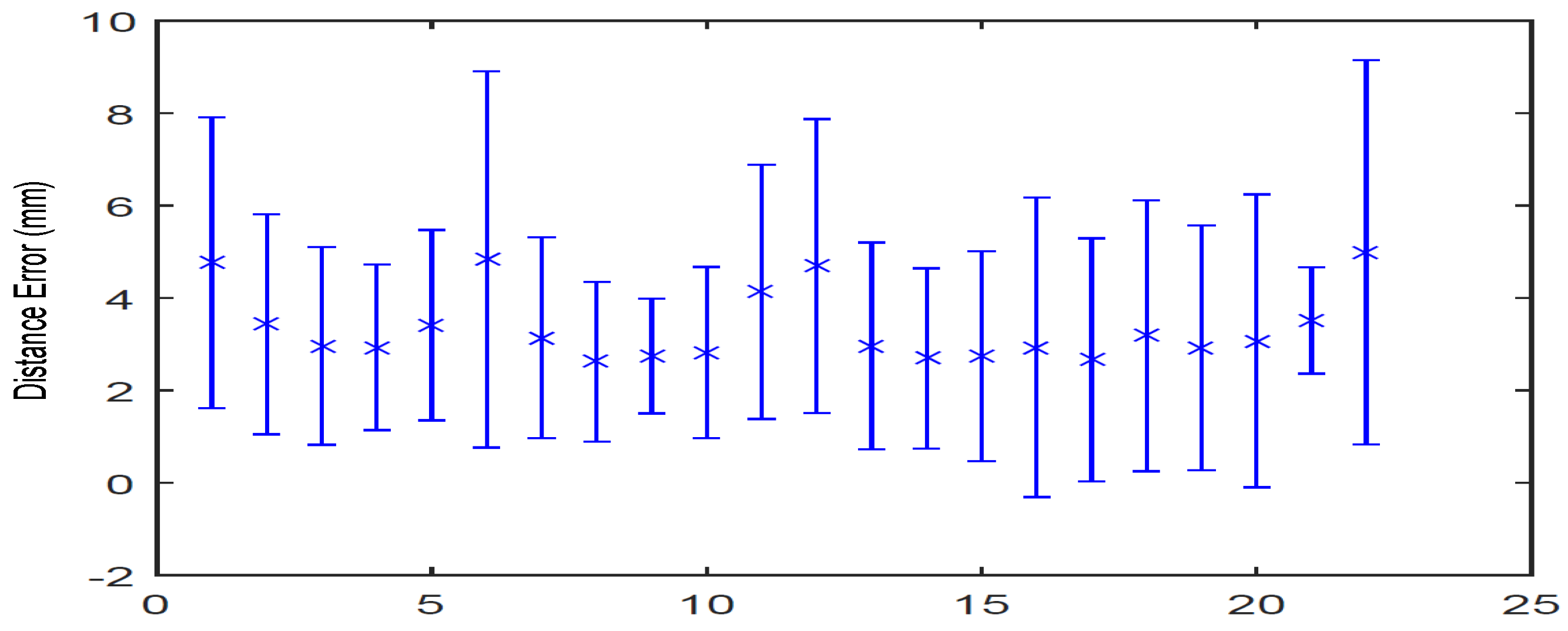
Landmark	Fanelli [50]	Zhao [20]	Nair [21]	Sun [51]	Our Method
Inner corner of left eye	2.60 ± 1.80	2.93 ± 1.40	11.89	3.35 ± 5.67	2.79 ± 1.63
Outer corner of left eye	3.60 ± 2.40	4.11 ± 1.89	19.38	3.89 ± 6.38	3.58 ± 2.27
Inner corner of right eye	2.80 ± 2.00	2.90 ± 1.36	12.11	3.27 ± 5.51	3.11 ± 2.24
Outer corner of right eye	4.00 ± 2.80	4.07 ± 2.00	20.46	3.73 ± 6.14	4.20 ± 2.18
Left corner of nose	3.90 ± 2.00	3.32 ± 1.94	-	3.60 ± 4.01	3.77 ± 1.87
Right corner of nose	4.10 ± 2.20	3.62 ± 1.91	-	3.43 ± 3.74	4.98 ± 2.63
Left corner of mouth	4.70 ± 3.50	7.15 ± 4.64	-	3.95 ± 4.17	3.88 ± 2.86
center of upper lip	3.50 ± 2.50	4.19 ± 2.34	-	3.09 ± 3.06	2.94 ± 1.35
Right corner of mouth	4.90 ± 3.60	7.52 ± 4.57	-	3.76 ± 4.05	3.94 ± 2.96
Center of lower lip	5.20 ± 5.20	8.82 ± 7.12	-	4.36 ± 6.03	3.73 ± 2.97
Outer corner of left brow	5.80 ± 3.80	6.26 ± 3.72	-	5.29 ± 6.93	4.92 ± 2.69
Inner corner of left brow	3.80 ± 2.70	4.87 ± 2.99	-	4.62 ± 5.92	3.81 ± 2.75
Inner corner of right brow	4.00 ± 3.00	4.88 ± 2.97	-	4.59 ± 5.76	3.85 ± 2.63
Outer corner of right brow	6.20 ± 4.30	6.07 ± 3.35	-	5.29 ± 7.04	5.98 ± 4.63
Mean results	4.22 ± 2.99	5.05 ± 3.01	-	4.02 ± 5.32	3.96 ± 2.55

depicts the comparison results of 14 common landmarks. The best performance is marked by bold fonts. We can see that the average error of these points has been achieved $3.96$mm and the results in several points outperform, including the outer corner of the left eye, center of the upper lip, and center of the lower lip.

5. Discussion

With the development of deep learning, more and more data is needed to train a robust and accurate model. Unlike 2D images that can be easily obtained from the web, the 3D geometry data can’t be constructed easily without professional equipment. Nowadays, the existing 3D geometry databases are all collected from labs and under the controlled conditions. Furthermore, the number of data is far from enough to train an appropriate deep model, so we need to fine-tune the pre-trained model. In this paper, using the pre-trained deep model to extract features from the different attribute maps is essential in the proposed approach. In most of the cases, fine-tuning these deep models means that most of the parameters in the pre-trained models remain unchanged and only a few are updated for specific tasks. For this purpose, we can update the parameters in the last layer or other layers based on the amount of training data. Thus, in our paper, limited to the number of 3D geometry data, we only updated the last layer and didn’t test the other choices at all.

In addition, feature fusion is the key step in the proposed approach. Applying the fused feature extracted from deep model can take more useful information into account for locating landmarks. For 3D data, more useful information can be obtained including surface normal, curvature and other attribute maps. In this paper, we only select these five types of attribute maps to train the model. In fact, for each attribute map, the features can be extracted based on different pre-trained models. It is another way to improve the location performance, but it is too complex to be applied in the other testing data satisfied. On the other hand, a classical pre-trained model named ResNet was not considered because of the computational complexity and our computer performance. Although the model would achieve the best performance for our task perhaps, it still cost more than 3 min to extract the features without updating any parameters. For this reason, ResNet was not selected in our approach.

As other research about deep learning, the main weakness is also the computation complexity. Compared with other effective approaches, the computation complexity of our proposed method is higher than the others. In addition, this paper is the first time to utilize the deep-learning based approach to estimate 3D landmarks, while the other effective methods are all based on traditional ways such as hand-crafted features. Actually, to improve the accuracy, higher computation complexity is needed. Benefiting from more and more powerful computing power, the execution time is still satisfied. Of course, a lot of works will be done to reduce the computation complexity and to ensure the accuracy improvement synchronously in future works.

Although our algorithm has achieved state-of-the-art performance, there are a few other works to study. Firstly, we didn’t take the profile face into account because there are only a few 3D profile data and fewer landmarks to train a unified location architecture. In addition, data missing caused by posing is the most challenging issue and the main weakness of our algorithm.

6. Conclusions

In this paper, we propose a novel approach to estimate landmarks on 3D geometry data. By transforming the 3D data to 2D attribute maps, the goal of our approach is to predict the landmarks based on the attribute maps. Different from using the handcrafted feature, we feed the global and the local attribute maps into the deep CNN model to extract global and local feature. Based on coarse-to-fine strategy, a global model is trained to estimate landmarks roughly and local models are trained to refine the landmarks’ location. Evaluated on the Bosphorus dataset, the proposed method performs more effectively than handcrafted features and other pre-trained models. Compared with other existing methods, the results on the Bosphorus dataset and BU-3DFE dataset have also demonstrated comparable performance, especially in some common landmarks.

In the future, some other issues of improving the robustness under other challenging conditions such as self-occlusion and data missing will be studied. In addition, using decision fusion of simple classifiers to balance the computation complexity and the accuracy may be another effective method for this problem.

References

- Cootes, T.F.; Edwards, G.J.; Taylor, C.J. Active Appearance Models. IEEE Trans. Pattern Anal. Mach. Intell. 2001, 23, 681–685. [Google Scholar] [CrossRef]
- Cootes, T.F.; Taylor, C.J.; Cooper, D.H.; Graham, J. Active shape models—Their training and application. Comput. Vis. Image Underst. 1995, 61, 38–59. [Google Scholar] [CrossRef]
- Cristinacce, D.; Cootes, T.F. Feature Detection and Tracking with Constrained Local Models. In Proceedings of the British Machine Vision Conference 2006, Edinburgh, UK, 4–7 September 2006; pp. 929–938. [Google Scholar]
- Kazemi, V.; Sullivan, J. One Millisecond Face Alignment with an Ensemble of Regression Trees. In Proceedings of the IEEE Conference on Computer Vision and Pattern Recognition, Columbus, OH, USA, 23–28 June 2014; pp. 1867–1874. [Google Scholar]
- Ren, S.; Cao, X.; Wei, Y.; Sun, J. Face Alignment at 3000 FPS via Regressing Local Binary Features. In Proceedings of the IEEE Conference on Computer Vision and Pattern Recognition, Columbus, OH, USA, 23–28 June 2014; pp. 1685–1692. [Google Scholar]
- Xiong, X.; Torre, F.D.L. Supervised Descent Method and Its Applications to Face Alignment. In Proceedings of the IEEE Conference on Computer Vision and Pattern Recognition, Portland, OR, USA, 23–28 June 2013; pp. 532–539. [Google Scholar]
- Dollar, P.; Welinder, P.; Perona, P. Cascaded pose regression. In Proceedings of the Computer Vision and Pattern Recognition, San Francisco, CA, USA, 13–18 June 2010; pp. 1078–1085. [Google Scholar]
- Savran, A.; Sankur, B.; Bilge, M.T. Regression-based intensity estimation of facial action units. Image Vis. Comput. 2012, 30, 774–784. [Google Scholar] [CrossRef]
- Feng, Z.H.; Huber, P.; Kittler, J.; Christmas, W.; Wu, X.J. Random Cascaded-Regression Copse for Robust Facial Landmark Detection. IEEE Signal Process. Lett. 2014, 22, 76–80. [Google Scholar] [CrossRef]
- Zhu, S.; Li, C.; Chen, C.L.; Tang, X. Face alignment by coarse-to-fine shape searching. In Proceedings of the Computer Vision and Pattern Recognition, Boston, MA, USA, 7–12 June 2015; pp. 4998–5006. [Google Scholar]
- Zhu, X.; Lei, Z.; Liu, X.; Shi, H.; Li, S.Z. Face Alignment Across Large Poses: A 3D Solution. In Proceedings of the IEEE Conference on Computer Vision and Pattern Recognition, Las Vegas, NV, USA, 27–30 June 2016; pp. 146–155. [Google Scholar]
- Jourabloo, A.; Liu, X. Pose-Invariant 3D Face Alignment. In Proceedings of the IEEE International Conference on Computer Vision, Santiago, Chile, 11–18 December 2016; pp. 3694–3702. [Google Scholar]
- Kakadiaris, I.A.; Passalis, G.; Toderici, G.; Murtuza, M.N.; Lu, Y.; Karampatziakis, N.; Theoharis, T. Three-dimensional face recognition in the presence of facial expressions: An annotated deformable model approach. IEEE Trans. Pattern Anal. Mach. Intell. 2007, 29, 640. [Google Scholar] [CrossRef] [PubMed]
- Perakis, P.; Theoharis, T.; Passalis, G.; Kakadiaris, I.A. Automatic 3D facial region retrieval from multi-pose facial datasets. In Proceedings of the Eurographics Conference on 3D Object Retrieval, Munich, Germany, 29 March 2009; pp. 37–44. [Google Scholar]
- Perakis, P.; Passalis, G.; Theoharis, T.; Toderici, G.; Kakadiaris, I.A. Partial matching of interpose 3D facial data for face recognition. In Proceedings of the IEEE International Conference on Biometrics: Theory, Applications, and Systems, Washington, DC, USA, 28–30 September 2009; pp. 1–8. [Google Scholar]
- Xu, C.; Tan, T.; Wang, Y.; Quan, L. Combining local features for robust nose location in 3D facial data. Pattern Recognit. Lett. 2006, 27, 1487–1494. [Google Scholar] [CrossRef]
- D’Hose, J.; Colineau, J.; Bichon, C.; Dorizzi, B. Precise Localization of Landmarks on 3D Faces using Gabor Wavelets. In Proceedings of the IEEE International Conference on Biometrics: Theory, Applications, and Systems, Crystal City, VA, USA, 27–29 September 2007; pp. 1–6. [Google Scholar]
- Colbry, D.; Stockman, G.; Jain, A. Detection of Anchor Points for 3D Face Veri.cation. In Proceedings of the IEEE Computer Society Conference on Computer Vision and Pattern Recognition, San Diego, CA, USA, 20–25 June 2005. [Google Scholar]
- Bevilacqua, V.; Casorio, P.; Mastronardi, G. Extending Hough Transform to a Points’ Cloud for 3D-Face Nose-Tip Detection. In Proceedings of the International Conference on Intelligent Computing: Advanced Intelligent Computing Theories and Applications—With Aspects of Artificial Intelligence, Shanghai, China, 15–18 September 2008; pp. 1200–1209. [Google Scholar]
- Zhao, X.; Dellandréa, E.; Chen, L.; Kakadiaris, I.A. Accurate landmarking of three-dimensional facial data in the presence of facial expressions and occlusions using a three-dimensional statistical facial feature model. IEEE Trans. Syst. Man Cybern. Part B Cybern. 2011, 41, 1417–1428. [Google Scholar] [CrossRef] [PubMed]
- Nair, P.; Cavallaro, A. 3-D Face Detection, Landmark Localization, and Registration Using a Point Distribution Model. IEEE Trans. Multimedia 2009, 11, 611–623. [Google Scholar] [CrossRef] [Green Version]
- Jahanbin, S.; Choi, H.; Jahanbin, R.; Bovik, A.C. Automated facial feature detection and face recognition using Gabor features on range and portrait images. In Proceedings of the IEEE International Conference on Image Processing, San Diego, CA, USA, 12–15 October 2008; pp. 2768–2771. [Google Scholar]
- Huibin, L.I.; Sun, J.; Zongben, X.U.; Chen, L. Multimodal 2D+3D Facial Expression Recognition with Deep Fusion Convolutional Neural Network. IEEE Trans. Multimedia 2017, 19, 2816–2831. [Google Scholar]
- Schroff, F.; Kalenichenko, D.; Philbin, J. FaceNet: A unified embedding for face recognition and clustering. In Proceedings of the IEEE Conference on Computer Vision and Pattern Recognition, Boston, MA, USA, 7–12 June 2015; pp. 815–823. [Google Scholar]
- Sun, Y.; Liang, D.; Wang, X.; Tang, X. DeepID3: Face Recognition with Very Deep Neural Networks. arXiv, 2015; arXiv:1502.00873. [Google Scholar]
- Taigman, Y.; Yang, M.; Ranzato, M.; Wolf, L. DeepFace: Closing the Gap to Human-Level Performance in Face Verification. In Proceedings of the Computer Vision and Pattern Recognition, Columbus, OH, USA, 23–28 June 2014; pp. 1701–1708. [Google Scholar]
- Chang, F.J.; Tran, A.T.; Hassner, T.; Masi, I.; Nevatia, R.; Medioni, G. ExpNet: Landmark-Free, Deep, 3D Facial Expressions. In Proceedings of the 2018 13th IEEE International Conference on Automatic Face & Gesture Recognition (FG 2018), Xi’an, China, 15–19 May 2018. [Google Scholar]
- Sun, Y.; Wang, X.; Tang, X. Deep Convolutional Network Cascade for Facial Point Detection. In Proceedings of the Computer Vision and Pattern Recognition, Portland, OR, USA, 23–28 June 2013; pp. 3476–3483. [Google Scholar]
- Zhang, J.; Shan, S.; Kan, M.; Chen, X. Coarse-to-Fine Auto-Encoder Networks (CFAN) for Real-Time Face Alignment. In European Conference on Computer Vision; Springer: Cham, Switzerland, 2014; pp. 1–16. [Google Scholar]
- Zhang, Z.; Luo, P.; Chen, C.L.; Tang, X. Facial Landmark Detection by Deep Multi-task Learning. In Proceedings of the European Conference on Computer Vision, Zurich, Switzerland, 6–12 September 2014; pp. 94–108. [Google Scholar]
- Yang, J.; Liu, Q.; Zhang, K. Stacked Hourglass Network for Robust Facial Landmark Localisation. In Proceedings of the Computer Vision and Pattern Recognition Workshops, Honolulu, HI, USA, 21–26 July 2017; pp. 2025–2033. [Google Scholar]
- Kumar, A.; Chellappa, R. Disentangling 3D Pose in A Dendritic CNN for Unconstrained 2D Face Alignment. In Proceedings of the IEEE Conference on Computer Vision and Pattern Recognition, Salt Lake City, UT, USA, 18–22 June 2018. [Google Scholar]
- Bulat, A.; Tzimiropoulos, G. How Far are We from Solving the 2D and 3D Face Alignment Problem? (and a Dataset of 230,000 3D Facial Landmarks). In Proceedings of the International Conference on Computer Vision, Venice, Italy, 22–29 October 2017; pp. 1021–1030. [Google Scholar]
- Lu, X.; Jain, A.K.; Colbry, D. Matching 2.5D Face Scans to 3D Models. IEEE Trans. Pattern Anal. Mach. Intell. 2006, 28, 31–43. [Google Scholar] [PubMed]
- Dibeklioglu, H.; Salah, A.A.; Akarun, L. 3D Facial Landmarking under Expression, Pose, and Occlusion Variations. In Proceedings of the IEEE International Conference on Biometrics: Theory, Applications and Systems, Arlington, VA, USA, 29 September–1 October 2008; pp. 1–6. [Google Scholar]
- Colombo, A.; Cusano, C.; Schettini, R. 3D face detection using curvature analysis. Pattern Recognit. 2006, 39, 444–455. [Google Scholar] [CrossRef]
- Boehnen, C.; Russ, T. A Fast Multi-Modal Approach to Facial Feature Detection. In Proceedings of the Seventh IEEE Workshops on Application of Computer Vision, Breckenridge, CO, USA, 5–7 January 2005; pp. 135–142. [Google Scholar]
- Wang, Y.; Chua, C.S.; Ho, Y.K. Facial feature detection and face recognition from 2D and 3D images. Pattern Recognit. Lett. 2002, 23, 1191–1202. [Google Scholar] [CrossRef]
- Salah, A.A.; Çinar, H.; Akarun, L.; Sankur, B. Robust facial landmarking for registration. Ann. Télécommun. 2007, 62, 83–108. [Google Scholar]
- Lu, X.; Jain, A.K. Automatic Feature Extraction for Multiview 3D Face Recognition. In Proceedings of the International Conference on Automatic Face and Gesture Recognition, Southampton, UK, 10–12 April 2006; pp. 585–590. [Google Scholar] [Green Version]
- Savran, A.; Akarun, L. Bosphorus Database for 3D Face Analysis. In Biometrics and Identity Management; Springer: Berlin/Heidelberg, Germany, 2008; pp. 47–56. [Google Scholar]
- Yin, L.; Wei, X.; Sun, Y.; Wang, J.; Rosato, M.J. A 3D facial expression database for facial behavior research. In Proceedings of the FGR’06 International Conference on Automatic Face and Gesture Recognition, Southampton, UK, 10–12 April 2006; pp. 211–216. [Google Scholar]
- Simonyan, K.; Zisserman, A. Very Deep Convolutional Networks for Large-Scale Image Recognition. arXiv, 2014; arXiv:1409.1556. [Google Scholar]
- Krizhevsky, A.; Sutskever, I.; Hinton, G.E. ImageNet classification with deep convolutional neural networks. In Proceedings of the International Conference on Neural Information Processing Systems, Doha, Qatar, 26–29 November 2012; pp. 1097–1105. [Google Scholar]
- Ioffe, S.; Szegedy, C. Batch Normalization: Accelerating Deep Network Training by Reducing Internal Covariate Shift. arXiv, 2015; arXiv:1502.03167. [Google Scholar]
- Alyüz, N.; Gökberk, B.; Akarun, L. Regional registration for expression resistant 3-D face recognition. IEEE Trans. Inf. Forensics Secur. 2010, 5, 425–440. [Google Scholar] [CrossRef]
- Creusot, C.; Pears, N.; Austin, J. A Machine-Learning Approach to Keypoint Detection and Landmarking on 3D Meshes. Int. J. Comput. Vis. 2013, 102, 146–179. [Google Scholar] [CrossRef]
- Sukno, F.M.; Waddington, J.L.; Whelan, P.F. 3-D Facial Landmark Localization With Asymmetry Patterns and Shape Regression from Incomplete Local Features. IEEE Trans. Cybern. 2017, 45, 1717–1730. [Google Scholar] [CrossRef] [PubMed]
- Camgöz, N.C.; Gökberk, B.; Akarun, L. Facial landmark localization in depth images using Supervised Descent Method. In Proceedings of the Signal Processing and Communications Applications Conference, Malatya, Turkey, 16–19 May 2015; pp. 378–383. [Google Scholar]
- Fanelli, G.; Dantone, M.; Gool, L.V. Real time 3D face alignment with Random Forests-based Active Appearance Models. In Proceedings of the IEEE International Conference and Workshops on Automatic Face and Gesture Recognition, Shanghai, China, 22–26 April 2013; pp. 1–8. [Google Scholar]
- Sun, J.; Huang, D.; Wang, Y.; Chen, L. A coarse-to-fine approach to robust 3D facial landmarking via curvature analysis and Active Normal Model. In Proceedings of the IEEE International Joint Conference on Biometrics, Clearwater, FL, USA, 29 September–2 October 2014; pp. 1–7. [Google Scholar]