No-Reference Image Blur Assessment Based on Response Function of Singular Values


1
School of Computer Science and Technology, Hangzhou Dianzi University, Hangzhou 310018, China
2
Department of Computer Science, University of Warwick, Coventry CV4 7AL, UK
*
Author to whom correspondence should be addressed.
Symmetry 2018, 10(8), 304; https://doi.org/10.3390/sym10080304
Submission received: 26 June 2018
/
Revised: 21 July 2018
/
Accepted: 23 July 2018
/
Published: 1 August 2018
(This article belongs to the Special Issue Information Technology and Its Applications 2021)
Abstract
:Blur is an important factor affecting the image quality. This paper presents an efficient no-reference (NR) image blur assessment method based on a response function of singular values. For an image, the grayscale image is computed to the acquire spatial information. In the meantime, the gradient map is computed to acquire the shape information, and the saliency map can be obtained by using scale-invariant feature transform (SIFT). Then, the grayscale image, the gradient map, and the saliency map are divided into blocks of the same size. The blocks of the gradient map are converted into discrete cosine transform (DCT) coefficients, from which the response function of singular values (RFSV) are generated. The sum of the RFSV are then utilized to characterize the image blur. The variance of the grayscale image and the DCT domain entropy of the gradient map are used to reduce the impact of the image content. The SIFT-dependent weights are calculated in the saliency map, which are assigned to the image blocks. Finally, the blur score is the normalized sum of the RFSV. Extensive experiments are conducted on four synthetic databases and two real blur databases. The experimental results indicate that the blur scores produced by our method are highly correlated with the subjective evaluations. Furthermore, the proposed method is superior to six state-of-the-art methods.
1. Introduction
The quality assessment of digital images has become an increasingly important issue in many modern multimedia systems, where various kinds of distortions are introduced during storage, compression, processing, and transmission. Based on the availability of the reference image, the existing image quality assessment (IQA) metrics are classified into three categories, full-reference (FR) metrics [1,2,3,4,5,6], reduced-reference (RR) metrics [7,8,9,10,11,12,13], and no-reference (NR) metrics [14,15,16,17,18,19,20,21,22,23]. By comparison, NR metrics have more applications in the real world, as the image quality of the distorted image can be assessed without any reference.
Blur is a major factor affecting the image quality. In the past few years, a series of NR assessment methods have been proposed. Blur is usually created by low pass filtering, which widens the edge of the image. Marziliano et al. [14] presented a method by detecting the width of the image edges in the spatial domain. First of all, the edges are extracted using Sobel edge detection operators. Then, the blur degree of the whole image is estimated by calculating the mean edge width. In the literature [15], Ferzli et al. presented a metric based on the just noticeable blur (JNB). The image local contrast and edge width are calculated as the inputs to a probability summation model, which produces the blur score. Narvekar et al. [16] introduced an approach based on JNB. The probability of detecting a blur is first estimated using a probabilistic model, then the blur score is produced by computing the cumulative probability of blur detection (CPBD). Vu et al. [17] presented the spectral and spatial sharpness (S3) model. Firstly, the attenuation of the high-frequency information is computed, and then the total variation (TV) model is utilized to estimate the change of contrast component on the blur image. The final blur score is calculated based on these features. In the literature [18], the metric predicted the image blur by using local phase coherence (LPC). The blur score is calculated in the transform domains. In the literature [19], Bahrami and Kot proposed to use the maximum local variation (MLV), which is computed within a small neighborhood for each pixel. The blur score is calculated by the standard deviation of the weighted MLV distribution. Kerous et al. [20] proposed a method using discrete cosine transform (DCT) and JNB. The edge map is obtained through the JNB method. Then, the blue score is computed based on a machine learning system. In the literature [21], the authors proposed a blind image blur evaluation (BIBLE) method based on Tchebichef moments [24], which was are to calculate the sum of the squared non-DC moment (SSM) values. SSM values are employed to estimate the degree of blur. In consideration of the effect of the image content, the sum of variances is employed to normalize the SSM values. Meanwhile, in order to generate a blur score close to HVS, the saliency detection by simple priors (SDSP) method [25] is employed to obtain the visually salient regions. Finally, the blur score is produced by normalizing the SSM values, which is assigned weights by the saliency map. Zhang et al. [22] introduced a novel metric based on SIFT and DCT. Some interested blocks are determined based on scale-invariant feature transform (SIFT) technology. Then, the sum of the squared AC coefficients of the DCT (SSAD) of the corresponding block is calculated to represent the extent of the blur. Considering of the impact of the image content, the sum of block variances and entropy are used to normalize the final blur score.
Although the method in the literature [22] showed the good results on four synthetic blur databases, this method did not achieve good performances for the real blur images. First of all, as the qualities of the real blurred images are usually determined by many factors, the sum of the SSAD does not suffice to represent the extent of the blur. In response to this, we use a difference matrix to analyze the change between the DCT coefficients, singular values to represent this change, and a response function of the singular values to estimate the image blur. Secondly, the image content is generally affected by many factors, such as variance and entropy. As the DCT domain entropy is important spectral information, we combine the variance of the original image and the DCT domain entropy, in order to reduce the impact of the image content.
As aforementioned, the previous methods cannot produce good results simultaneously on both the synthetic blur databases and real blur databases. In this paper, an efficient NR image blur evaluation metric is presented, which outperforms the state-of-the-art methods on both classes of databases. We utilize the singular values of the response function (PVRF) combining with the scale-invariant feature transform (SIFT) and the DCT domain entropy, in order to estimate the degree of blur in the images. Our method is motivated by the literature [12,22,26,27]. Sun et al. [12] proposed a novel NR image quality assessment method based on the SIFT intensity. In fact, the feature points can represent the sharpness of the image, and the number of feature points can reflect the image shape changes. In order to obtain the robust feature points, we select the SIFT points here, because of its multiscale characteristic. Meanwhile, the number of SIFT feature points is used to assign different weights. In the literature [26,27], an image is first divided into 8 × 8 blocks, and then these blocks are transformed to a DCT domain. Finally, the DCT domain entropies are calculated as the spectral features. We combine the variance and DCT domain entropy to normalize the sum of RFSV, and the final blur score is less affected by the image content in our experiment. Extensive experiments are made on four synthetic databases and two real blur databases. The experimental results indicate that our method is superior to the existing NR image quality assessment methods. The three main contributions of our method are as follows:
- We designed a response function of the singular values in the DCT domain, which is effective to characterize the image blur.
- We combine the spatial information of the blurred image and the spectral information of the gradient map, in order to reduce the impact of the image content.
- We assign SIFT-dependent weights to the image blocks, according to the characteristics of the human visual system (HVS).
2. The Proposed Methods
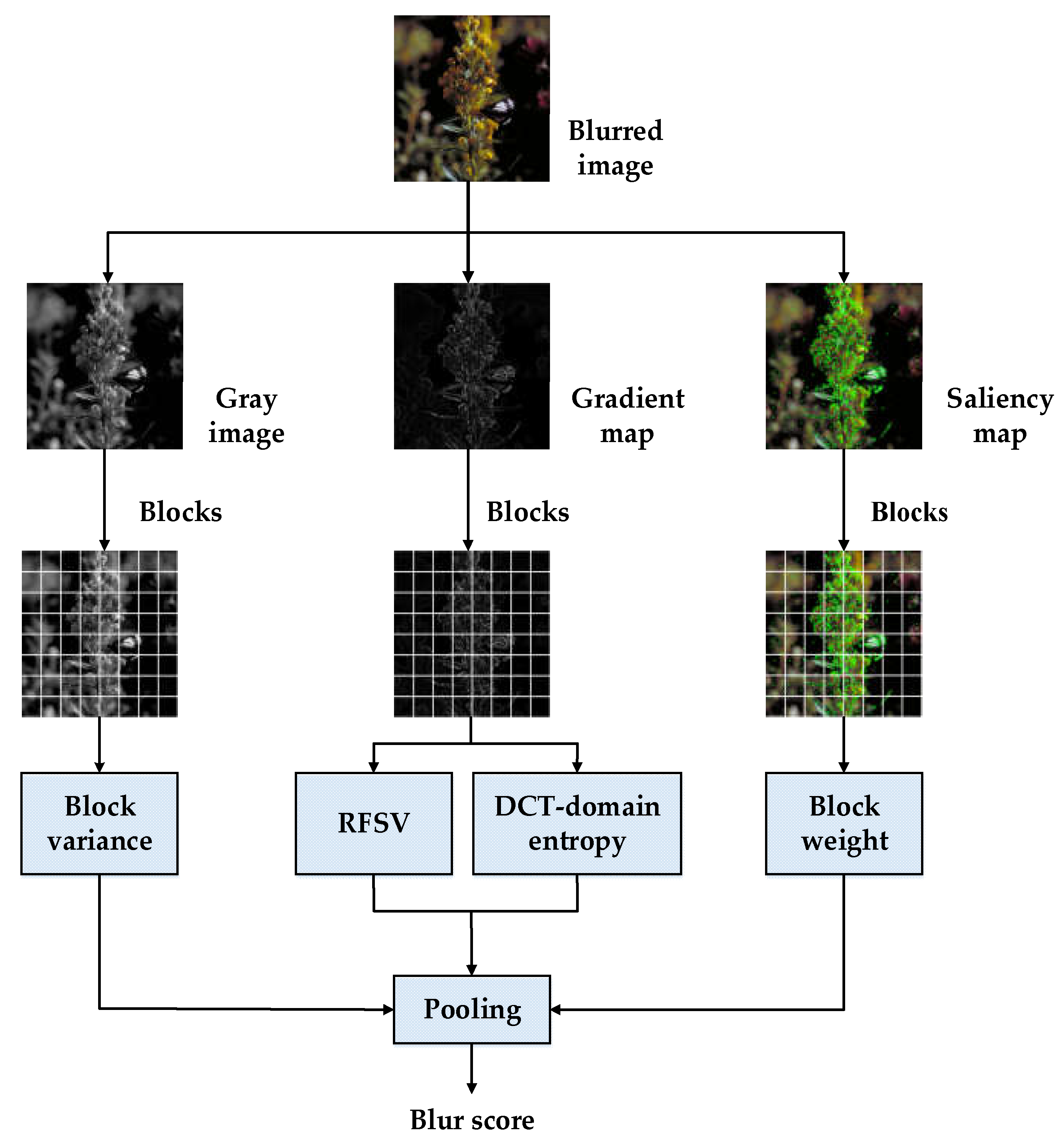
We propose a no-reference blur image assessment method based on the response function of the singular values in the DCT domain. The flowchart of our method is shown in Figure 1. It includes two phases; in the first phase, we calculate four components, as follows: (1) the RFSV for every block of the gradient map; (2) the variance for every block of the gray image; (3) the DCT domain entropy for every block of the gradient map; and (4) the block weight for every block of the saliency map. The sum of the RFSV is used to evaluate the blur degree. The sum of variances and the DCT domain entropy are used to normalize the sum of the RFSV. The block weight of the saliency map is designed to adapt to the characteristics of the HVS. In the second phase, we combine these four components to generate the final blur score.
2.1. Computing Gray Image and Gradient Map
To begin with, a blur image is converted to a grayscale image , where , . In order to acquire the shape information of the grayscale image, the gradient map is first calculated as follows:
where denotes the convolution and denotes the transpose.
Then, the grayscale image and the gradient map are divided into blocks of the same size. The block size is set to . The grayscale image block and the gradient block sets are denoted by and , respectively, where , , , , and is the floor operator.
2.2. Computing RFSV for Every Block
First of all, each gradient block in is converted into DCT domain, and denoted by the following:
where is the DC coefficient of a block, and the rest variables are the AC coefficients that reflect the image’s edges and shapes. By replacing the DC coefficient with 0, we obtain the following
Next, we estimate the blur degree from the DCT domain information of a block image. In order to analyze the change between the DCT coefficients, the horizontal and vertical direction difference values are calculated and are denoted, respectively, by the following:
where and , and
where and . and can be represented collectively as a difference matrix , as follows:
where (:) denotes a conversion from a matrix to a column, and is the length of the column.
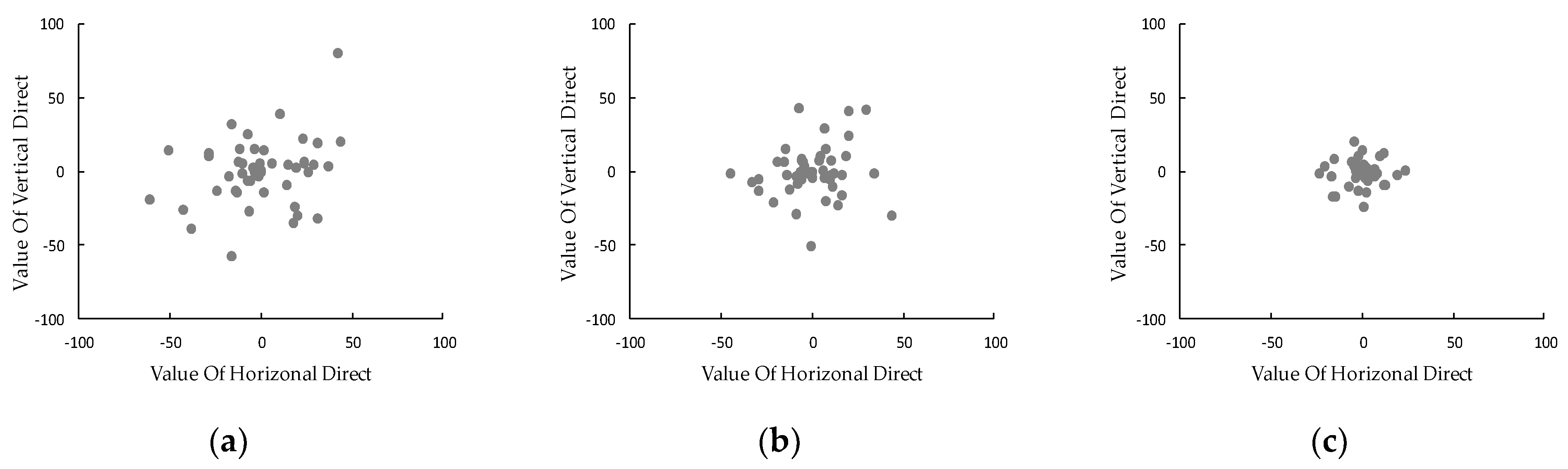
In order to illustrate the validity of the differential matrix to estimate the blur degree of the image, we plot (in Figure 2) the value of the difference matrix in the horizontal direction and vertical direction of a block under different blur degrees. One can observe from Figure 2a,b that the distribution of the scattered points is very scattered, which is due to the weak dependencies between and . The dependencies increase with a stronger Gaussian blur, resulting an approximately elliptical structure in Figure 2c, which concentrates around the zero values. The dependencies can be distinguished from the singular values of the difference matrices. The singular values are computed by singular value decomposition (SVD).
where and are the unitary matrices. The columns of and are the left and right singular vectors. is a diagonal matrix with the ordered singular values s1 and s2 (s1 > s2) on the diagonal. In order to demonstrate the validity of both singular values to capture the dependencies of the differential matrix elements, we select an image from the categorical subjective image quality (CSIQ) database [4]. Then, the singular values of each block are computed using Equation (8). In our experiment, we randomly select thirty blocks from the total blocks. The distribution of the singular values s1 and the singular values s2 of thirty blocks with different standard deviations of the Gaussian blur are shown in Figure 3.
It is shown in Figure 3 that the singular values, s1 and s2, of a block decrease with the increasing blur strength. If an image block is sharp, the singular values, s1 and s2, tend to be large. Inspired by the Harris corner detection, we design a response function of singular values (RFSV), as follows:
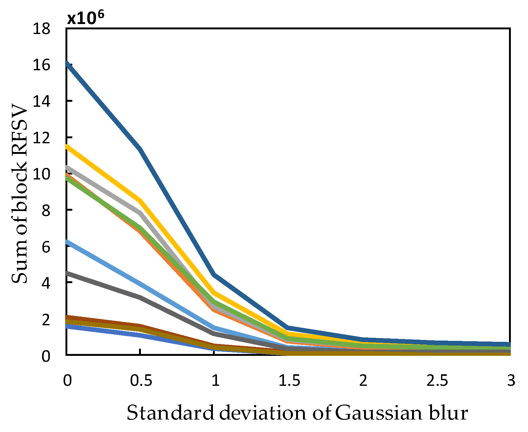
In Equation (9), is a RFSV of an image block. In our experiment, we set . Intuitively, if a block is blurred, the singular values, s1 and s2, tend to be small, and RFSV of the block will also be small. We can say that the RFSV is positively related to s1 and s2. Therefore, the sum of RFSV can estimate the degree of the blur within an image. An experiment is designed to prove this, we randomly select 10 undistorted images from the CSIQ database. The relation between the sum of the RFSV and the Gaussian blur standard deviation is shown in Figure 4. It is observed in Figure 4, that the sum of the RFSV of an image decreases significantly with the increasing standard deviation of the Gaussian blur.
2.3. Computing Variance and the DCT Domain Entropy for Every Block
The sum of the RFSV can be used to measure the blur degree of an image. However, from Figure 4, we discover that the sum of the RFSV of the different blur images are different, although they are at the same Gaussian blur degree. This is because the different blur images have different contents. In order to obtain similar blur scores of the images with the similar blur degree, we should minimize the impact of the image content.
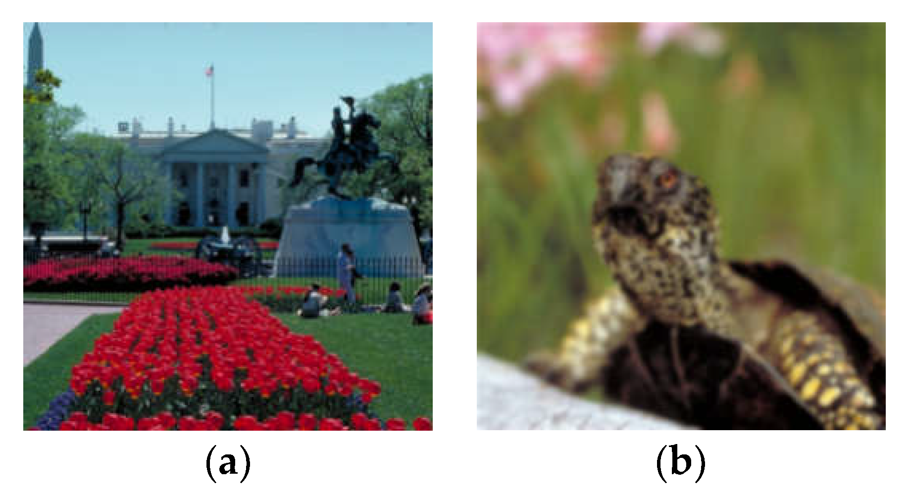
Li et al. [21] proposed to minimize the impact of the image content by using the sum of block variances, because of the fact that the different images have different variances. Zhang et al. [22] indicated that the use of variance is not enough to eliminate the effects of the image content completely, because some of the images with the almost equal variance may have different contents. Therefore, they proposed to add entropy on the basis of variance. However, we found that the images with different contents might have the same entropy. As shown in Figure 5, the entropies of the two images are both 7.23. Because the spatial information of the image (e.g., variance and entropy) are not enough to eliminate the effects of the image content completely, we should also consider the spectral information of the image.
The DCT domain entropy was employed to assess the image quality in the literature [26,27]. Different from the image entropy, the DCT domain entropy represents the probability distribution of the local DCT coefficients. We combine the variance and DCT domain entropy to normalize the sum of the RFSV, and as a result, the blur scores generated by our method are less affected by the image content. The variance and DCT domain entropy are defined by the following:
where denotes the variance of a block , and denotes the mean value of the corresponding block. Each DCT coefficient is normalized by the following:
and the DCT domain entropy of a local block is computed by the following:
2.4. Computing Block Weight
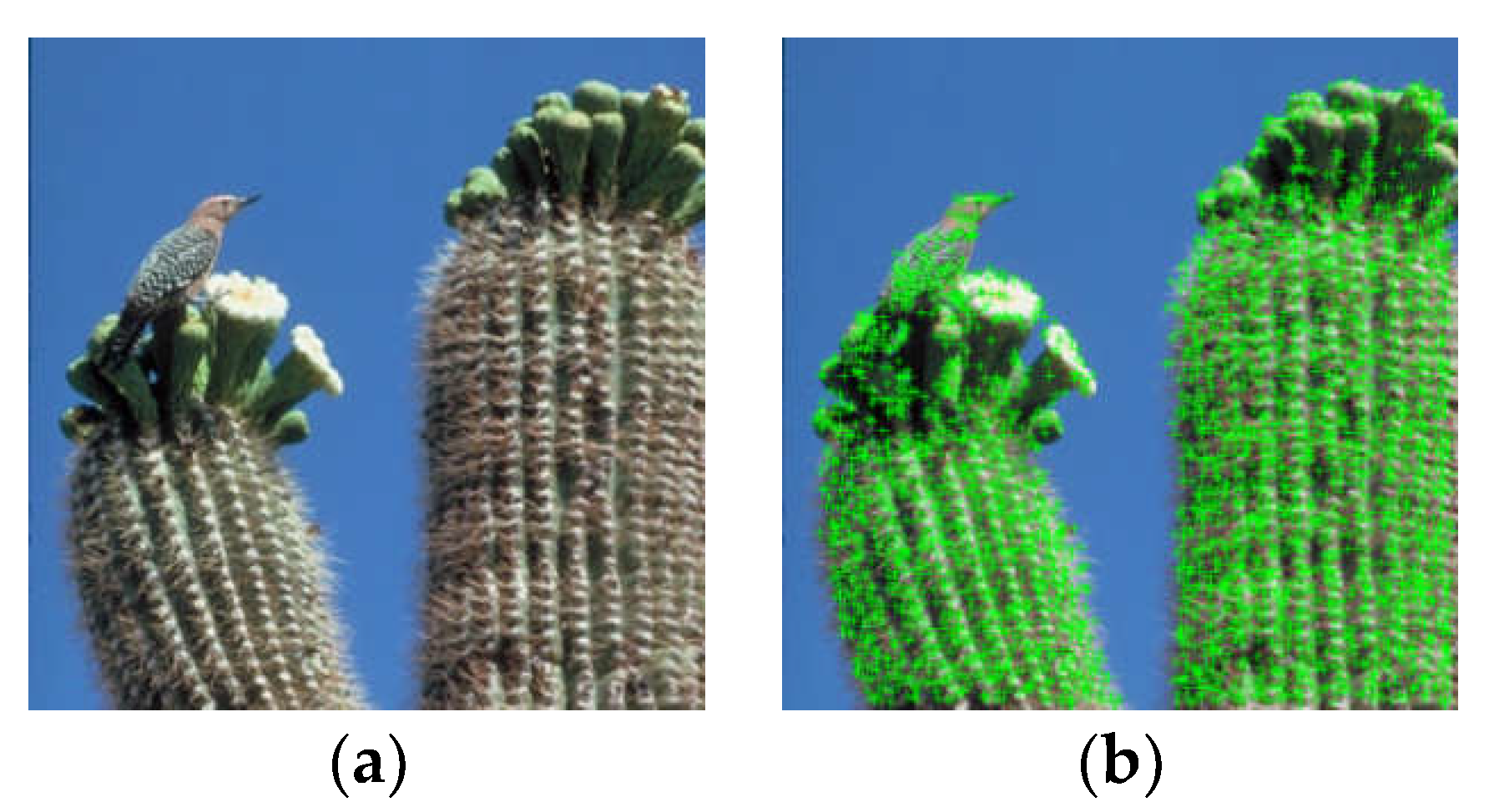
In practice, the visually salient regions are often used to estimate the sharpness of an image. For example, in Figure 6a, the visually salient region is the image’s foreground, rather than the blur background. If an image is sharp, the salient regions will also be sharp. Therefore, this characteristic is crucial to the final blur score. In the literature [12], the SIFT features were used to assess the image quality. In the literature [21], the SDSP model was used to generate a saliency map. In this paper, the saliency map is constructed using SIFT technology. Compared with the SDSP model, the SIFT technology has a lower time complexity and a higher accuracy. The saliency map in Figure 6b is detected from the blurred image in Figure 6a. It is observed that the SIFT points can accurately locate the visually salient regions. Therefore, the number of SIFT points is used to assign weights. We combine the visual saliency with the normalized sum of the RFSV to generate the blur score. The saliency map is divided into blocks of the same size. The saliency map blocks are denoted by , and the block weight denoted by , as follows:
where , , is the SIFT number of the block , and is a constant determined by experiments. The final blur score is denoted by the following:
where is the scale factor.
3. Results
3.1. Experimental Settings
In this section, six public image quality databases are used to estimate the performance of our method, including the laboratory for the image as well as the Video Engineering (LIVE) [28], CSIQ [4], Tampere Image Database 2008 (TID2008) [29], Tampere Image Database 2013 (TID2013) [30], Camera Image Database (CID2013) [31], and Blurred Image Database (BID) [32] . Among them, LIVE, CSIQ, TID2008, and TID2013 are synthetic blur databases, while CID2013 and BID are real blur databases. The images in the synthetic blur databases are generated using Gaussian low-pass filtering, and thus they aim to simulate the pure blur. By contrast, the real blur databases contain images captured by cameras in complex environments; in other words, they are distorted by multiple distortions. The number of blurred images that are tested on the six databases are 145, 150, 100, 125, 474, and 586, respectively. For each image in LIVE and CSIQ, human assessment scores are provided by a difference mean opinion score (DMOS), and for each image in TID2008, CID2013, TID2013, and BID, the human assessment scores are provided by the mean opinion score (MOS).
We compare the performance of our method with seven existing methods, JNB [15], CPBD [16], S3 [17], LPC [18], MLV [19], BIBLE [21], and Ref. [22]. Four common criterions are used as a reference, including the Pearson Linear Correlation Coefficient (PLCC), root mean square error (RMSE), Spearman Rank Order Correlation Coefficient (SRCC), and the Kendall rank order correlation coefficient (KRCC). SRCC and KRCC are employed for measuring the monotonicity. The PLCC and RMSE are employed to assess the prediction accuracy. In order to calculate these values, a nonlinear fitting function is needed to describe the relation between the predicted scores and the human assessment scores. In this paper, we employ a four-parameter logistic function, as follows:
where , , , and are the four fitting parameters. Typically, an excellent method produces high values of SRCC, KRCC, and PLCC, and low values of RMSE.
In implementation, the block size is , the scale factor is 0.1, the exponential of variance is 1, the exponential of the DCT domain entropy is 2, the parameter of response function is set with , and the parameter of the weight function is set with . Lowe’s Matlab source code is applied to detect the SIFT points, and the detailed configurations can be found in the literature [33].
3.2. Results and Analysis
3.2.1. Image-Level Evaluation
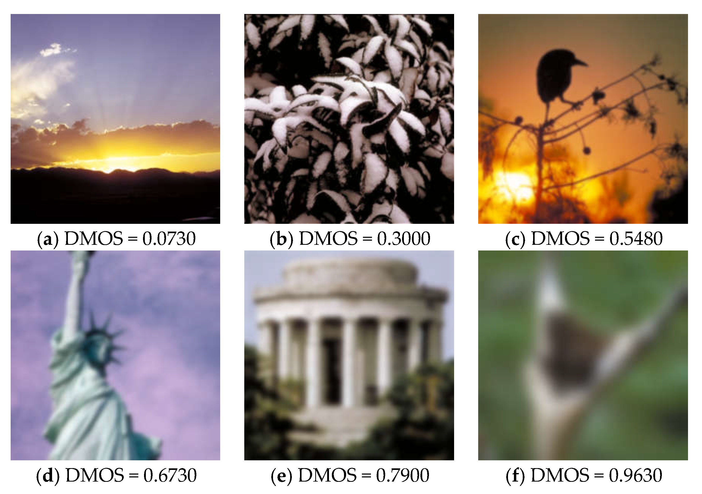
We test the proposed method with some blurred images. Six images with different blur degrees from the CSIQ database are shown in Figure 7. The human assessment scores are provided by DMOS, and the predicted blur scores generated by the proposed method as well as the seven existing blind image blur methods, including JNB [15], CPBD [16], S3 [17], LPC [18], MLV [19], BIBLE [21], and Ref. [22].
It is shown in Figure 7 that six images have increasing blur degrees. From Table 1, one can see that the blur scores generated by our method decrease drastically with the increasing blur degree. What’s more, our blur scores are consistent with the human assessment scores. By comparing with the seven existing methods, we find that LPC and Ref. [22] can generate scores that are consistent with the blur degree. However, the blur scores generated by the other metrics do not always make an accurate evaluation. The CPBD method generates incorrect scores between Figure 7d,e. Figure 7e has higher DMOS than Figure 7d, while the blur score of Figure 7d should be greater than the score of Figure 7e. The S3 and MLV methods generate incorrect scores between Figure 7b,c. According to the changes of the DMOS, the blur score for Figure 7c should be higher than the score for Figure 7b. The BIBLE and JNB methods have the same issue between Figure 7e,f.
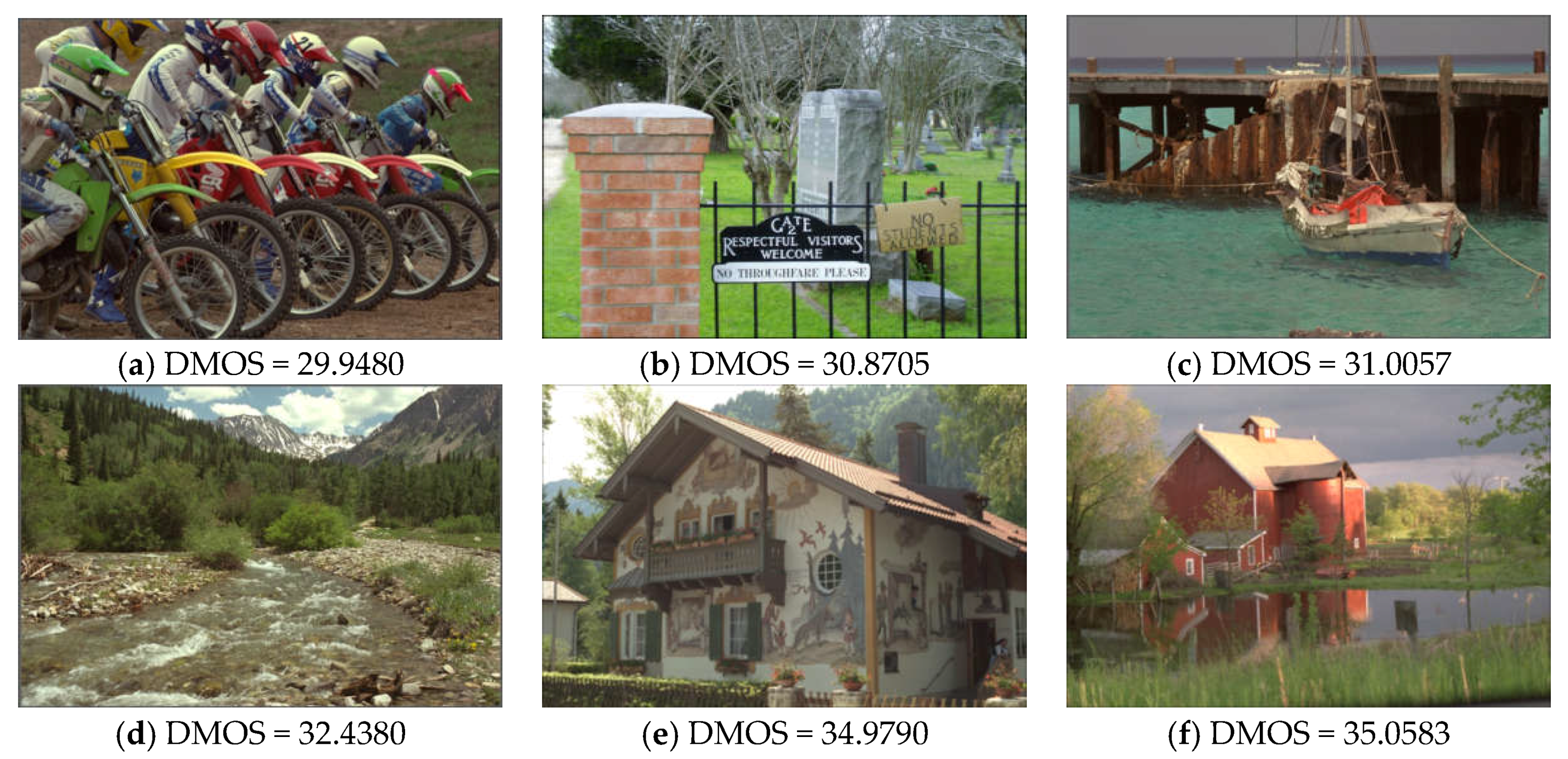
In the next experiment, we test our method with six images of the LIVE database. It is shown in Figure 8 that they all have similar blur degrees. Because the DMOS of these images monotonically increase, a good blind blur method is expected to generate the monotonically increasing or decreasing scores. Moreover, these blur scores should be nearly identical. The blur scores generated by different methods are summarized in Table 2.
From Table 2, our method can generate nearly identical and monotonically decreasing scores. However, the blur scores generated by other methods do not have better monotonicity. Therefore, our method effectively distinguishes the images with similar blur degrees, which are highly consistent with DMOS.
3.2.2. Database-Level Evaluation
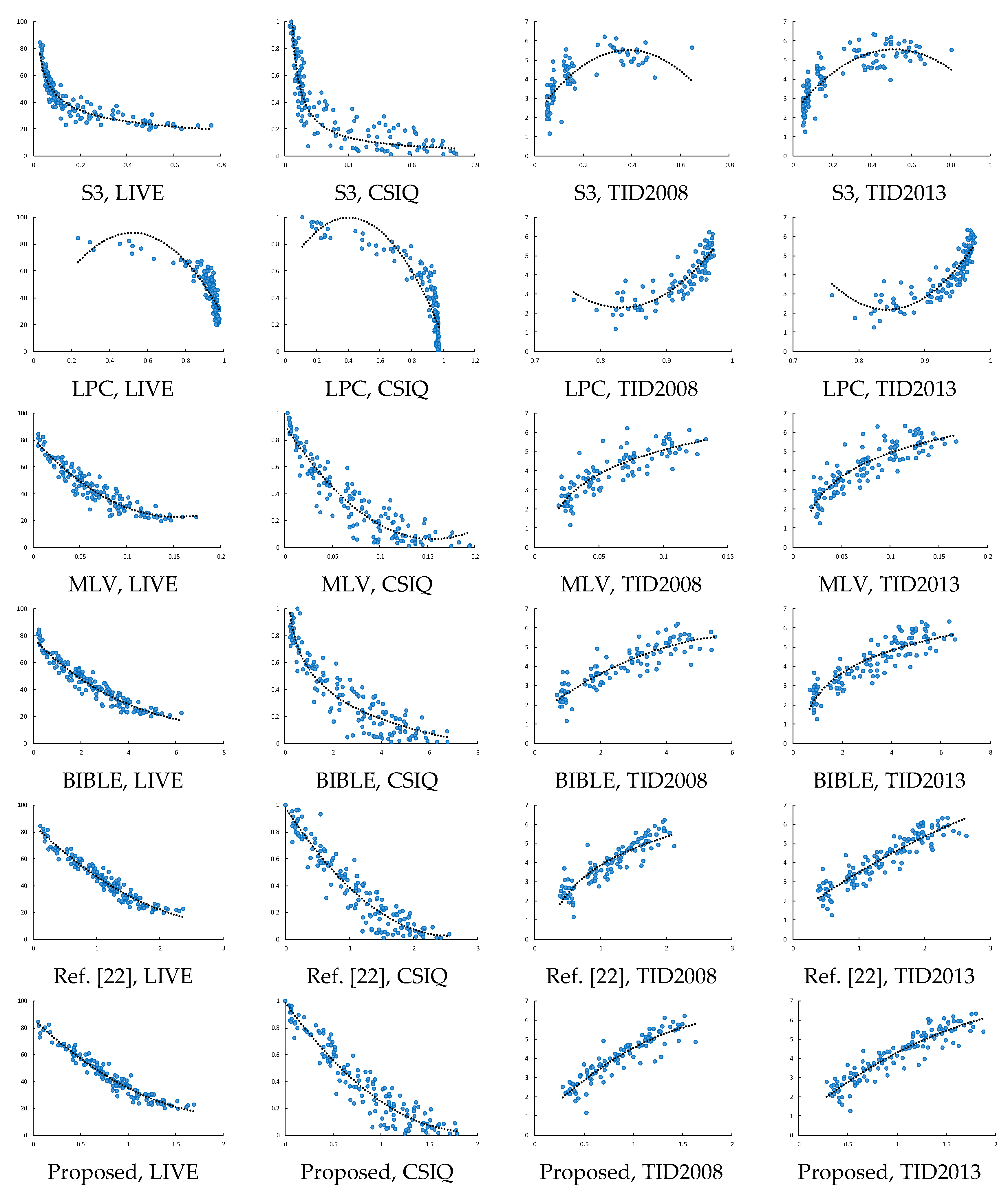
In order to illustrate the validity of the proposed method, we calculate the overall performance on the four public image databases. Figure 9 shows the scatter plots of the objective scores generated by the different methods versus the subjective scores given by the databases. We choose five recent methods for comparison, including S3, MLV, LPC, BIBLE, and Ref. [22].
In Figure 9, our method shows less biasness and the best correlation of all of the databases. LPC produces slightly worse results in the LIVE and CSIQ databases. In the other two databases, S3 produces slightly worse results. MLV, BIBLE, Ref. [22], and our method produce a somewhat similar fitting. Although, the fitting results produced by Ref. [22] are better than those of methods. A closer comparison indicates that our method achieves the best fitting results, because the scatter points are more densely and evenly clustered around the fitting line. For the four synthetic databases, our method achieves the best consistency and correlation.
We use four criteria to compare the performance of these methods, including PLCC, KRCC, SRCC, and RMSE. Some experimental results between the proposed method and the others on the four synthetic databases are summarized in Table 3. For each performance measure, we mark the top two results in boldface. Meanwhile, taking into account the differences between the number of images in the different databases, we calculate the weighted average value of the four synthetic databases. It is shown in Table 3 that our method demonstrates the best performance among all of the methods.
In order to verify our method, we use three criteria to compare the performance of six methods, including SRCC, PLCC, and RMSE. The experimental results are summarized in Table 4. In the CID2013 database, our method achieves the best accuracy and the second best monotonicity. In the BID database, our method achieves the second best accuracy and monotonicity. The experimental results indicated that our method also performs well on the real blur images.
3.2.3. Impact of Block Sizes
In the proposed method, the block size is crucial to the final blur score. In order to determine the block size, we set the block size from 4 × 4 to 12 × 12. For each block size, we calculate the average results of the SRCC, PLCC, and RMSE, which are listed in Table 5. It is shown in table that the best results can be achieved when the setting block size is 6 × 6. Therefore, the block size is selected 6 × 6 in the experiment.
4. Conclusions
Blur is one of the most critical factors that affects image quality. Hence, it is of great significance to design an objective assessment algorithm for the blur degree of the digital images. In this paper, we propose an efficient NR image blur assessment method. The three main contribution of our method are as follows: (1) we observed that to some extent the blur introduces distortion to the DCT coefficients, and thus we design a response function of the singular values (RFSV) to characterize the change; (2) we combine the spatial (i.e., variance of the blurred image) and spectral (i.e., DCT domain entropy of the gradient map) information to minimize the impact of the image content; and (3) we use SIFT-dependent weights to normalize the sum of RFSV, and therefore, the produced score is close to that assessed by the HVS. Compared with the six state-of-the-art NR methods on the six blurred image databases, the blur scores produced by our method are closest to the human subjective scores. Moreover, the proposed method achieves a high accuracy and strong robustness. While the existing methods are effective for synthetic blur, they are limited in predicting the real blur. Our method is more effective for the real blur than most of the existing methods, and yet there is still room for improvement. In the future, we will analyze more useful features and develop advanced assessment algorithms for the real blur databases.
Author Contributions
S.Z. designed the algorithm, P.L. conducted the experiments and wrote the paper, X.X. and L.L. analyzed the results, and C.-C.C. provided helpful suggestions.
Funding
This research was funded by the National Natural Science Foundation of China (Grant No.61370218), the Public Welfare Technology and Industry Project of Zhejiang Provincial Science Technology Department (Grant No. 2016C31081 and No. LGG18F020013) and the Key Research and Development Project of Zhejiang Province (Grant No. 2017C01022).
Conflicts of Interest
The authors declare no conflicts of interest.
References
- Wang, Z.; Bovik, A.C.; Sheikh, H.R.; Simoncelli, E.P. Image quality assessment: From error visibility to structural similarity. IEEE Trans. Image Process. 2004, 13, 600–612. [Google Scholar] [CrossRef] [PubMed]
- Sheikh, H.R.; Bovik, A.C.; De, V.G. An information fidelity criterion for image quality assessment using natural scene statistics. IEEE Trans. Image Process. 2005, 14, 2117–2128. [Google Scholar] [CrossRef] [PubMed] [Green Version]
- Sheikh, H.R.; Bovik, A.C. Image information and visual quality. IEEE Trans. Image Process. 2006, 15, 430–444. [Google Scholar] [CrossRef] [PubMed] [Green Version]
- Larson, E.C.; Chandler, D.M. Most apparent distortion: Full-reference image quality assessment and the role of strategy. J. Electron. Imaging 2010, 19, 011006. [Google Scholar]
- Zhang, L.; Zhang, L.; Mou, X.Q.; Zhang, D. FSIM: A feature similarity index for image quality assessment. IEEE Trans. Image Process. 2011, 20, 2378–2386. [Google Scholar] [CrossRef] [PubMed]
- Xue, W.F.; Zhang, L.; Mou, X.Q.; Bovik, A.C. Gradient magnitude similarity deviation: A highly efficient perceptual image quality index. IEEE Trans. Image Process. 2013, 23, 684–695. [Google Scholar] [CrossRef] [PubMed]
- Gao, X.; Lu, W.; Tao, D.; Li, X. Image quality assessment based on multiscale geometric analysis. IEEE Trans. Image Process. 2013, 18, 1409–1423. [Google Scholar]
- Tao, D.; Li, X.; Lu, W.; Gao, X. Reduced-reference IQA in contourlet domain. IEEE Trans. Syst. Man Cybern. Part B 2009, 39, 1623–1627. [Google Scholar]
- Soundararajan, R.; Bovik, A.C. RRED indices: Reduced reference entropic differencing for image quality assessment. IEEE Trans. Image Process. 2012, 21, 517–526. [Google Scholar] [CrossRef] [PubMed]
- Ma, L.; Li, S.N.; Zhang, F.; Ngan, K.N. Reduced-reference image quality assessment using reorganized DCT-based image representation. IEEE Trans. Multimed. 2011, 13, 824–829. [Google Scholar] [CrossRef]
- Wu, J.J.; Lin, W.S.; Shi, G.M.; Liu, A.M. Reduced-reference image quality assessment with visual information fidelity. IEEE Trans. Multimed. 2013, 15, 1700–1705. [Google Scholar] [CrossRef]
- Sun, T.; Ding, S.; Chen, W. Reduced-reference image quality assessment through SIFT intensity ratio. Int. J. Mach. Learn. Cybern. 2014, 5, 923–931. [Google Scholar] [CrossRef]
- Qi, F.; Zhao, D.B.; Gao, W. Reduced reference stereoscopic image quality assessment based on binocular perceptual information. IEEE Trans. Multimed. 2015, 17, 2338–2344. [Google Scholar] [CrossRef]
- Marziliano, P.; Dufaux, F.; Winkler, S.; Ebrahimi, T. Perceptual blur and ringing metrics: Application to JPEG2000. Signal Process. Image Commun. 2004, 19, 163–172. [Google Scholar] [CrossRef]
- Ferzli, R.; Karam, L.J. A no-reference objective image sharpness metric based on the notion of just noticeable blur (JNB). IEEE Trans. Image Process. 2009, 18, 717–728. [Google Scholar] [CrossRef] [PubMed]
- Narvekar, N.D.; Karam, L.J. A no-reference image blur metric based on the cumulative probability of blur detection (CPBD). IEEE Trans. Image Process. 2011, 18, 2678–2683. [Google Scholar] [CrossRef] [PubMed]
- Vu, C.T.; Phan, T.D.; Chandler, D.M. S3: A spectral and spatial measure of local perceived sharpness in natural images. IEEE Trans. Image Process. 2012, 21, 934–945. [Google Scholar] [CrossRef] [PubMed]
- Hassen, R.; Wang, Z.; Salama, M. Image sharpness assessment based on local phase coherence. IEEE Trans. Image Process. 2013, 22, 2798–2810. [Google Scholar] [CrossRef] [PubMed]
- Bahrami, K.; Kot, A.C. A fast approach for no-reference image sharpness assessment based on maximum local variation. IEEE Signal Process. Lett. 2014, 21, 751–755. [Google Scholar] [CrossRef]
- Kerouh, F.; Serir, A. Perceptual blur detection and assessment in the DCT domain. In Proceedings of the 4th International Conference on Electrical Engineering, Boumerdex, Algeria, 13–15 December 2015; pp. 1–4. [Google Scholar]
- Li, L.D.; Lin, W.S.; Wang, X.S.; Yang, G.B.; Bahrami, K.; Kot, A.C. No-reference image blur assessment based on discrete orthogonal moments. IEEE Trans. Cybern. 2016, 46, 39–50. [Google Scholar] [CrossRef] [PubMed]
- Zhang, S.Q.; Wu, T.; Xu, X.H.; Cheng, Z.M.; Pu, S.L.; Chang, C.C. No-reference image blur assessment based on SIFT and DCT. J. Inf. Hiding Multimed. Signal Process. 2018, 9, 219–231. [Google Scholar]
- Cai, H.; Li, L.D.; Qian, J.S. Image blur assessment with feature points. J. Inf. Hiding Multimed. Signal Process. 2015, 6, 2073–4212. [Google Scholar]
- Mukundan, R.; Ong, S.H.; Lee, P.A. Image analysis by Tchebichef moments. IEEE Trans. Image Process. 2001, 10, 1357–1364. [Google Scholar] [CrossRef] [PubMed]
- Zhang, L.; Gu, Z.Y.; Li, H.Y. SDSP: A novel saliency detection method by combining simple priors. In Proceedings of the 20th IEEE International Conference, Melbourne, Australia, 15–18 September 2013; pp. 171–175. [Google Scholar]
- Liu, L.; Liu, B.; Huang, H.; Bovik, A.C. No-reference image quality assessment based on spatial and spectral entropies. Signal Process. Image Commun. 2014, 29, 856–863. [Google Scholar] [CrossRef]
- Li, L.; Xia, W.; Lin, W.; Fang, Y.; Wang, S. No-reference and robust image sharpness evaluation based on multiscale spatial and spectral features. IEEE Trans. Multimed. 2017, 19, 1030–1040. [Google Scholar] [CrossRef]
- Sheikh, H.R.; Sabir, M.F.; Bovik, A.C. A statistical evaluation of recent full reference image quality assessment algorithms. IEEE Trans. Image Process. 2006, 15, 3440–3451. [Google Scholar] [CrossRef] [PubMed]
- Ponomarenko, N.; Lukin, V.; Zelensky, A.; Egiazarian, K.; Carli, M.; Battisti, F. TID2008—A database for evaluation of full reference visual quality assessment metrics. Adv. Mod. Radioelectron. 2009, 10, 30–45. [Google Scholar]
- Ponomarenko, N.; leremeiew, O.; Lukin, V.; Egiazarian, K.; Jin, L.; Astola, L. Color image database TID2013: Peculiarities and preliminary results. In Proceedings of the European Workshop on Visual Information Processing (EUVIP), Paris, France, 10–12 June 2013; pp. 106–111. [Google Scholar]
- Virtanen, T.; Nuutinen, M.; Vaahteranoksa, M.; Oittinen, P.; Hakkinen, J. CID2013: A database for evaluating no-reference image quality assessment algorithms. IEEE Trans. Image Process. 2015, 24, 390–402. [Google Scholar] [CrossRef] [PubMed]
- Ciancio, A.; Da, C.A.; Da, S.E.; Said, A.; Samadani, R.; Obrador, P. No-reference blur assessment of digital pictures based on multifeature classifiers. IEEE Trans. Image Process. 2011, 20, 64–75. [Google Scholar] [CrossRef] [PubMed]
- Lowe, D.G. Distinctive Image Features from scale-invariant keypoints. Int. J. Comput. Vis. 2004, 60, 91–110. [Google Scholar] [CrossRef]
Figure 1.
Flowchart of the proposed method. DCT—discrete cosine transform; RFSV—response function of singular values.
Figure 1.
Flowchart of the proposed method. DCT—discrete cosine transform; RFSV—response function of singular values.

Figure 2.
Distribution of the value of the difference matrix in the horizontal direction (x-axis) and vertical direction (y-axis) of a block with a different Gaussian blur: (a) ; (b) ; and (c) .
Figure 2.
Distribution of the value of the difference matrix in the horizontal direction (x-axis) and vertical direction (y-axis) of a block with a different Gaussian blur: (a) ; (b) ; and (c) .

Figure 3.
Distribution of singular values s1 (x-axis) against singular values s2 (y-axis) of thirty blocks with different standard deviations of the Gaussian blur: (a) ; (b) ; (c) ; and (d) .
Figure 3.
Distribution of singular values s1 (x-axis) against singular values s2 (y-axis) of thirty blocks with different standard deviations of the Gaussian blur: (a) ; (b) ; (c) ; and (d) .
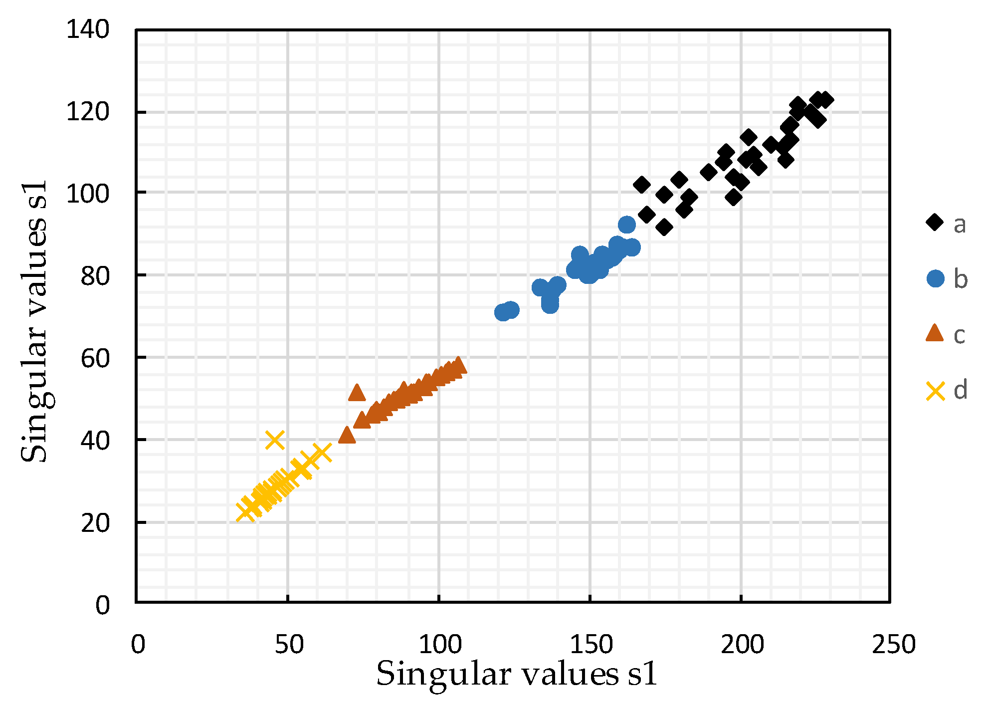
Figure 4.
Relationship between the sum of the RFSV and the Gaussian blur standard deviation. Each line represents an image of categorical subjective image quality [CSIQ] database.
Figure 4.
Relationship between the sum of the RFSV and the Gaussian blur standard deviation. Each line represents an image of categorical subjective image quality [CSIQ] database.

Figure 5.
Two images with the same entropy but different contents. (a) An image from categorical subjective image quality [CSIQ] database. (b) An image from categorical subjective image quality [CSIQ] database.
Figure 5.
Two images with the same entropy but different contents. (a) An image from categorical subjective image quality [CSIQ] database. (b) An image from categorical subjective image quality [CSIQ] database.

Figure 6.
(a) Blurred image and (b) saliency map.

Figure 7.
Six images with different blur degrees. DMOS—difference mean opinion score.

Figure 8.
Six images with similar blur degrees.

Figure 9.
Scatter plots of the objective scores generated by different methods versus subjective scores (DMOS for Video Engineering [LIVE] and categorical subjective image quality [CSIQ], mean opinion score [MOS] for Tampere Image Database 2008 [TID2008] and Tampere Image Database 2013 [TID2013]) on four image databases. The x-axis represents the objective score and the y-axis represents the subjective score.


Table 1.
Blur scores generated by different methods for the images in Figure 7. DMOS—difference mean opinion score; JNB—just noticeable blur; CPBD—cumulative probability of blur detection; S3—spectral and spatial sharpness; LPC—local phase coherence; MLV—maximum local variation; BIBLE—blind image blur evaluation.
| Image | (a) | (b) | (c) | (d) | (e) | (f) |
|---|---|---|---|---|---|---|
| DMOS | 0.0730 | 0.3000 | 0.5480 | 0.6730 | 0.7900 | 0.9630 |
| JNB [15] | 2.8646 | 1.5821 | 1.3920 | 1.2821 | 0.8128 | 1.1096 |
| CPBD [16] | 0.1210 | 0.1017 | 0.0033 | 0 | 0 | 0 |
| S3 [17] | 0.1107 | 0.1520 | 0.0637 | 0.0408 | 0.0597 | 0.0257 |
| LPC [18] | 0.9613 | 0.9474 | 0.8607 | 0.6935 | 0.5735 | 0.2031 |
| MLV [19] | 0.0721 | 0.0815 | 0.0239 | 0.0156 | 0.0119 | 0.0044 |
| BIBLE [21] | 3.5098 | 2.6294 | 1.2471 | 0.5666 | 0.2031 | 0.2689 |
| Ref. [22] | 1.4592 | 1.4238 | 0.6613 | 0.4199 | 0.1892 | 0.1638 |
| Ours | 0.9931 | 0.9439 | 0.4674 | 0.4415 | 0.2005 | 0.0669 |
Table 2.
Blur scores generated by different methods for the images in Figure 8.
Table 2.
Blur scores generated by different methods for the images in Figure 8.
| Image | (a) | (b) | (c) | (d) | (e) | (f) |
|---|---|---|---|---|---|---|
| DMOS | 29.9480 | 30.8705 | 31.0057 | 32.4380 | 34.9790 | 35.0583 |
| JNB [15] | 4.1472 | 3.5025 | 4.5699 | 5.1309 | 3.8593 | 4.1892 |
| CPBD [16] | 0.3273 | 0.5576 | 0.4599 | 0.5438 | 0.3902 | 0.3971 |
| S3 [17] | 0.1586 | 0.2394 | 0.2656 | 0.3621 | 0.1674 | 0.1252 |
| LPC [18] | 0.9571 | 0.9755 | 0.9592 | 0.9605 | 0.9543 | 0.9583 |
| MLV [19] | 0.0913 | 0.0939 | 0.0874 | 0.1035 | 0.0806 | 0.0666 |
| BIBLE [21] | 3.6730 | 3.8631 | 3.5880 | 3.9721 | 3.5388 | 3.3057 |
| Ref. [22] | 1.6156 | 1.6946 | 1.4822 | 1.4156 | 1.3212 | 1.2756 |
| Ours | 1.2174 | 1.1844 | 1.1146 | 1.0966 | 1.0117 | 0.9461 |
Table 3.
Comparison of our proposed method and six existing metrics on four synthetic databases. LIVE—Video Engineering; CSIQ—categorical subjective image quality; TID2008—Tampere Image Database 2008; TID2013—Tampere Image Database 2013; PLCC—Pearson Linear Correlation Coefficient; KRCC—Kendall rank order correlation coefficient; SRCC—Spearman Rank Order Correlation Coefficient; RMSE—root mean square error.
| Database | Criterion | CPBD | S3 | LPC | MLV | BIBLE | Ref. [22] | Ours |
|---|---|---|---|---|---|---|---|---|
| LIVE | PLCC | 0.8956 | 0.9436 | 0.9017 | 0.9429 | 0.9622 | 0.9694 | 0.9739 |
| KRCC | 0.7652 | 0.8004 | 0.7149 | 0.7776 | 0.8328 | 0.8464 | 0.8561 | |
| SRCC | 0.9190 | 0.9441 | 0.8886 | 0.9316 | 0.9611 | 0.9671 | 0.9712 | |
| RMSE | 6.9929 | 5.2058 | 6.7972 | 5.2366 | 4.2815 | 3.8603 | 3.5713 | |
| CSIQ | PLCC | 0.8818 | 0.9107 | 0.9412 | 0.9488 | 0.9403 | 0.9492 | 0.9518 |
| KRCC | 0.7079 | 0.7294 | 0.7683 | 0.7713 | 0.7439 | 0.7678 | 0.7688 | |
| SRCC | 0.8847 | 0.9059 | 0.9224 | 0.9247 | 0.9132 | 0.9272 | 0.9294 | |
| RMSE | 0.1351 | 0.1184 | 0.0968 | 0.0905 | 0.0975 | 0.0902 | 0.0879 | |
| TID2008 | PLCC | 0.8235 | 0.8541 | 0.8903 | 0.8585 | 0.8929 | 0.9101 | 0.9151 |
| KRCC | 0.6310 | 0.6124 | 0.7155 | 0.6524 | 0.7009 | 0.7381 | 0.7640 | |
| SRCC | 0.8412 | 0.8418 | 0.8959 | 0.8548 | 0.8915 | 0.9075 | 0.9239 | |
| RMSE | 0.6657 | 0.6104 | 0.5344 | 0.6018 | 0.5284 | 0.4862 | 0.4731 | |
| TID2013 | PLCC | 0.8552 | 0.8813 | 0.8197 | 0.8827 | 0.9051 | 0.9264 | 0.9276 |
| KRCC | 0.6467 | 0.6397 | 0.7479 | 0.6810 | 0.7066 | 0.7479 | 0.7660 | |
| SRCC | 0.8518 | 0.8609 | 0.9191 | 0.8787 | 0.8988 | 0.9243 | 0.9327 | |
| RMSE | 0.6467 | 0.5896 | 0.7148 | 0.5865 | 0.5305 | 0.4699 | 0.4660 | |
| Weighted average | PLCC | 0.8680 | 0.9019 | 0.8912 | 0.9139 | 0.9288 | 0.9418 | 0.9451 |
| KRCC | 0.6944 | 0.7051 | 0.7384 | 0.7285 | 0.7515 | 0.7792 | 0.7915 | |
| SRCC | 0.8780 | 0.8943 | 0.9071 | 0.9021 | 0.9189 | 0.9350 | 0.9396 | |
| RMSE | 2.2724 | 1.7449 | 2.1976 | 1.7430 | 1.4509 | 1.3087 | 1.2240 |
Table 4.
Comparison of our proposed method and six existing metrics on two real blur databases. BID—Blurred Image Database; CID2013—Camera Image Database.
Table 4.
Comparison of our proposed method and six existing metrics on two real blur databases. BID—Blurred Image Database; CID2013—Camera Image Database.
| Database | Criterion | CPBD | S3 | LPC | MLV | BIBLE | Ref. [22] | OURS |
|---|---|---|---|---|---|---|---|---|
| CID2013 | PLCC | 0.5254 | 0.6863 | 0.7013 | 0.6890 | 0.6943 | 0.6770 | 0.7104 |
| SRCC | 0.4448 | 0.6460 | 0.6024 | 0.6206 | 0.6888 | 0.6685 | 0.6843 | |
| RMSE | 19.4530 | 16.6190 | 16.2474 | 16.5594 | 16.4794 | 16.8530 | 16.1160 | |
| BID | PLCC | 0.2704 | 0.4271 | 0.3901 | 0.3643 | 0.3606 | 0.3018 | 0.3915 |
| SRCC | 0.2717 | 0.4253 | 0.3161 | 0.3236 | 0.3165 | 0.2935 | 0.3352 | |
| RMSE | 1.2053 | 0.1320 | 1.1528 | 1.1659 | 1.1876 | 1.1935 | 1.1506 |
Table 5.
Average values of three criteria for different block sizes.
| Size | 4 × 4 | 6 × 6 | 8 × 8 | 10 × 10 | 12 × 12 |
|---|---|---|---|---|---|
| PLCC | 0.9191 | 0.9451 | 0.9407 | 0.9423 | 0.9408 |
| SRCC | 0.9100 | 0.9396 | 0.9335 | 0.9341 | 0.9319 |
| RMSE | 1.5724 | 1.2240 | 1.2279 | 1.2378 | 1.3086 |
© 2018 by the authors. Licensee MDPI, Basel, Switzerland. This article is an open access article distributed under the terms and conditions of the Creative Commons Attribution (CC BY) license (http://creativecommons.org/licenses/by/4.0/).
Share and Cite
MDPI and ACS Style
Zhang, S.; Li, P.; Xu, X.; Li, L.; Chang, C.-C. No-Reference Image Blur Assessment Based on Response Function of Singular Values. Symmetry 2018, 10, 304. https://doi.org/10.3390/sym10080304
AMA Style
Zhang S, Li P, Xu X, Li L, Chang C-C. No-Reference Image Blur Assessment Based on Response Function of Singular Values. Symmetry. 2018; 10(8):304. https://doi.org/10.3390/sym10080304
Chicago/Turabian StyleZhang, Shanqing, Pengcheng Li, Xianghua Xu, Li Li, and Ching-Chun Chang. 2018. "No-Reference Image Blur Assessment Based on Response Function of Singular Values" Symmetry 10, no. 8: 304. https://doi.org/10.3390/sym10080304
Note that from the first issue of 2016, this journal uses article numbers instead of page numbers. See further details here.