A Forecasting Model Based on Multi-Valued Neutrosophic Sets and Two-Factor, Third-Order Fuzzy Fluctuation Logical Relationships


1
School of Management Science and Engineering, Shandong University of Finance and Economics, Jinan 250014, China
2
School of Management, Jiangsu University, Zhenjiang 212013, China
3
Rensselaer Polytechnic Institute, Troy, NY 12180, USA
*
Author to whom correspondence should be addressed.
Symmetry 2018, 10(7), 245; https://doi.org/10.3390/sym10070245
Submission received: 29 May 2018
/
Revised: 17 June 2018
/
Accepted: 25 June 2018
/
Published: 28 June 2018
(This article belongs to the Special Issue Algebraic Structures of Neutrosophic Triplets, Neutrosophic Duplets, or Neutrosophic Multisets)
Abstract
:Making predictions according to historical values has long been regarded as common practice by many researchers. However, forecasting solely based on historical values could lead to inevitable over-complexity and uncertainty due to the uncertainties inside, and the random influence outside, of the data. Consequently, finding the inherent rules and patterns of a time series by eliminating disturbances without losing important details has long been a research hotspot. In this paper, we propose a novel forecasting model based on multi-valued neutrosophic sets to find fluctuation rules and patterns of a time series. The contributions of the proposed model are: (1) using a multi-valued neutrosophic set (MVNS) to describe the fluctuation patterns of a time series, the model could represent the fluctuation trend of up, equal, and down with degrees of truth, indeterminacy, and falsity which significantly preserve details of the historical values; (2) measuring the similarities of different fluctuation patterns by the Hamming distance could avoid the confusion caused by incomplete information from limited samples; and (3) introducing another related time series as a secondary factor to avoid warp and deviation in inferring inherent rules of historical values, which could lead to more comprehensive rules for further forecasting. To evaluate the performance of the model, we explored the Taiwan Stock Exchange Capitalization Weighted Stock Index (TAIEX) as the major factor we forecast, and the Dow Jones Index as the secondary factor to facilitate the predicting of the TAIEX. To show the universality of the model, we applied the proposed model to forecast the Shanghai Stock Exchange Composite Index (SHSECI) as well.
1. Introduction
Financial forecasting problems are one of the most complex problems in the modern economic environment. It is well known that there is a statistical long-range dependency between the current values and historical values in different times of certain time series [1]. With this understanding, as well as the development of statistics and probability, former researchers designed exponential smoothing (ES), autoregressive and moving average (ARMA), autoregressive integrated moving average (ARIMA), and seasonal ARIMA to forecast time series [2,3]. However, because the historical values contain considerable amounts of noise and randomness, a model solely based on real historical values could not fully convey the inherent rules.
To find the general rules of time series, Song and Chissom [4] introduced fuzzy set theory into time series and proposed the concepts of fuzzy time series (FTS). They used historical data and max-min composition operations to establish a fuzzy time series model to predict the enrollment at the University of Alabama [5]. To conceive a more general and representative method of prediction, a vast number of fuzzy time series models combined with autoregressive (AR) models and moving average (MA) models [6,7] based on fuzzy lagged variables of time series were proposed which helped the refinement of prediction with large degree. Those models can successfully convey the general rules of the time series; however, the composition operation is complicated and sometimes the designed algorithms could not fully represent the inherent problems. Later, Chen [8] improved the model by using simplified arithmetic operations. After that, the model is extended to a high-order FTS model to reflect more details of history to improve the prediction performance of university enrollment [9]. On this basis, more researchers proposed novel models by combining high-order FTS with other algorithms to improve the performance. For example, Chen and Chung [10] combined genetic algorithms with fuzzy time series. Aladag et al. [11] and Chen [12] presented a high-order fuzzy time series forecasting model based on adaptive expectations and artificial neural networks, etc. Zhang et al. [13,14] proposed a visibility graph prediction model with the revision of fuzzy logic to improve the precision of the forecasting result. These models always need other facilitating methods to help with the improvement in accuracy.
In fact, the fluctuations of different stock markets have a certain correlation. Therefore, some researchers began to introduce other time series into their forecasting model to improve their forecasting performance. For example, Chen and Hwang [15] presented a two-factor fuzzy time series forecasting model. Later, Lee et al. [16] and Guan et al. [17] presented a two-factor high-order fuzzy time series model. Wang and Chen [18] presented a comprehensive method based on automatic clustering techniques and two-factor high-order fuzzy time series. Singh et al. [19] proposed a model based on two-factor high-order fuzzy time series and artificial neural networks, etc. Obviously, the consideration of other time series improved the performance of the traditional forecasting model. However, more datasets involved more complex and inconsistent information to be described. Thus, some new theories are needed to express the information in this context.
With the increasing need to depict imprecise and inconsistent information, intuitionistic fuzzy set (IFS) [6] theory is among the effective extensions of fuzzy set theory to deal with the vagueness and randomness within the data. To solve the decision-making problems even more effectively and successfully, Smarandache [20] proposed neutrosophic sets (NSs) from the philosophical thinking which consisted of three degrees of truth, indeterminacy, and falsity. Up to this point, the various extensions of NSs have been studied by many researchers to solve multi-criteria decision-making (MCDM) problems [21,22,23,24,25,26,27,28,29,30,31,32,33,34,35,36,37,38]. For example, Wang et al. [21,22] and Garg [32] defined single-valued neutrosophic sets (SVNSs) and interval neutrosophic sets (INSs) which are characterized by three real numbers and intervals, respectively. Ye [23] proposed the similarity measures between INSs which are used between each alternative and the ideal alternative to rank the alternatives. Garg [33] also proposed a linguistic single-valued neutrosophic set (LSVNS) to present a decision-making approach. Researchers also found SVNS theory could incorporate with measure theory and be adopted in many real-life situations with great randomness and uncertainty, such as pattern recognition and medical diagnosis by entropy measures [29], similarity measures [34,35,36] and biparametric distance measures [37]. However, due to the ambiguity and intricacy of some real-life situations, the truth-membership degree, indeterminacy-membership degree, and falsity membership degree may be represented by several possible values. These above extensions cannot properly solve the problems. Under these circumstances, Wang [25] introduced multi-valued neutrosophic sets (MVNSs) to express the information and improve the operations and comparison methods of MVNSs. MVNSs are characterized by truth-membership, indeterminacy-membership, and false-membership functions that have a set of crisp values in the range [0, 1]. In recent years, MVNSs have been applied to complex practical problems. For example, Ji [28] applied MVNSs to describe information on personnel selection. Furthermore, some scholars have applied SVNSs to the financial field to solve the problem of stock market prediction [38]. With the consideration of the complexity and uncertainty in the financial field, in this paper, we explore the utility of MVNSs in our proposed method.
In this paper, we propose a novel forecasting model based on MVNSs and two-factor third-order fuzzy logical relationships to forecast the stock market. The major contributions are: (1) using a MVNS to describe the fluctuation pattern of time series, the model could represent the fluctuation of up, equal, and down with degrees of truth, indeterminacy, and falsity introduced by the MVNS, which significantly preserved details of the historical values; (2) measuring the similarities of different fluctuation patterns of different time series by the Hamming distance could avoid the confusion caused by incomplete information from samples; and (3) due to the existence of likeness among similar types of historical values, in this model, we introduce another related time series as a secondary factor to avoid warp and deviation in inferring inherent rules of historical values, which could lead to more comprehensive rules for further forecasting. To illustrate the steps, first, we convert the historical training data of the main factor and the secondary factor, respectively, from the original time series to fluctuation time series by comparing with each data and that of the previous day. Then, we fuzzify the historical training data to form two-factor third-order fuzzy logical relationships based on MVNSs. Next, MVNSs, which represent the two-factor fuzzy logical relationships, can show the possibility of three trends. Finally, the Hamming distance measurement is used to find the most suitable logical rules to predict its future through the previously obtained multi-valued neutrosophic logical relationship and historical data.
The remainder of this paper is organized as follows: in the next section, we review and define some concepts of fuzzy-fluctuation time series and MVNSs. In the third section, a novel approach for forecasting is described based on MVNS theory and hamming distance. In the fourth section, the experimental results of the proposed method are compared with the existing methods and we also use the proposed model to forecast the Taiwan Stock Exchange Capitalization Weighted Stock Index (TAIEX) from 1998 to 2006 and the Shanghai Stock Exchange Composite Index (SHSECI) from 2004 to 2015. The conclusions are discussed in Section 5.
2. Preliminaries
In this part, the general definitions of a fuzzy fluctuation time series in the model based on MVNSs are outlined.
Definition 1.
Letbe a linguistic set in the universe of discourse; it can be defined by its membership function,[0,1], wheredenotes the grade of membership of,.
The fluctuation trends of a stock market can be expressed by a linguistic set = {down, slightly down, equal, slightly up, up}. The element and its subscript i is strictly monotonically increasing [28], so the function can be defined as follows: .
Definition 2.
Letbe a time series of real numbers, where T is the number of the time series. is defined as a fluctuation time series, where. Each element ofcan be represented by a fuzzy setas defined in Definition 1. Then we call time seriesto be fuzzified into a fuzzy-fluctuation time series (FFTS).
Definition 3.
Let S(t) (t = n + 1, n + 2, …, T, n ≥ 1) be a FFTS. If S(t) is determined by, then the fuzzy-fluctuation logical relationship is represented by:
In the same way, let S(t) (t = n + 1, n + 2, …, T, n ≥ 1) be a two-factor FFTS. If the next status of S(t) is caused by the current status of and, the two-factor nth-order fuzzy-fluctuation is represented by:
and it is called the two-factor nth-order fuzzy-fluctuation logical relationship (FFLR) of the fuzzy-fluctuation time series, whereis called the left-hand side (LHS) andis called the right-hand side (RHS) of the FFLR, and.
Definition 4.
Let X be a space of objects with a generic element in X denoted by x. A neutrosophic set A in X is characterized by a truth-membership function, an indeterminacy-membership function, and a falsity-membership function. If a neutrosophic set A consists of, they can be defined by their membership function, whileare subsets of [0, 1], and A can be represented by [18]:
Definition 5.
Letbe the truth-membership, indeterminacy-membership and falsity-membership of a neutrosophic set A(t), respectively. The LHS of an nth-order FFLRcan be generated by:
whereif S(t − j) = i and 0, otherwise,represents the corresponding relationship between elementand the kth membership of a neutrosophic set A(t). Thus, the LHS of a nth-order FFLRcan be converted into a neutrosophic set.
Definition 6.
For S(t) (t = n + 1, n + 2, …, T, n ≥ 1) be a FFTS and A(t) be the LHS of a multi-valued neutrosophic logical relationship (MNLR), the FFLRs with the corresponding A(t) can be grouped into a fuzzy-fluctuation logical relationship group (FFLRG) by putting all their RHSs together as on the RHS of the FFLRG. Then, count the RHSs according to their linguistic values. The RHS of the FFLRG can also be converted into a neutrosophic set according to Definition 5.
For example, there is a FFLR , the corresponding FFLRG are , and the corresponding relationship between a linguistic set and a neutrosophic set are (1,0,0), (0.5,0.5,0), (0,1,0), (0,0.5,0.5), (0,0,1), respectively. Then the FFLRG can be converted to a MNLR .
Definition 7.
In this way, let A = {(0.5,0.6), (0.4,0.4), (0.2,0.2)} and B = {(0.5,0.5), (0.5,0.5), (0.1,0.3)} be two MVNSs. Then the following can be true:
Definition 8.
Letbe, respectively, MVNSs, so the expected value of A can be defined by [19]:
whererespectively represent the number of elements in.
3. A Novel Forecasting Model Based on Multi-Valued Neutrosophic Logical Relationships
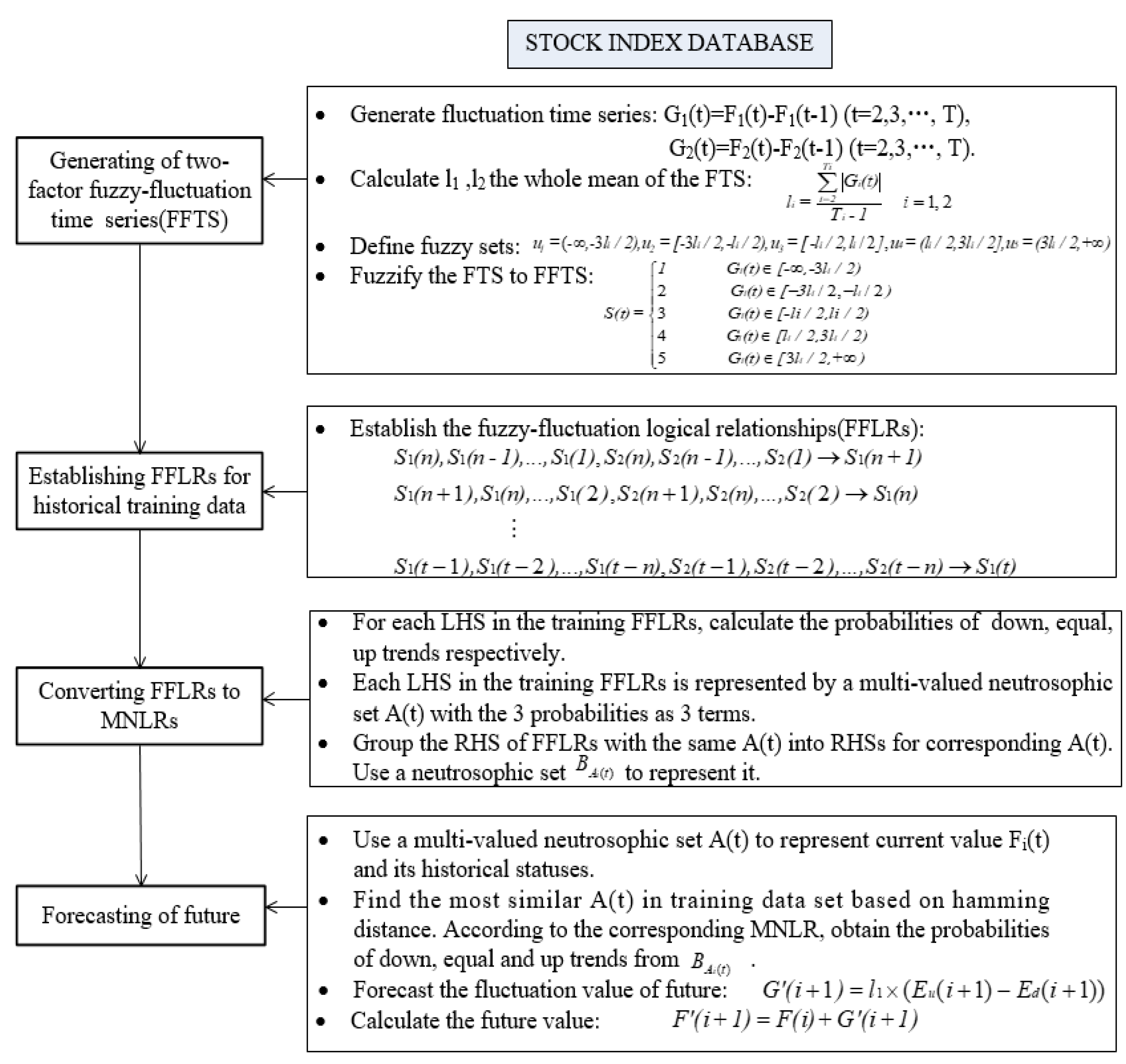
In this section, we present a novel fuzzy forecasting method based on multi-valued neutrosophic logical relationships and the Hamming distance. The data from January to October in one year are used as the training time series and the data from November to December are used as the testing dataset. The proposed model is now presented as follows and the basic steps of that areshown in Figure 1.
Step 1: Construct FFTS from the training data of two historical factors. For each element in the historical time series of the two factors, its fluctuation trend is defined by . which can be fuzzified into a linguistic set {down, equal, up} depending on its range and orientation of the fluctuations. Thus, in the same way, we can also divide it into five ranges, such as {down, slightly down, equal, slightly up, up}, , similarly, can also be divided into five parts, and are, respectively, defined as the whole mean of all elements in the fluctuation time series and .
Step 2: Determine the two-factor fuzzy fluctuation time series according to Definition 3. Each can be represented by its previous n days’ fuzzy fluctuation numbers, which can be used to establish nth-order FFLRs.
Step 3: According to Definition 4 and Definition 5, we use the MVNS A(t) to express the LHS of each FFLR. Each defined in step 1 represents a different magnitude of increase or decrease, so the MVNSs can be obtained by assigning weights to different states. Then, we can generate the RHSs for different LHSs, respectively, which are described in Definition 6. Thus, FFLRs of the historical training dataset can convert to MNLRs.
The nth-order fuzzy-fluctuation trends of each point in the test dataset can be represented by a MVNS . For each , compare with , respectively, and find the most similar one by using the Hamming distance method described in Definition 7.
Step 4: Choose the corresponding as the forecasting rule to forecast the fluctuation value of the next point according to Definition 8. Finally, obtain the forecasting value by .
4. Empirical Analysis
4.1. Forecasting the Taiwan Stock Exchange Capitalization Weighted Stock Index
In this section, we take TAIEX2004 as an example to illustrate the process of forecasting the TAIEX with the proposed method. The TAIEX2004 and the Dow Jones from January to October are respectively used as the training time series of two factors and the data from November to December are used as the testing dataset [39,40].
Step 1: First, we used the historical training data in TAIEX2004 and Dow Jones2004 to calculate the fluctuation trend. The whole mean of the fluctuation numbers of the two training datasets can be calculated to define the intervals. Then, the fluctuation time series of the two factors can be converted into FFTS, respectively. For example, the whole means of the historical dataset of TAIEX2004 and Dow Jones from January to October are 67 and 54. That is to say, = 67 and = 54. For example, = 6041.56 and = 6125.42, = − = 83.86, = 4, and = 10,409.85, = 10,544.07, = = 134.22, = 5. In this way, the two-factor fuzzified fluctuation dataset can be shown in the Appendix A
(Table A1 and Table A2, respectively).
Step 2: Considering the impact of the previous three days’ historical data on future forecasting, we choose the previous three days to establish FFLRs. The third-order FFLRs for the two-factor fuzzy fluctuation time series forecasting model are established based on the FFTS from 2 January 2004 to 30 October 2004, as shown in Table A1 and Table A2.
Step 3: To convert the LHSs of the FFLRs in Table A1 and Table A2 to MVNSs. Due to the different degree of expression for each , we assumed that the each pre-defined in step 1 corresponds to the different neutrosophic sets, such as {0, 0, 1}, {0, 0.5, 0.5}, {0, 1, 0}, {0.5, 0.5, 0}, and {1, 0, 0}. Then, we group the RHSs of the FFLRs and convert the FFLR to MNLR according to Definitions 5–7. For example, the LHS of FFLR 2,4,4→4 and 2,4,3→3 can be represented by a MVNS {(0.33,0.17), (0.5,0.67), (0.17,0.17)}. Then, the Hamming distance can be used to obtain the most suitable MVNSs. The detailed grouping and converting processes are shown in Figure 2.
In this way, the FFLR 2,4,4→4 and 2,4,3→3 is converted into a MNLR {(0.33,0.17), (0.5,0.67), (0.17,0.17)}→(0.25,0.41,0.33). Therefore, the FFLRs of test dataset can be converted into MNLRs, as shown in Table A3.
Step 4: Based on the MNLRs obtained in Step 3, we forecast the test dataset from 1 November to 31 December 2004. For example, from Table 1 the forecasting value of the TAIEX on 1 November 2004 is calculated as follows.
The MVNSs on 1 November 2004 is {(0.17,0.33), (0.83,0.67), (0,0)}, then we can find the best rule {(0.17,0.33), (0.83,0.67), (0,0)}→(0,1,0) to forecast its future according to Table A3. Respectively, we calculate the expected number of the MNLR according to Definition 8, the expected value:
The fluctuation from current value to next value can be obtained for forecasting by defuzzifying the fluctuation fuzzy number, shown as follows:
Finally, the forecasted value can be obtained by the current value and the fluctuation value:
To confirm the performance of the proposed method, we compare the difference between the forecasted values and the actual values. The performance can be evaluated using the mean squared error (MSE), root of the mean squared error (RMSE), mean absolute error (MAE), mean percentage error (MPE), etc. These indicators are defined by Equations (8)–(11):
where n denotes the number of values to be forecasted, and forecast(t) and actual(t) denote the predicted value and actual value at time t, respectively. From Table 1, we can calculate the MSE, RMSE, MAE, and MPE are 2809.94, 53.01, 38.58, and 0.0066, respectively.
Let the order of n be 1, 3, 5, 7, 9, from Table 2; we can see that third-order forecasting model is relatively accurate compared to the others.
To prove the validity of the proposed method, the TAIEX from 1998 to 2006 is employed to forecast in the same way. The forecasting results and errors are shown in Figure 4 and Table 3.
In Table 4, we can verify the model availability by comparing with the RMSEs of different methods for forecasting the TAIEX2004. The advantages of the proposed method are that it does not need to determine the boundary of discourse and the interaction of two factors. The method proposed is simple and suitable for practical application.
4.2. Forecasting the Shanghai Stock Exchange Composite Index
We applied the method to forecast SHSECI, which occupies an important position in China [48]. The Dow Jones was chosen as a secondary factor to build the model. For each year, we used the data from January to October to be the training data, and then we forecast SHSECI from November to December. The RMSE of forecast errors are shown in Table 5.
As is shown in Table 5, forecasting the SHSECI stock market obtains great results by using the proposed method.
5. Conclusions
In this paper, we propose a novel forecasting model for financial forecasting problems based on multi-valued neutrosophic logical relationships and Hamming distance. The major contributions are the usage of a multi-valued neutrosophic set (MVNS). Due to its ability in reflecting the up, equal, and down fluctuation trends, it can efficiently represent the inherent rules of the stock market. Meanwhile, Hamming distances of different MVNS could measure the similarity between different fluctuation patterns. We also applied another related time series as a secondary factor to help with qualifying the prediction of the main stock market. The empirical analysis showed that our model could perform well in forecasting different stock markets in different years. In fact, there are many other factors inside the stock market which can influence the fluctuation patterns. For example, volume fluctuation may also be considered as another facilitating factor. We would also consider applying the model in forecasting other time series, such as university enrollment, power consumption, etc.
Author Contributions
Project Administration, H.G.; Writing-Original Draft Preparation, J.H.; Software, Z.D.; Supervision, A.Z.; Writing-Review & Editing, S.G.
Funding
This work was supported by the National Natural Science Foundation of China under grant 71471076, the Fund of the Ministry of Education of Humanities and Social Sciences (14YJAZH025), the Fund of the China Nation Tourism Administration (15TACK003), the Natural Science Foundation of Shandong Province (ZR2013GM003), and the Foundation Program of Jiangsu University (16JDG005).
Acknowledgments
The authors are indebted to anonymous reviewers for their very insightful comments and constructive suggestions, which help ameliorate the quality of this paper.
Conflicts of Interest
The authors declare no conflict of interest.
Appendix A

Table A1.
Historical training data and fuzzified fluctuation data of Taiwan Stock Exchange Capitalization Weighted Stock (TAIEX) 2004.
Table A1.
Historical training data and fuzzified fluctuation data of Taiwan Stock Exchange Capitalization Weighted Stock (TAIEX) 2004.
| Date (YYYY/MM/DD) | TAIEX | Fluctuation | Fuzzified | Date (YYYY/MM/DD) | TAIEX | Fluctuation | Fuzzified | Date (YYYY/MM/DD) | TAIEX | Fluctuation | Fuzzified |
|---|---|---|---|---|---|---|---|---|---|---|---|
| 2004/1/2 | 6041.56 | - | - | 2004/4/16 | 6818.2 | 81.41 | 4 | 2004/7/23 | 5373.85 | -14.11 | 3 |
| 2004/1/5 | 6125.42 | 83.86 | 4 | 2004/4/19 | 6779.18 | −39.02 | 2 | 2004/7/26 | 5331.71 | −42.14 | 2 |
| 2004/1/6 | 6144.01 | 18.59 | 3 | 2004/4/20 | 6799.97 | 20.79 | 3 | 2004/7/27 | 5398.61 | 66.9 | 4 |
| 2004/1/7 | 6141.25 | −2.76 | 3 | 2004/4/21 | 6810.25 | 10.28 | 3 | 2004/7/28 | 5383.57 | −15.04 | 3 |
| 2004/1/8 | 6169.17 | 27.92 | 3 | 2004/4/22 | 6732.09 | −78.16 | 2 | 2004/7/29 | 5349.66 | −33.91 | 2 |
| 2004/1/9 | 6226.98 | 57.81 | 4 | 2004/4/23 | 6748.1 | 16.01 | 3 | 2004/7/30 | 5420.57 | 70.91 | 4 |
| 2004/1/12 | 6219.71 | −7.27 | 3 | 2004/4/26 | 6710.7 | −37.4 | 2 | 2004/8/2 | 5350.4 | −70.17 | 2 |
| 2004/1/13 | 6210.22 | −9.49 | 3 | 2004/4/27 | 6646.8 | −63.9 | 2 | 2004/8/3 | 5367.22 | 16.82 | 3 |
| 2004/1/14 | 6274.97 | 64.75 | 4 | 2004/4/28 | 6574.75 | −72.05 | 2 | 2004/8/4 | 5316.87 | −50.35 | 2 |
| 2004/1/15 | 6264.37 | −10.6 | 3 | 2004/4/29 | 6402.21 | −172.54 | 1 | 2004/8/5 | 5427.61 | 110.74 | 5 |
| 2004/1/16 | 6269.71 | 5.34 | 3 | 2004/4/30 | 6117.81 | −284.4 | 1 | 2004/8/6 | 5399.16 | −28.45 | 3 |
| 2004/1/27 | 6384.63 | 114.92 | 5 | 2004/5/3 | 6029.77 | −88.04 | 2 | 2004/8/9 | 5399.45 | 0.29 | 3 |
| 2004/1/28 | 6386.25 | 1.62 | 3 | 2004/5/4 | 6188.15 | 158.38 | 5 | 2004/8/10 | 5393.73 | −5.72 | 3 |
| 2004/1/29 | 6312.65 | −73.6 | 2 | 2004/5/5 | 5854.23 | −333.92 | 1 | 2004/8/11 | 5367.34 | −26.39 | 3 |
| 2004/1/30 | 6375.38 | 62.73 | 4 | 2004/5/6 | 5909.79 | 55.56 | 4 | 2004/8/12 | 5368.02 | 0.68 | 3 |
| 2004/2/2 | 6319.96 | −55.42 | 2 | 2004/5/7 | 6040.26 | 130.47 | 5 | 2004/8/13 | 5389.93 | 21.91 | 3 |
| 2004/2/3 | 6252.23 | −67.73 | 2 | 2004/5/10 | 5825.05 | −215.21 | 1 | 2004/8/16 | 5352.01 | −37.92 | 2 |
| 2004/2/4 | 6241.39 | −10.84 | 3 | 2004/5/11 | 5886.36 | 61.31 | 4 | 2004/8/17 | 5342.49 | −9.52 | 3 |
| 2004/2/5 | 6268.14 | 26.75 | 3 | 2004/5/12 | 5958.79 | 72.43 | 4 | 2004/8/18 | 5427.75 | 85.26 | 4 |
| 2004/2/6 | 6353.35 | 85.21 | 4 | 2004/5/13 | 5918.09 | −40.7 | 2 | 2004/8/19 | 5602.99 | 175.24 | 5 |
| 2004/2/9 | 6463.09 | 109.74 | 5 | 2004/5/14 | 5777.32 | -140.77 | 1 | 2004/8/20 | 5622.86 | 19.87 | 3 |
| 2004/2/10 | 6488.34 | 25.25 | 3 | 2004/5/17 | 5482.96 | -294.36 | 1 | 2004/8/23 | 5660.97 | 38.11 | 4 |
| 2004/2/11 | 6454.39 | −33.95 | 2 | 2004/5/18 | 5557.68 | 74.72 | 4 | 2004/8/26 | 5813.39 | 152.42 | 5 |
| 2004/2/12 | 6436.95 | −17.44 | 3 | 2004/5/19 | 5860.58 | 302.9 | 5 | 2004/8/27 | 5797.71 | −15.68 | 3 |
| 2004/2/13 | 6549.18 | 112.23 | 5 | 2004/5/20 | 5815.33 | −45.25 | 2 | 2004/8/30 | 5788.94 | −8.77 | 3 |
| 2004/2/16 | 6565.37 | 16.19 | 3 | 2004/5/21 | 5964.94 | 149.61 | 5 | 2004/8/31 | 5765.54 | −23.4 | 3 |
| 2004/2/17 | 6600.47 | 35.1 | 4 | 2004/5/24 | 5942.08 | −22.86 | 3 | 2004/9/1 | 5858.14 | 92.6 | 4 |
| 2004/2/18 | 6605.85 | 5.38 | 3 | 2004/5/25 | 5958.38 | 16.3 | 3 | 2004/9/2 | 5852.85 | −5.29 | 3 |
| 2004/2/19 | 6681.52 | 75.67 | 4 | 2004/5/26 | 6027.27 | 68.89 | 4 | 2004/9/3 | 5761.14 | −91.71 | 2 |
| 2004/2/20 | 6665.54 | −15.98 | 3 | 2004/5/27 | 6033.05 | 5.78 | 3 | 2004/9/6 | 5775.99 | 14.85 | 3 |
| 2004/2/23 | 6665.89 | 0.35 | 3 | 2004/5/28 | 6137.26 | 104.21 | 5 | 2004/9/7 | 5846.83 | 70.84 | 4 |
| 2004/2/24 | 6589.23 | −76.66 | 2 | 2004/5/31 | 5977.84 | −159.42 | 1 | 2004/9/8 | 5846.02 | −0.81 | 3 |
| 2004/2/25 | 6644.28 | 55.05 | 4 | 2004/6/1 | 5986.2 | 8.36 | 3 | 2004/9/9 | 5842.93 | −3.09 | 3 |
| 2004/2/26 | 6693.25 | 48.97 | 4 | 2004/6/2 | 5875.67 | −110.53 | 1 | 2004/9/10 | 5846.19 | 3.26 | 3 |
| 2004/2/27 | 6750.54 | 57.29 | 4 | 2004/6/3 | 5671.45 | −204.22 | 1 | 2004/9/13 | 5928.22 | 82.03 | 4 |
| 2004/3/1 | 6888.43 | 137.89 | 5 | 2004/6/4 | 5724.89 | 53.44 | 4 | 2004/9/14 | 5919.77 | −8.45 | 3 |
| 2004/3/2 | 6975.26 | 86.83 | 4 | 2004/6/7 | 5935.82 | 210.93 | 5 | 2004/9/15 | 5871.07 | −48.7 | 2 |
| 2004/3/3 | 6932.17 | −43.09 | 2 | 2004/6/8 | 5986.76 | 50.94 | 4 | 2004/9/16 | 5891.05 | 19.98 | 3 |
| 2004/3/4 | 7034.1 | 101.93 | 5 | 2004/6/9 | 5965.7 | −21.06 | 3 | 2004/9/17 | 5818.39 | −72.66 | 2 |
| 2004/3/5 | 6943.68 | −90.42 | 2 | 2004/6/10 | 5867.51 | −98.19 | 2 | 2004/9/20 | 5864.54 | 46.15 | 4 |
| 2004/3/8 | 6901.48 | −42.2 | 2 | 2004/6/14 | 5735.07 | −132.44 | 1 | 2004/9/21 | 5949.26 | 84.72 | 4 |
| 2004/3/9 | 6973.9 | 72.42 | 4 | 2004/6/15 | 5574.08 | −160.99 | 1 | 2004/9/22 | 5970.18 | 20.92 | 3 |
| 2004/3/10 | 6874.91 | −98.99 | 2 | 2004/6/16 | 5646.49 | 72.41 | 4 | 2004/9/23 | 5937.25 | −32.93 | 3 |
| 2004/3/11 | 6879.11 | 4.2 | 3 | 2004/6/17 | 5560.16 | −86.33 | 2 | 2004/9/24 | 5892.21 | −45.04 | 2 |
| 2004/3/12 | 6800.24 | −78.87 | 2 | 2004/6/18 | 5664.35 | 104.19 | 5 | 2004/9/27 | 5849.22 | −42.99 | 2 |
| 2004/3/15 | 6635.98 | −164.26 | 1 | 2004/6/21 | 5569.29 | −95.06 | 2 | 2004/9/29 | 5809.75 | −39.47 | 2 |
| 2004/3/16 | 6589.72 | −46.26 | 2 | 2004/6/22 | 5556.54 | −12.75 | 3 | 2004/9/30 | 5845.69 | 35.94 | 4 |
| 2004/3/17 | 6577.98 | −11.74 | 3 | 2004/6/23 | 5729.3 | 172.76 | 5 | 2004/10/1 | 5945.35 | 99.66 | 4 |
| 2004/3/18 | 6787.03 | 209.05 | 5 | 2004/6/24 | 5779.09 | 49.79 | 4 | 2004/10/4 | 6077.96 | 132.61 | 5 |
| 2004/3/19 | 6815.09 | 28.06 | 3 | 2004/6/25 | 5802.55 | 23.46 | 3 | 2004/10/5 | 6081.01 | 3.05 | 3 |
| 2004/3/22 | 6359.92 | −455.17 | 1 | 2004/6/28 | 5709.84 | −92.71 | 2 | 2004/10/6 | 6060.61 | −20.4 | 3 |
| 2004/3/23 | 6172.89 | −187.03 | 1 | 2004/6/29 | 5741.52 | 31.68 | 3 | 2004/10/7 | 6103 | 42.39 | 4 |
| 2004/3/24 | 6213.56 | 40.67 | 4 | 2004/6/30 | 5839.44 | 97.92 | 4 | 2004/10/8 | 6102.16 | −0.84 | 3 |
| 2004/3/25 | 6156.73 | −56.83 | 2 | 2004/7/1 | 5836.91 | −2.53 | 3 | 2004/10/11 | 6089.28 | −12.88 | 3 |
| 2004/3/26 | 6132.62 | −24.11 | 3 | 2004/7/2 | 5746.7 | −90.21 | 2 | 2004/10/12 | 5979.56 | −109.72 | 1 |
| 2004/3/29 | 6474.11 | 341.49 | 5 | 2004/7/5 | 5659.78 | −86.92 | 2 | 2004/10/13 | 5963.07 | −16.49 | 3 |
| 2004/3/30 | 6494.71 | 20.6 | 3 | 2004/7/6 | 5733.57 | 73.79 | 4 | 2004/10/14 | 5831.07 | −132 | 1 |
| 2004/3/31 | 6522.19 | 27.48 | 3 | 2004/7/7 | 5727.78 | −5.79 | 3 | 2004/10/15 | 5820.82 | −10.25 | 3 |
| 2004/4/1 | 6523.49 | 1.3 | 3 | 2004/7/8 | 5713.39 | −14.39 | 3 | 2004/10/18 | 5772.12 | −48.7 | 2 |
| 2004/4/2 | 6545.54 | 22.05 | 3 | 2004/7/9 | 5777.72 | 64.33 | 4 | 2004/10/19 | 5807.79 | 35.67 | 4 |
| 2004/4/5 | 6682.73 | 137.19 | 5 | 2004/7/12 | 5758.74 | −18.98 | 3 | 2004/10/20 | 5788.34 | −19.45 | 3 |
| 2004/4/6 | 6635.54 | −47.19 | 2 | 2004/7/13 | 5685.57 | −73.17 | 2 | 2004/10/21 | 5797.24 | 8.9 | 3 |
| 2004/4/7 | 6646.74 | 11.2 | 3 | 2004/7/14 | 5623.65 | −61.92 | 2 | 2004/10/22 | 5774.67 | −22.57 | 3 |
| 2004/4/8 | 6672.86 | 26.12 | 3 | 2004/7/15 | 5542.8 | −80.85 | 2 | 2004/10/26 | 5662.88 | −111.79 | 1 |
| 2004/4/9 | 6620.36 | −52.5 | 2 | 2004/7/16 | 5502.14 | −40.66 | 2 | 2004/10/27 | 5650.97 | −11.91 | 3 |
| 2004/4/12 | 6777.78 | 157.42 | 5 | 2004/7/19 | 5489.1 | −13.04 | 3 | 2004/10/28 | 5695.56 | 44.59 | 4 |
| 2004/4/13 | 6794.33 | 16.55 | 3 | 2004/7/20 | 5325.68 | −163.42 | 1 | 2004/10/29 | 5705.93 | 10.37 | 3 |
| 2004/4/14 | 6880.18 | 85.85 | 4 | 2004/7/21 | 5409.13 | 83.45 | 4 | ||||
| 2004/4/15 | 6736.79 | −143.39 | 1 | 2004/7/22 | 5387.96 | −21.17 | 3 |
Table A2.
Historical training data and fuzzified fluctuation data of Dow Jones 2004.
| Date (YYYY/MM/DD) | Dow Jones | Fluctuation | Fuzzified | Date (YYYY/MM/DD) | Dow Jones | Fluctuation | Fuzzified | Date (YYYY/MM/DD) | Dow Jones | Fluctuation | Fuzzified |
|---|---|---|---|---|---|---|---|---|---|---|---|
| 2004/1/2 | 10,409.85 | - | - | 2004/4/19 | 10,437.85 | −14.12 | 3 | 2004/7/27 | 10,085.14 | 123.22 | 5 |
| 2004/1/5 | 10,544.07 | 134.22 | 5 | 2004/4/20 | 10,314.5 | −123.35 | 1 | 2004/7/28 | 10,117.07 | 31.93 | 4 |
| 2004/1/6 | 10,538.66 | −5.41 | 3 | 2004/4/21 | 10,317.27 | 2.77 | 3 | 2004/7/29 | 10,129.24 | 12.17 | 3 |
| 2004/1/7 | 10,529.03 | −9.63 | 3 | 2004/4/22 | 10,461.2 | 143.93 | 5 | 2004/7/30 | 10,139.71 | 10.47 | 3 |
| 2004/1/8 | 10,592.44 | 63.41 | 4 | 2004/4/23 | 10,472.84 | 11.64 | 3 | 2004/8/2 | 10,179.16 | 39.45 | 4 |
| 2004/1/9 | 10,458.89 | −133.55 | 1 | 2004/4/26 | 10,444.73 | −28.11 | 2 | 2004/8/3 | 10,120.24 | −58.92 | 2 |
| 2004/1/12 | 10,485.18 | 26.29 | 3 | 2004/4/27 | 10,478.16 | 33.43 | 4 | 2004/8/4 | 10,126.51 | 6.27 | 3 |
| 2004/1/13 | 10,427.18 | −58 | 2 | 2004/4/28 | 10,342.6 | −135.56 | 1 | 2004/8/5 | 9963.03 | −163.48 | 1 |
| 2004/1/14 | 10,538.37 | 111.19 | 5 | 2004/4/29 | 10,272.27 | −70.33 | 2 | 2004/8/6 | 9815.33 | −147.7 | 1 |
| 2004/1/15 | 10,553.85 | 15.48 | 3 | 2004/4/30 | 10,225.57 | −46.7 | 2 | 2004/8/9 | 9814.66 | −0.67 | 3 |
| 2004/1/16 | 10,600.51 | 46.66 | 4 | 2004/5/3 | 10,314 | 88.43 | 5 | 2004/8/10 | 9944.67 | 130.01 | 5 |
| 2004/1/27 | 10,609.92 | 9.41 | 3 | 2004/5/4 | 10,317.2 | 3.2 | 3 | 2004/8/11 | 9938.32 | −6.35 | 3 |
| 2004/1/28 | 10,468.37 | −141.55 | 1 | 2004/5/5 | 10,310.95 | −6.25 | 3 | 2004/8/12 | 9814.59 | −123.73 | 1 |
| 2004/1/29 | 10,510.29 | 41.92 | 4 | 2004/5/6 | 10,241.26 | −69.69 | 2 | 2004/8/13 | 9825.35 | 10.76 | 3 |
| 2004/1/30 | 10,488.07 | −22.22 | 3 | 2004/5/7 | 10,117.34 | −123.92 | 1 | 2004/8/16 | 9954.55 | 129.2 | 5 |
| 2004/2/2 | 10,499.18 | 11.11 | 3 | 2004/5/10 | 9990.02 | −127.32 | 1 | 2004/8/17 | 9972.83 | 18.28 | 3 |
| 2004/2/3 | 10,505.18 | 6 | 3 | 2004/5/11 | 10,019.47 | 29.45 | 4 | 2004/8/18 | 10,083.15 | 110.32 | 5 |
| 2004/2/4 | 10,470.74 | −34.44 | 2 | 2004/5/12 | 10,045.16 | 25.69 | 3 | 2004/8/19 | 10,040.82 | −42.33 | 2 |
| 2004/2/5 | 10,495.55 | 24.81 | 3 | 2004/5/13 | 10,010.74 | −34.42 | 2 | 2004/8/20 | 10,110.14 | 69.32 | 4 |
| 2004/2/6 | 10,593.03 | 97.48 | 5 | 2004/5/14 | 10,012.87 | 2.13 | 3 | 2004/8/23 | 10,073.05 | −37.09 | 2 |
| 2004/2/9 | 10,579.03 | −14 | 3 | 2004/5/17 | 9906.91 | −105.96 | 1 | 2004/8/26 | 10,173.41 | 100.36 | 5 |
| 2004/2/10 | 10,613.85 | 34.82 | 4 | 2004/5/18 | 9968.51 | 61.6 | 4 | 2004/8/27 | 10,195.01 | 21.6 | 3 |
| 2004/2/11 | 10,737.7 | 123.85 | 5 | 2004/5/19 | 9937.71 | −30.8 | 2 | 2004/8/30 | 10,122.52 | −72.49 | 2 |
| 2004/2/12 | 10,694.07 | −43.63 | 2 | 2004/5/20 | 9937.64 | −0.07 | 3 | 2004/8/31 | 10,173.92 | 51.4 | 4 |
| 2004/2/13 | 10,627.85 | −66.22 | 2 | 2004/5/21 | 9966.74 | 29.1 | 4 | 2004/9/1 | 10,168.46 | −5.46 | 3 |
| 2004/2/16 | 10,627.85 | 0 | 3 | 2004/5/24 | 9958.43 | −8.31 | 3 | 2004/9/2 | 10,290.28 | 121.82 | 5 |
| 2004/2/17 | 10,714.88 | 87.03 | 5 | 2004/5/25 | 10,117.62 | 159.19 | 5 | 2004/9/3 | 10,260.2 | −30.08 | 2 |
| 2004/2/18 | 10,671.99 | −42.89 | 2 | 2004/5/26 | 10,109.89 | −7.73 | 3 | 2004/9/6 | 10,260.2 | 0 | 3 |
| 2004/2/19 | 10,664.73 | −7.26 | 3 | 2004/5/27 | 10,205.2 | 95.31 | 5 | 2004/9/7 | 10,341.16 | 80.96 | 4 |
| 2004/2/20 | 10,619.03 | −45.7 | 2 | 2004/5/28 | 10,188.45 | −16.75 | 3 | 2004/9/8 | 10,313.36 | −27.8 | 2 |
| 2004/2/23 | 10,609.62 | −9.41 | 3 | 2004/5/31 | 10,188.45 | 0 | 3 | 2004/9/9 | 10,289.1 | −24.26 | 3 |
| 2004/2/24 | 10,566.37 | −43.25 | 2 | 2004/6/1 | 10,202.65 | 14.2 | 3 | 2004/9/10 | 10,313.07 | 23.97 | 3 |
| 2004/2/25 | 10,601.62 | 35.25 | 4 | 2004/6/2 | 10,262.97 | 60.32 | 4 | 2004/9/13 | 10,314.76 | 1.69 | 3 |
| 2004/2/26 | 10,580.14 | −21.48 | 3 | 2004/6/3 | 10,195.91 | −67.06 | 2 | 2004/9/14 | 10,318.16 | 3.4 | 3 |
| 2004/2/27 | 10,583.92 | 3.78 | 3 | 2004/6/4 | 10,242.82 | 46.91 | 4 | 2004/9/15 | 10,231.36 | −86.8 | 1 |
| 2004/3/1 | 10,678.14 | 94.22 | 5 | 2004/6/7 | 10,391.08 | 148.26 | 5 | 2004/9/16 | 10,244.49 | 13.13 | 3 |
| 2004/3/2 | 10,591.48 | −86.66 | 1 | 2004/6/8 | 10,432.52 | 41.44 | 4 | 2004/9/17 | 10,284.46 | 39.97 | 4 |
| 2004/3/3 | 10,593.11 | 1.63 | 3 | 2004/6/9 | 10,368.44 | −64.08 | 2 | 2004/9/20 | 10,204.89 | −79.57 | 2 |
| 2004/3/4 | 10,588 | −5.11 | 3 | 2004/6/10 | 10,410.1 | 41.66 | 4 | 2004/9/21 | 10,244.93 | 40.04 | 4 |
| 2004/3/5 | 10,595.55 | 7.55 | 3 | 2004/6/14 | 10,334.73 | −75.37 | 2 | 2004/9/22 | 10,109.18 | −135.75 | 1 |
| 2004/3/8 | 10,529.48 | −66.07 | 2 | 2004/6/15 | 10,380.43 | 45.7 | 4 | 2004/9/23 | 10,038.9 | −70.28 | 2 |
| 2004/3/9 | 10,456.96 | −72.52 | 2 | 2004/6/16 | 10,379.58 | −0.85 | 3 | 2004/9/24 | 10,047.24 | 8.34 | 3 |
| 2004/3/10 | 10,296.89 | −160.07 | 1 | 2004/6/17 | 10,377.52 | −2.06 | 3 | 2004/9/27 | 9988.54 | −58.7 | 2 |
| 2004/3/11 | 10,128.38 | −168.51 | 1 | 2004/6/18 | 10,416.41 | 38.89 | 4 | 2004/9/29 | 10,136.24 | 147.7 | 5 |
| 2004/3/12 | 10,240.08 | 111.7 | 5 | 2004/6/21 | 10,371.47 | −44.94 | 2 | 2004/9/30 | 10,080.27 | −55.97 | 2 |
| 2004/3/15 | 10,102.89 | −137.19 | 1 | 2004/6/22 | 10,395.07 | 23.6 | 3 | 2004/10/1 | 10,192.65 | 112.38 | 5 |
| 2004/3/16 | 10,184.67 | 81.78 | 5 | 2004/6/23 | 10,479.57 | 84.5 | 5 | 2004/10/4 | 10,216.54 | 23.89 | 3 |
| 2004/3/17 | 10,300.3 | 115.63 | 5 | 2004/6/24 | 10,443.81 | −35.76 | 2 | 2004/10/5 | 10,177.68 | −38.86 | 2 |
| 2004/3/18 | 10,295.78 | −4.52 | 3 | 2004/6/25 | 10,371.84 | −71.97 | 2 | 2004/10/6 | 10,239.92 | 62.24 | 4 |
| 2004/3/19 | 10,186.6 | −109.18 | 1 | 2004/6/28 | 10,357.09 | −14.75 | 3 | 2004/10/7 | 10,125.4 | −114.52 | 1 |
| 2004/3/22 | 10,064.75 | −121.85 | 1 | 2004/6/29 | 10,413.43 | 56.34 | 4 | 2004/10/8 | 10,055.2 | −70.2 | 2 |
| 2004/3/23 | 10,063.64 | −1.11 | 3 | 2004/6/30 | 10,435.48 | 22.05 | 3 | 2004/10/11 | 10,081.97 | 26.77 | 3 |
| 2004/3/24 | 10,048.23 | −15.41 | 3 | 2004/7/1 | 10,334.16 | −101.32 | 1 | 2004/10/12 | 10,077.18 | −4.79 | 3 |
| 2004/3/25 | 10,218.82 | 170.59 | 5 | 2004/7/2 | 10,282.83 | −51.33 | 2 | 2004/10/13 | 10,002.33 | −74.85 | 2 |
| 2004/3/26 | 10,212.97 | −5.85 | 3 | 2004/7/5 | 10,282.83 | 0 | 3 | 2004/10/14 | 9894.45 | −107.88 | 1 |
| 2004/3/29 | 10,329.63 | 116.66 | 5 | 2004/7/6 | 10,219.34 | −63.49 | 2 | 2004/10/15 | 9933.38 | 38.93 | 4 |
| 2004/3/30 | 10,381.7 | 52.07 | 4 | 2004/7/7 | 10,240.29 | 20.95 | 3 | 2004/10/18 | 9956.32 | 22.94 | 3 |
| 2004/3/31 | 10,357.7 | −24 | 3 | 2004/7/8 | 10,171.56 | −68.73 | 2 | 2004/10/19 | 9897.62 | −58.7 | 2 |
| 2004/4/1 | 10,373.33 | 15.63 | 3 | 2004/7/9 | 10,213.22 | 41.66 | 4 | 2004/10/20 | 9886.93 | −10.69 | 3 |
| 2004/4/2 | 10,470.59 | 97.26 | 5 | 2004/7/12 | 10,238.22 | 25 | 3 | 2004/10/21 | 9865.76 | −21.17 | 3 |
| 2004/4/5 | 10,558.37 | 87.78 | 5 | 2004/7/13 | 10,247.59 | 9.37 | 3 | 2004/10/22 | 9757.81 | −107.95 | 1 |
| 2004/4/6 | 10,570.81 | 12.44 | 3 | 2004/7/14 | 10,208.8 | −38.79 | 2 | 2004/10/26 | 9888.48 | 130.67 | 5 |
| 2004/4/7 | 10,480.15 | −90.66 | 1 | 2004/7/15 | 10,163.16 | −45.64 | 2 | 2004/10/27 | 10,002.03 | 113.55 | 5 |
| 2004/4/8 | 10,442.03 | −38.12 | 2 | 2004/7/16 | 10,139.78 | −23.38 | 3 | 2004/10/28 | 10,004.54 | 2.51 | 3 |
| 2004/4/9 | 10,442.03 | 0 | 3 | 2004/7/19 | 10,094.06 | −45.72 | 2 | 2004/10/29 | 10,027.47 | 22.93 | 3 |
| 2004/4/12 | 10,515.56 | 73.53 | 4 | 2004/7/20 | 10,149.07 | 55.01 | 4 | ||||
| 2004/4/13 | 10,381.28 | −134.28 | 1 | 2004/7/21 | 10,046.13 | −102.94 | 1 | ||||
| 2004/4/14 | 10,377.95 | −3.33 | 3 | 2004/7/22 | 10,050.33 | 4.2 | 3 | ||||
| 2004/4/15 | 10,397.46 | 19.51 | 3 | 2004/7/23 | 9962.22 | −88.11 | 1 | ||||
| 2004/4/16 | 10,451.97 | 54.51 | 4 | 2004/7/26 | 9961.92 | −0.3 | 3 |
Table A3.
Multi-valued neutrosophic logical relationships (MNLRs) for testing data of TAIEX 2004.
| MNLRs | MNLRs | MNLRs |
|---|---|---|
| {(0.00,0.33), (0.50,0.00), (0.50,0.67)} → (0,0.5,0.5) | {(0.00,0.33), (0.83,0.33), (0.17,0.33)} → (0,1,0) | {(0.17,0.00), (0.83,0.67), (0.00,0.33)} → (0.25,0.75,0) |
| {(0.00,0.00), (0.17,0.33), (0.83,0.67)} → (0,0.5,0.5) | {(0.17,0.17), (0.67,0.50), (0.17,0.33)} → (0,0.75,0.25) | {(0.17,0.00), (0.67,0.83), (0.17,0.17)} → (0.17,0.83,0) |
| {(0.50,0.00), (0.17,0.17), (0.33,0.83)} → (0.5,0.5,0) | {(0.17,0.17), (0.33,0.83), (0.50,0.00)} → (0.2,0.7,0.1) | {(0.33,0.00), (0.67,0.67), (0.00,0.33)} → (0.5,0.5,0) |
| {(0.00,0.00), (0.17,0.50), (0.83,0.50)} → (0.5,0.5,0) | {(0.33,0.17), (0.50,0.50), (0.17,0.33)} → (0.5,0.5,0) | {(0.00,0.33), (0.83,0.50), (0.17,0.17)} → (0.5,0.5,0) |
| {(0.00,0.00), (0.33,0.50), (0.67,0.50)} → (0,1,0) | {(0.17,0.33), (0.33,0.67), (0.50,0.00)} → (0,1,0) | {(0.17,0.17), (0.67,0.67), (0.17,0.17)} → (0.2,0.7,0.1) |
| {(0.00,0.00), (0.33,0.33), (0.67,0.67)} → (0.5,0.5,0) | {(0.50,0.00), (0.33,0.67), (0.17,0.33)} → (0,0.5,0.5) | {(0.00,0.50), (0.83,0.33), (0.17,0.17)} → (1,0,0) |
| {(0.33,0.00), (0.33,0.33), (0.33,0.67)} → (0,0,1) | {(0.50,0.00), (0.17,0.83), (0.33,0.17)} → (1,0,0) | {(0.33,0.17), (0.50,0.67), (0.17,0.17)} → (0.25,0.41,0.33) |
| {(0.17,0.00), (0.17,0.67), (0.67,0.33)} → (0,0.5,0.5) | {(0.17,0.33), (0.67,0.33), (0.17,0.33)} → (0,1,0) | {(0.50,0.17), (0.33,0.67), (0.17,0.17)} → (1,0,0) |
| {(0.50,0.17), (0.17,0.17), (0.33,0.67)} → (0.5,0.5,0) | {(0.33,0.33), (0.50,0.33), (0.17,0.33)} → (0,1,0) | {(0.50,0.17), (0.50,0.50), (0.00,0.33)} → (1,0,0) |
| {(0.17,0.17), (0.17,0.50), (0.67,0.33)} → (1,0,0) | {(0.33,0.33), (0.17,0.67), (0.50,0.00)} → (0.5,0.5,0) | {(0.67,0.17), (0.17,0.67), (0.17,0.17)} → (0,1,0) |
| {(0.00,0.17), (0.33,0.33), (0.67,0.50)} → (0,0,1) | {(0.50,0.33), (0.33,0.33), (0.17,0.33)} → (1,0,0) | {(0.50,0.33), (0.50,0.33), (0.00,0.33)} → (0,0.5,0.5) |
| {(0.00,0.33), (0.17,0.33), (0.83,0.33)} → (1,0,0) | {(0.50,0.50), (0.17,0.33), (0.33,0.17)} → (0.5,0.5,0) | {(0.17,0.50), (0.67,0.50), (0.17,0.00)} → (0.25,0.5,0.25) |
| {(0.17,0.00), (0.67,0.17), (0.17,0.83)} → (0,0.5,0.5) | {(0.33,0.17), (0.67,0.33), (0.00,0.50)} → (0,1,0) | {(0.33,0.50), (0.50,0.50), (0.17,0.00)} → (0,1,0) |
| {(0.00,0.33), (0.67,0.00), (0.33,0.67)} → (0,0,1) | {(0.00,0.00), (1.00,0.67), (0.00,0.33)} → (0,0.25,0.75) | {(0.17,0.67), (0.67,0.33), (0.17,0.00)} → (1,0,0) |
| {(0.00,0.67), (0.33,0.00), (0.67,0.33)} → (0,1,0) | {(0.33,0.00), (0.33,1.00), (0.33,0.00)} → (0,0.25,0.75) | {(0.33,0.67), (0.50,0.33), (0.17,0.00)} → (0,1,0) |
| {(0.00,0.33), (0.17,0.50), (0.83,0.17)} → (0.5,0.5,0) | {(0.17,0.17), (0.83,0.50), (0.00,0.33)} → (0,0.83,0.17) | {(0.50,0.50), (0.50,0.33), (0.00,0.17)} → (0.17,0.67,0.17) |
| {(0.00,0.17), (0.33,0.67), (0.67,0.17)} → (0.5,0.5,0) | {(0.33,0.17), (0.67,0.50), (0.00,0.33)} → (0,0.5,0.5) | {(0.67,0.33), (0.33,0.50), (0.00,0.17)} → (0,1,0) |
| {(0.00,0.17), (0.67,0.33), (0.33,0.50)} → (0,0.5,0.5) | {(0.33,0.33), (0.67,0.33), (0.00,0.33)} → (0,0.5,0.5) | {(0.00,0.17), (1.00,0.83), (0.00,0.00)} → (0.125,0.75,0.125) |
| {(0.00,0.17), (0.50,0.50), (0.50,0.33)} → (0.5,0.5,0) | {(0.50,0.17), (0.50,0.50), (0.00,0.33)} → (0,0,1) | {(0.00,0.33), (1.00,0.67), (0.00,0.00)} → (0.5,0.5,0) |
| {(0.33,0.00), (0.50,0.33), (0.17,0.67)} → (0,1,0) | {(0.33,0.17), (0.33,0.83), (0.33,0.00)} → (0,0.5,0.5) | {(0.17,0.33), (0.83,0.67), (0.00,0.00)} → (0,1,0) |
| {(0.00,0.67), (0.50,0.00), (0.50,0.33)} → (1,0,0) | {(0.17,0.67), (0.50,0.33), (0.33,0.00)} → (0,1,0) | {(0.17,0.50), (0.83,0.50), (0.00,0.00)} → (0.67,0.17,0.17) |
| {(0.50,0.00), (0.17,0.50), (0.33,0.50)} → (0,0,1) | {(0.67,0.33), (0.33,0.33), (0.00,0.33)} → (0,0.5,0.5) | {(0.50,0.50), (0.50,0.50), (0.00,0.00)} → (0,0.5,0.5) |
| {(0.17,0.17), (0.17,0.67), (0.67,0.17)} → (0,0.5,0.5) | {(0.00,0.00), (0.67,0.67), (0.33,0.33)} → (0,0.25,0.75) | {(0.67,0.67), (0.33,0.33), (0.00,0.00)} → (0,1,0) |
| {(0.17,0.17), (0.50,0.33), (0.33,0.50)} → (0,1,0) | {(0.00,0.33), (0.50,0.50), (0.50,0.17)} → (0.5,0.5,0) | {(0.00,0.67), (0.67,0.00), (0.33,0.33)} → (0.5,0.5,0) |
| {(0.17,0.33), (0.17,0.50), (0.67,0.17)} → (1,0,0) | {(0.33,0.00), (0.33,0.83), (0.33,0.17)} → (0.5,0.5,0) | {(0.17,0.00), (0.50,0.33), (0.33,0.67)} → (0,1,0) |
| {(0.17,0.00), (0.50,0.67), (0.33,0.33)} → (0.25,0.625,0.125) | {(0.00,0.33), (0.67,0.50), (0.33,0.17)} → (0,0.5,0.5) | {(0.00,0.17), (0.50,0.33), (0.50,0.50)} → (0,0,1) |
| {(0.00,0.17), (0.33,0.83), (0.67,0.00)} → (0,0.25,0.75) | {(0.00,0.17), (0.67,0.67), (0.33,0.17)} → (0.25,0.625,0.125) | {(0.00,0.17), (0.50,0.50), (0.50,0.33)} → (0,0,1) |
| {(0.33,0.00), (0.67,0.33), (0.00,0.67)} → (0,1,0) | {(0.33,0.33), (0.50,0.33), (0.17,0.33)} → (0,1,0) | {(0.00,0.00), (0.67,0.50), (0.33,0.50)} → (0.5,0.5,0) |
| {(0.00,0.33), (0.67,0.33), (0.33,0.33)} → (0,1,0) | {(0.00,0.00), (0.83,0.83), (0.17,0.17)} → (0.5,0.5,0) | {(0.00,0.00), (0.83,0.50), (0.17,0.50)} → (0.33,0.33,0.33) |
| {(0.17,0.17), (0.50,0.50), (0.33,0.33)} → (0,1,0) | {(0.33,0.33), (0.50,0.50), (0.17,0.17)} → (0,1,0) | {(0.17,0.00), (0.33,0.83), (0.50,0.17)} → (0,0,1) |
| {(0.00,0.67), (0.67,0.00), (0.33,0.33)} → (0.5,0.5,0) | {(0.33,0.67), (0.50,0.17), (0.17,0.17)} → (1,0,0) | {(0.17,0.00), (0.67,0.50), (0.17,0.50)} → (0.25,0.5,0.25) |
| {(0.33,0.17), (0.33,0.50), (0.33,0.33)} → (0,0.5,0.5) | {(0.17,0.00), (0.50,1.00), (0.33,0.00)} → (0,1,0) | {(0.33,0.00), (0.50,0.50), (0.17,0.50)} → (0,1,0) |
| {(0.17,0.00), (0.50,0.33), (0.33,0.67)} → (0,1,0) | {(0.17,0.00), (0.83,0.67), (0.00,0.33)} → (0.25,0.75,0) | {(0.33,0.33), (0.17,0.50), (0.50,0.17)} → (0,0,1) |
| {(0.00,0.17), (0.50,0.33), (0.50,0.50)} → (0,0,1) | {(0.17,0.00), (0.67,0.83), (0.17,0.17)} → (0.17,0.83,0) | {(0.00,0.00), (0.83,0.67), (0.17,0.33)} → (0.125,0.5625,0.3125) |
| {(0.00,0.17), (0.50,0.50), (0.50,0.33)} → (0,0,1) | {(0.33,0.00), (0.67,0.67), (0.00,0.33)} → (0.5,0.5,0) | {(0.17,0.00), (0.83,0.50), (0.00,0.50)} → (0.25,0.25,0.5) |
| {(0.00,0.00), (0.67,0.50), (0.33,0.50)} → (0.5,0.5,0) | {(0.00,0.33), (0.83,0.50), (0.17,0.17)} → (0.5,0.5,0) | {(0.00,0.00), (1.00,0.83), (0.00,0.17)} → (0.5,0.5,0) |
| {(0.00,0.00), (0.83,0.50), (0.17,0.50)} → (0.33,0.33,0.33) | {(0.17,0.17), (0.67,0.67), (0.17,0.17)} → (0.2,0.7,0.1) | {(0.17,0.00), (0.83,0.83), (0.00,0.17)} → (0,0.75,0.25) |
| {(0.17,0.00), (0.33,0.83), (0.50,0.17)} → (0,0,1) | {(0.00,0.50), (0.83,0.33), (0.17,0.17)} → (1,0,0) | {(0.00,0.17), (1.00,0.67), (0.00,0.17)} → (0.5,0.5,0) |
| {(0.17,0.00), (0.67,0.50), (0.17,0.50)} → (0.25,0.5,0.25) | {(0.33,0.17), (0.50,0.67), (0.17,0.17)} → (0.25,0.41,0.33) | {(0.00,0.33), (0.83,0.67), (0.17,0.00)} → (0.25,0.5,0.25) |
| {(0.33,0.00), (0.50,0.50), (0.17,0.50)} → (0,1,0) | {(0.50,0.17), (0.33,0.67), (0.17,0.17)} → (1,0,0) | {(0.17,0.17), (0.67,0.83), (0.17,0.00)} → (0,0.81,0.19) |
| {(0.33,0.33), (0.17,0.50), (0.50,0.17)} → (0,0,1) | {(0.50,0.17), (0.50,0.50), (0.00,0.33)} → (1,0,0) | {(0.17,0.33), (0.83,0.50), (0.00,0.17)} → (0.375,0.625,0) |
| {(0.00,0.00), (0.83,0.67), (0.17,0.33)} → (0.125,0.5625,0.3125) | {(0.67,0.17), (0.17,0.67), (0.17,0.17)} → (0,1,0) | {(0.33,0.17), (0.50,0.83), (0.17,0.00)} → (0,1,0) |
| {(0.17,0.00), (0.83,0.50), (0.00,0.50)} → (0.25,0.25,0.5) | {(0.50,0.33), (0.50,0.33), (0.00,0.33)} → (0,0.5,0.5) | {(0.33,0.17), (0.67,0.67), (0.00,0.17)} → (0.75,0.25,0) |
| {(0.00,0.33), (0.50,0.00), (0.50,0.67)} → (0,0.5,0.5) | {(0.00,0.33), (0.83,0.33), (0.17,0.33)} → (0,1,0) | {(0.33,0.33), (0.67,0.50), (0.00,0.17)} → (0,1,0) |
| {(0.00,0.00), (0.17,0.33), (0.83,0.67)} → (0,0.5,0.5) | {(0.17,0.17), (0.67,0.50), (0.17,0.33)} → (0,0.75,0.25) | {(0.50,0.17), (0.33,0.83), (0.17,0.00)} → (0,0.5,0.5) |
| {(0.50,0.00), (0.17,0.17), (0.33,0.83)} → (0.5,0.5,0) | {(0.17,0.17), (0.33,0.83), (0.50,0.00)} → (0.2,0.7,0.1) | {(0.50,0.33), (0.50,0.67), (0.00,0.00)} → (0.1,0.7,0.2) |
| {(0.00,0.00), (0.17,0.50), (0.83,0.50)} → (0.5,0.5,0) | {(0.33,0.17), (0.50,0.50), (0.17,0.33)} → (0.5,0.5,0) | {(0.17,0.67), (0.83,0.33), (0.00,0.00)} → (1,0,0) |
| {(0.00,0.00), (0.33,0.50), (0.67,0.50)} → (0,1,0) | {(0.17,0.33), (0.33,0.67), (0.50,0.00)} → (0,1,0) | {(0.33,0.67), (0.67,0.33), (0.00,0.00)} → (0,0.5,0.5) |
| {(0.33,0.00), (0.33,0.33), (0.33,0.67)} → (0,0,1) | {(0.50,0.00), (0.17,0.83), (0.33,0.17)} → (1,0,0) | {(0.17,0.00), (0.50,1.00), (0.33,0.00)} → (0,1,0) |
| {(0.17,0.00), (0.17,0.67), (0.67,0.33)} → (0,0.5,0.5) | {(0.17,0.33), (0.67,0.33), (0.17,0.33)} → (0,1,0) | {(0.50,0.17), (0.17,0.33), (0.33,0.50)} → (0,0.5,0.5) |
| {(0.50,0.17), (0.17,0.17), (0.33,0.67)} → (0.5,0.5,0) | {(0.33,0.33), (0.50,0.33), (0.17,0.33)} → (0,1,0) | {(0.17,0.33), (0.50,0.33), (0.33,0.33)} → (0.5,0.5,0) |
| {(0.17,0.17), (0.17,0.50), (0.67,0.33)} → (1,0,0) | {(0.33,0.33), (0.17,0.67), (0.50,0.00)} → (0.5,0.5,0) | {(0.33,0.17), (0.33,0.50), (0.33,0.33)} → (0,0.5,0.5) |
| {(0.00,0.17), (0.33,0.33), (0.67,0.50)} → (0,0,1) | {(0.50,0.33), (0.33,0.33), (0.17,0.33)} → (1,0,0) | {(0.00,0.00), (0.33,0.33), (0.67,0.67)} → (0.5,0.5,0) |
| {(0.00,0.33), (0.17,0.33), (0.83,0.33)} → (1,0,0) | {(0.50,0.50), (0.17,0.33), (0.33,0.17)} → (0.5,0.5,0) | {(0.50,0.00), (0.33,0.67), (0.17,0.33)} → (0,0.5,0.5) |
| {(0.17,0.00), (0.67,0.17), (0.17,0.83)} → (0,0.5,0.5) | {(0.33,0.17), (0.67,0.33), (0.00,0.50)} → (0,1,0) | {(0.33,0.67), (0.50,0.17), (0.17,0.17)} → (1,0,0) |
| {(0.00,0.33), (0.67,0.00), (0.33,0.67)} → (0,0,1) | {(0.00,0.00), (1.00,0.67), (0.00,0.33)} → (0,0.25,0.75) | |
| {(0.00,0.67), (0.33,0.00), (0.67,0.33)} → (0,1,0) | {(0.33,0.00), (0.33,1.00), (0.33,0.00)} → (0,0.25,0.75) | |
| {(0.00,0.33), (0.17,0.50), (0.83,0.17)} → (0.5,0.5,0) | {(0.17,0.17), (0.83,0.50), (0.00,0.33)} → (0,0.83,0.17) | |
| {(0.00,0.17), (0.33,0.67), (0.67,0.17)} → (0.5,0.5,0) | {(0.33,0.17), (0.67,0.50), (0.00,0.33)} → (0,0.5,0.5) | |
| {(0.00,0.17), (0.67,0.33), (0.33,0.50)} → (0,0.5,0.5) | {(0.33,0.33), (0.67,0.33), (0.00,0.33)} → (0,0.5,0.5) | |
| {(0.00,0.17), (0.50,0.50), (0.50,0.33)} → (0.5,0.5,0) | {(0.50,0.17), (0.50,0.50), (0.00,0.33)} → (0,0,1) | |
| {(0.33,0.00), (0.50,0.33), (0.17,0.67)} → (0,1,0) | {(0.33,0.17), (0.33,0.83), (0.33,0.00)} → (0,0.5,0.5) | |
| {(0.00,0.67), (0.50,0.00), (0.50,0.33)} → (1,0,0) | {(0.17,0.67), (0.50,0.33), (0.33,0.00)} → (0,1,0) | |
| {(0.50,0.00), (0.17,0.50), (0.33,0.50)} → (0,0,1) | {(0.67,0.33), (0.33,0.33), (0.00,0.33)} → (0,0.5,0.5) | |
| {(0.17,0.17), (0.17,0.67), (0.67,0.17)} → (0,0.5,0.5) | {(0.00,0.00), (0.67,0.67), (0.33,0.33)} → (0,0.25,0.75) | |
| {(0.17,0.17), (0.50,0.33), (0.33,0.50)} → (0,1,0) | {(0.00,0.33), (0.50,0.50), (0.50,0.17)} → (0.5,0.5,0) | |
| {(0.50,0.17), (0.17,0.33), (0.33,0.50)} → (0,0.5,0.5) | {(0.17,0.33), (0.50,0.33), (0.33,0.33)} → (0.5,0.5,0) | |
| {(0.17,0.33), (0.17,0.50), (0.67,0.17)} → (1,0,0) | {(0.33,0.00), (0.33,0.83), (0.33,0.17)} → (0.5,0.5,0) | |
| {(0.17,0.00), (0.50,0.67), (0.33,0.33)} → (0.25,0.625,0.125) | {(0.00,0.33), (0.67,0.50), (0.33,0.17)} → (0,0.5,0.5) | |
| {(0.00,0.17), (0.33,0.83), (0.67,0.00)} → (0,0.25,0.75) | {(0.00,0.17), (0.67,0.67), (0.33,0.17)} → (0.25,0.625,0.125) | |
| {(0.33,0.00), (0.67,0.33), (0.00,0.67)} → (0,1,0) | {(0.33,0.33), (0.50,0.33), (0.17,0.33)} → (0,1,0) | |
| {(0.00,0.33), (0.67,0.33), (0.33,0.33)} → (0,1,0) | {(0.00,0.00), (0.83,0.83), (0.17,0.17)} → (0.5,0.5,0) | |
| {(0.17,0.17), (0.50,0.50), (0.33,0.33)} → (0,1,0) | {(0.33,0.33), (0.50,0.50), (0.17,0.17)} → (0,1,0) |
References
- Robinson, P.M. Time Series with Long Memory; Oxford University Press: New York, NY, USA, 2003. [Google Scholar]
- Brown, R.G. Smoothing, Forecasting and Prediction of Discrete Time Series; Courier Corporation: Chelmsford, MA, USA, 2004; p. 127. [Google Scholar]
- Box, G.E.P.; Jenkins, G.M.; Reinsel, G.C. Time Series Analysis: Forecasting and Control (Revised Edition). J. Mark. Res. 1994, 14, 199–201. [Google Scholar]
- Song, Q.; Chissom, B.S. Fuzzy time series and its models. Fuzzy Sets Syst. 1993, 3, 269–277. [Google Scholar] [CrossRef]
- Song, Q.; Chissom, B.S. Forecasting enrollments with fuzzy time series—Part I. Fuzzy Sets Syst. 1993, 54, 1–9. [Google Scholar] [CrossRef]
- Schuster, A. On the Periodicities of Sunspots. Philos. Trans. R. Soc. Lond. 1906, 206, 69–100. [Google Scholar] [CrossRef] [Green Version]
- Yule, G.U. On a Method of Investigating Periodicities in Disturbed Series, with Special Reference to Wolfer’s Sunspot Numbers. Philos. Trans. R. Soc. Lond. 1927, 226, 267–298. [Google Scholar] [CrossRef]
- Chen, S.-M. Forecasting enrollments based on fuzzy time series. Fuzzy Sets Syst. 1996, 81, 311–319. [Google Scholar] [CrossRef]
- Chen, S.-M. Forecasting enrollments based on high-order fuzzy time series. J. Cybern. 2002, 33, 1–16. [Google Scholar] [CrossRef]
- Chen, S.-M.; Chung, N.Y. Forecasting enrollments using high-order fuzzy time series and genetic algorithms. Int. J. Intell. Syst. 2006, 21, 485–501. [Google Scholar] [CrossRef]
- Aladag, C.H.; Yolcu, U.; Egrioglu, E. A high order fuzzy time series forecasting model based on adaptive expectation and artificial neural networks. Math. Comput. Simul. 2010, 81, 875–882. [Google Scholar] [CrossRef]
- Chen, M.Y. A high-order fuzzy time series forecasting model for internet stock trading. Future Gener. Comput. Syst. 2014, 37, 461–467. [Google Scholar] [CrossRef]
- Zhang, R.; Ashuri, B.; Deng, Y. A novel method for forecasting time series based on fuzzy logic and visibility graph. Adv. Data Anal. Classif. 2017, 11, 759–783. [Google Scholar] [CrossRef]
- Zhang, R.; Ashuri, B.; Shyr, Y.; Deng, Y. Forecasting Construction Cost Index based on visibility graph: A network approach. Physica A 2018, 493, 239–252. [Google Scholar] [CrossRef]
- Chen, S.-M.; Hwang, J.R. Temperature prediction using fuzzy time series. IEEE Trans. Syst. Man Cybern. 2000, 30, 263–275. [Google Scholar] [CrossRef] [PubMed]
- Lee, L.W.; Wang, L.H.; Chen, S.-M.; Leu, Y.H. Handling forecasting problems based on two-factors high-order fuzzy time series. IEEE Trans. Fuzzy Syst. 2006, 14, 468–477. [Google Scholar] [CrossRef]
- Guan, S.; Zhao, A. A Two-Factor Autoregressive Moving Average Model Based on Fuzzy Fluctuation Logical Relationships. Symmetry 2017, 9, 207. [Google Scholar] [CrossRef]
- Wang, N.Y.; Chen, S.-M. Temperature prediction and TAIFEX forecasting based on automatic clustering techniques and two-factors high-order fuzzy time series. Exp. Syst. Appl. 2009, 36, 2143–2154. [Google Scholar] [CrossRef]
- Singh, P.; Borah, B. An effective neural network and fuzzy time series-based hybridized model to handle forecasting problems of two factors. Knowl. Inf. Syst. 2014, 38, 669–690. [Google Scholar] [CrossRef]
- Smarandache, F. A Unifying Field in Logics: Neutrosophic Logic. Neutrosophy, Neutrosophic Set, Neutrosophic Probability, 3rd ed; American Research Press: Rehoboth, DE, USA, 1999; Volume 8, pp. 489–503. [Google Scholar]
- Haibin, W.A.; Smarandache, F.; Zhang, Y.; Sunderraman, R. Single Valued Neutrosophic Sets. Available online: https://www.researchgate.net/publication/262047656_Single_valued_neutrosophic_sets (accessed on 20 June 2018).
- Wang, H.; Madiraju, P.; Zhang, Y.; Sunderraman, R. Interval Neutrosophic Sets. Mathematics 2004, 1, 274–277. [Google Scholar]
- Ye, J. Similarity measures between interval neutrosophic sets and their applications in multicriteria decision-making. J. Intell. Fuzzy Syst. 2014, 26, 165–172. [Google Scholar]
- Wang, J.Q.; Yang, Y.; Li, L. Multi-criteria decision-making method based on single-valued neutrosophic linguistic Maclaurin symmetric mean operators. Neural Comput. Appl. 2016, 4, 1–19. [Google Scholar] [CrossRef]
- Wang, J.Q.; Li, X.E. TODIM method with multi-valued neutrosophicsets. Control Decis. 2015, 30, 1139–1142. [Google Scholar]
- Peng, H.G.; Zhang, H.Y.; Wang, J.Q. Probability multi-valued neutrosophic sets and its application in multi-criteria group decision-making problems. Neural Comput. Appl. 2016, 1–21. [Google Scholar] [CrossRef]
- Peng, J.J.; Wang, J.Q.; Yang, W.E. A multi-valued neutrosophic qualitative flexible approach based on likelihood for multi-criteria decision-making problems. Int. J. Syst. Sci. 2017, 48, 425–435. [Google Scholar] [CrossRef]
- Ji, P.; Zhang, H.Y.; Wang, J.Q. A projection-based TODIM method under multi-valued neutrosophic environments and its application in personnel selection. Neural Comput. Appl. 2017, 29, 1–14. [Google Scholar] [CrossRef]
- Liang, R.X.; Wang, J.Q.; Zhang, H.Y. A multi-criteria decision-making method based on single-valued trapezoidal neutrosophic preference relations with complete weight information. Neural Comput. Appl. 2017, 1–16. [Google Scholar] [CrossRef]
- Wang, L.; Zhang, H.Y.; Wang, J.Q. Frank Choquet Bonferroni Mean Operators of Bipolar Neutrosophic Sets and Their Application to Multi-criteria Decision-Making Problems. Int. J. Fuzzy Syst. 2018, 20, 13–28. [Google Scholar] [CrossRef]
- Garg, H.; Nancy. An improved score function for ranking neutrosophic sets and its application to decision-making process. Int. J. Uncertain. Quantif. 2016, 6, 377–385. [Google Scholar]
- Garg, H.; Nancy. Non-linear programming method for multi-criteria decision making problems under interval neutrosophic set environment. Appl. Intell. 2017, 2, 1–15. [Google Scholar] [CrossRef]
- Garg, H.; Nancy. Linguistic single-valued neutrosophic prioritized aggregation operators and their applications to multiple-attribute group decision-making. J. Ambient Intell. Humaniz. Comput. 2018, 1, 1–23. [Google Scholar] [CrossRef]
- Majumdar, P.; Samanta, S.K. On similarity and entropy of neutrosophic sets. J. Intell. Fuzzy Syst. 2013, 26, 1245–1252. [Google Scholar]
- Şahin, R. Cross-entropy measure on interval neutrosophic sets and its applications in multicriteria decision making. Neural Comput. Appl. 2015, 28, 1177–1187. [Google Scholar] [CrossRef]
- Ye, J. Improved cosine similarity measures of simplified neutrosophic sets for medical diagnoses. Artif. Intell. Med. 2015, 63, 171–179. [Google Scholar] [CrossRef] [PubMed]
- Garg, H.; Nancy. Some New Biparametric Distance Measures on Single-Valued Neutrosophic Sets with Applications to Pattern Recognition and Medical Diagnosis. Information 2018, 8, 162. [Google Scholar] [CrossRef]
- Guan, H.; Guan, S.; Zhao, A. Forecasting Model Based on Neutrosophic Logical Relationship and Jaccard Similarity. Symmetry 2017, 9, 191. [Google Scholar] [CrossRef]
- TAIEX Data Resources. Available online: https://wenku.baidu.com/view/02bd0b43e2bd960590c677ba.html (accessed on 20 June 2018).
- Dow Jones Data Resources. Available online: https://wenku.baidu.com/view/6c4cf886767f5acfa0c7cd26.html (accessed on 20 June 2018).
- Huarng, K.; Yu, T.H.K.; Hsu, Y.W. A multivariate heuristic model for fuzzy time-series forecasting. IEEE Trans. Syst. Man Cybern. B 2007, 37, 836–846. [Google Scholar] [CrossRef]
- Chen, S.-M.; Kao, P.Y. TAIEX forecasting based on fuzzy time series, particle swarm optimization techniques and support vector machines. Inf. Sci. 2013, 247, 62–71. [Google Scholar] [CrossRef]
- Cheng, S.H.; Chen, S.-M.; Jian, W.S. Fuzzy time series forecasting based on fuzzy logical relationships and similarity measures. Inf. Sci. 2016, 327, 272–287. [Google Scholar] [CrossRef]
- Chen, S.-M.; Manalu, G.M.T.; Pan, J.S.; Liu, H.C. Fuzzy forecasting based on two-factors second-order fuzzy-trend logical relationship groups and particle swarm optimization techniques. IEEE Trans. Cybern. 2013, 43, 1102–1117. [Google Scholar] [CrossRef] [PubMed]
- Chen, S.-M.; Chang, Y.C. Multi-variable fuzzy forecasting based on fuzzy clustering and fuzzy rule in terpolation techniques. Inf. Sci. 2010, 180, 4772–4783. [Google Scholar] [CrossRef]
- Chen, S.-M.; Chen, C.D. TAIEX forecasting based on fuzzy time series and fuzzy variation groups. IEEE Trans. Fuzzy Syst. 2011, 19, 1–12. [Google Scholar] [CrossRef]
- Yu, T.H.K.; Huarng, K.H. A neural network-based fuzzy time series model to improve forecasting. Expert Syst. Appl. 2010, 37, 3366–3372. [Google Scholar] [CrossRef]
- SHSECI Data Resources. Available online: http://vdisk.weibo.com/s/zvrAajMjlVK6F (accessed on 20 June 2018).
Figure 1.
Flowchart of our proposed forecasting model. FTS: fuzzy time series, LHS: left-hand side, RHS: right-hand side, MNLR: multi-valued neutrosophic logical relationships.
Figure 1.
Flowchart of our proposed forecasting model. FTS: fuzzy time series, LHS: left-hand side, RHS: right-hand side, MNLR: multi-valued neutrosophic logical relationships.

Figure 2.
Grouping and converting processes for FFLR. TAIEX: Taiwan Stock Exchange Capitalization Weighted Stock Index.
Figure 2.
Grouping and converting processes for FFLR. TAIEX: Taiwan Stock Exchange Capitalization Weighted Stock Index.
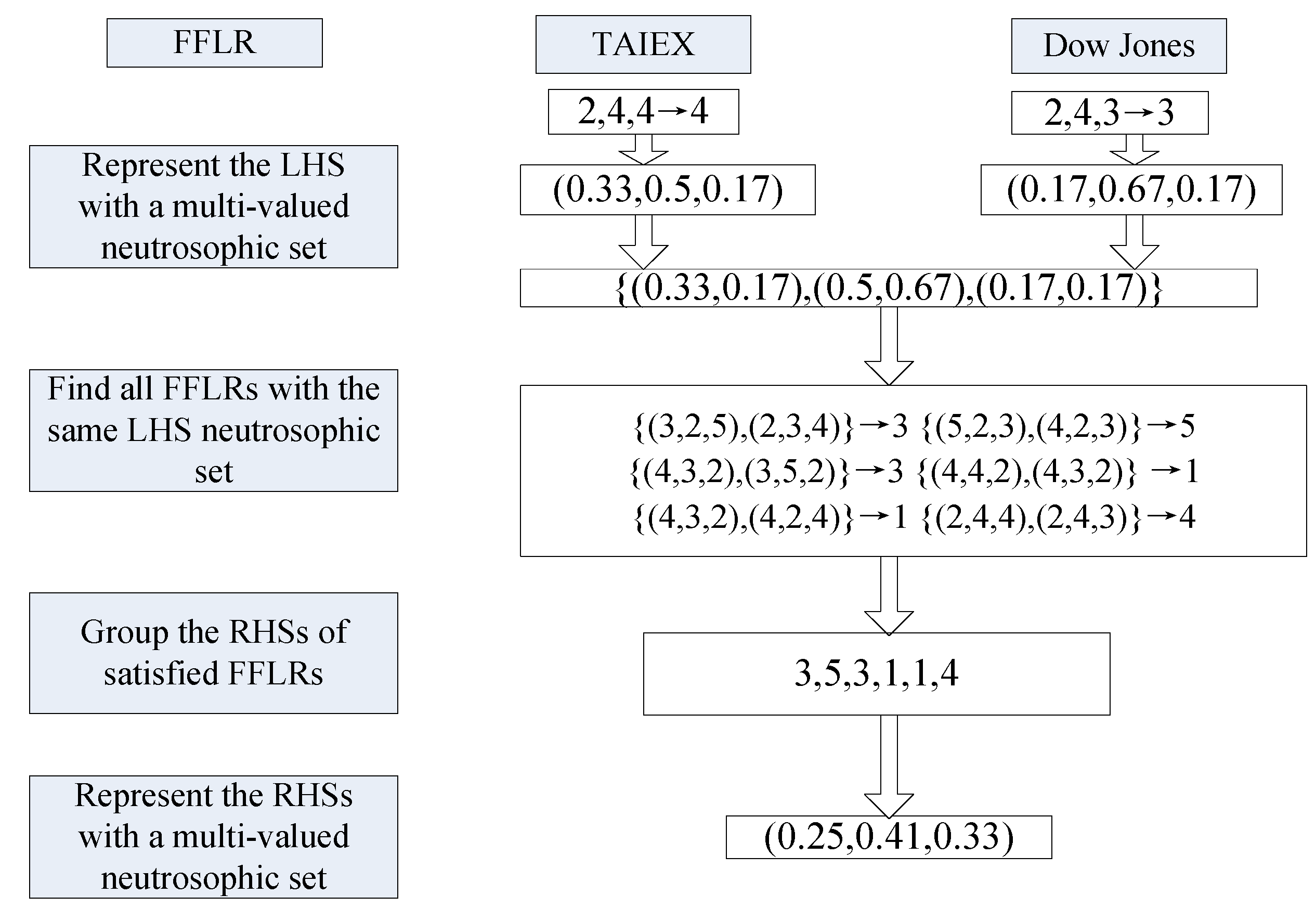
Figure 3.
Forecasting results from 1 November 2004 to 30 December 2004.
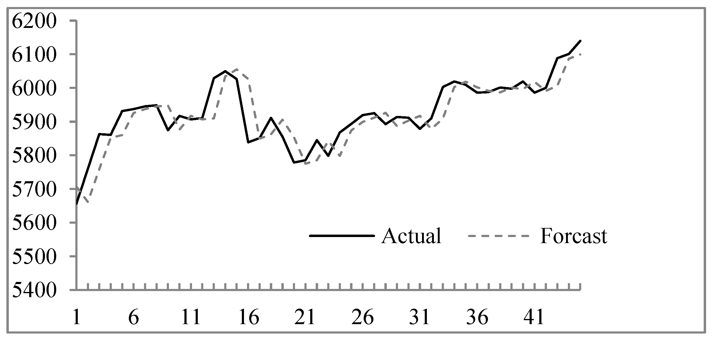
Figure 4.
The stock market fluctuation for TAIEX test dataset (1998–2006).
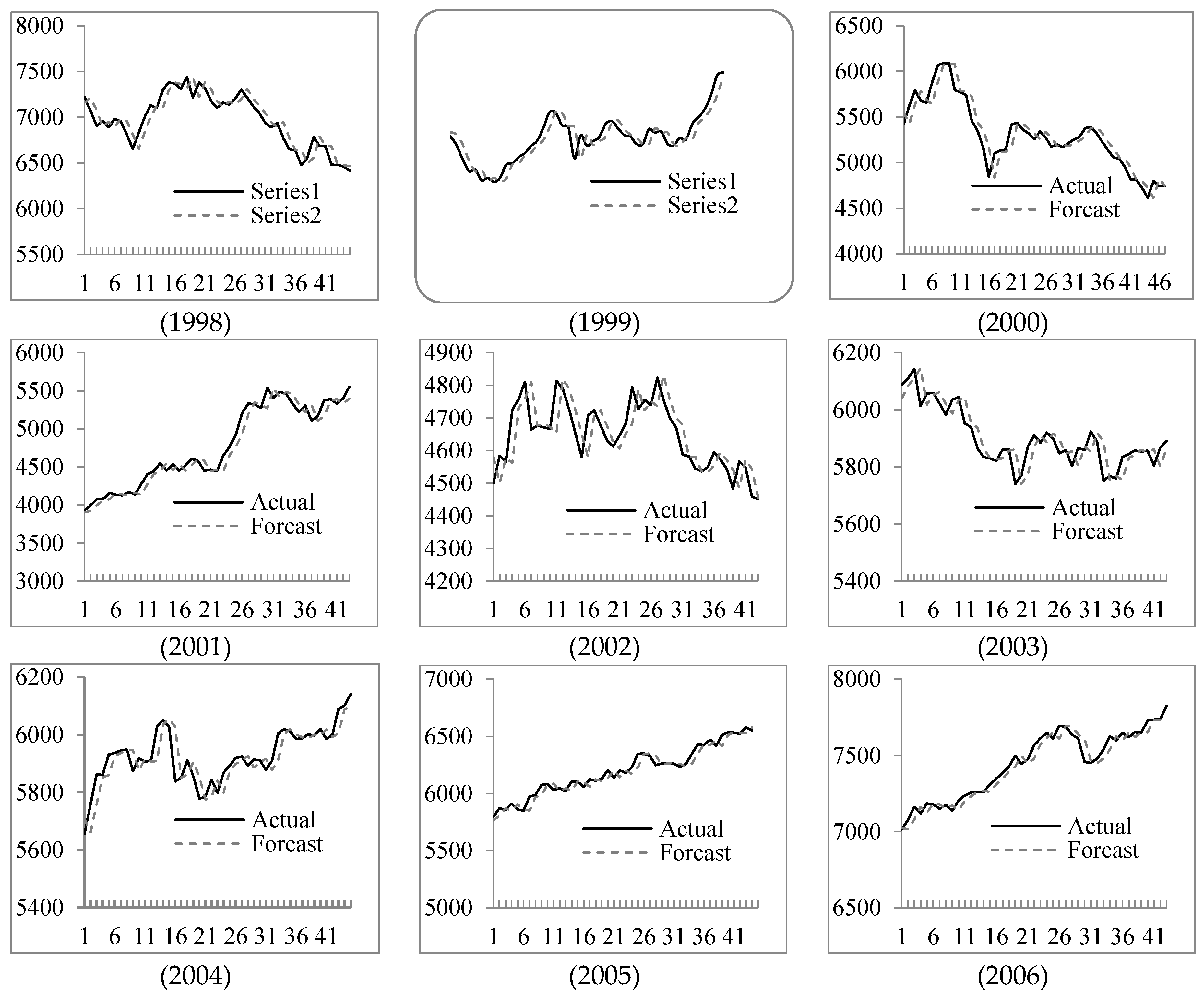
Table 1.
Forecasting results from 1 November 2004 to 30 December 2004.
| Date (YYYY/MM/DD) | Actual | Forecast | (Forecast − Actual)2 | Date (YYYY/MM/DD) | Actual | Forecast | (Forecast − Actual)2 |
|---|---|---|---|---|---|---|---|
| 2004/11/1 | 5656.17 | 5708.72 | 2761.50 | 2004/12/2 | 5867.95 | 5798.62 | 4806.65 |
| 2004/11/2 | 5759.61 | 5678.51 | 6576.48 | 2004/12/3 | 5893.27 | 5867.95 | 641.10 |
| 2004/11/3 | 5862.85 | 5781.95 | 9575.93 | 2004/12/6 | 5919.17 | 5926.79 | 58.01 |
| 2004/11/4 | 5860.73 | 5862.85 | 10,658.50 | 2004/12/7 | 5925.28 | 5908.00 | 298.68 |
| 2004/11/5 | 5931.31 | 5860.73 | 4981.54 | 2004/12/8 | 5892.51 | 5925.28 | 1073.87 |
| 2004/11/8 | 5937.46 | 5908.97 | 811.94 | 2004/12/9 | 5913.97 | 5896.98 | 288.70 |
| 2004/11/9 | 5945.2 | 5959.80 | 213.29 | 2004/12/10 | 5911.63 | 5880.45 | 971.99 |
| 2004/11/10 | 5948.49 | 5945.20 | 10.82 | 2004/12/13 | 5878.89 | 5933.97 | 3034.30 |
| 2004/11/11 | 5874.52 | 5970.83 | 0.25 | 2004/12/14 | 5909.65 | 5901.23 | 70.82 |
| 2004/11/12 | 5917.16 | 5874.52 | 1818.17 | 2004/12/15 | 6002.58 | 5931.99 | 4982.31 |
| 2004/11/15 | 5906.69 | 5917.16 | 109.62 | 2004/12/16 | 6019.23 | 6024.92 | 32.43 |
| 2004/11/16 | 5910.85 | 5906.69 | 17.31 | 2004/12/17 | 6009.32 | 6019.23 | 98.21 |
| 2004/11/17 | 6028.68 | 5902.36 | 15,956.97 | 2004/12/20 | 5985.94 | 5998.15 | 149.03 |
| 2004/11/18 | 6049.49 | 6062.20 | 161.46 | 2004/12/21 | 5987.85 | 6008.28 | 417.57 |
| 2004/11/19 | 6026.55 | 6083.01 | 3187.36 | 2004/12/22 | 6001.52 | 6010.19 | 13.49 |
| 2004/11/22 | 5838.42 | 6004.21 | 27,484.83 | 2004/12/23 | 5997.67 | 6023.86 | 686.15 |
| 2004/11/23 | 5851.1 | 5844.01 | 50.32 | 2004/12/24 | 6019.42 | 6020.01 | 0.35 |
| 2004/11/24 | 5911.31 | 5856.69 | 2983.77 | 2004/12/27 | 5985.94 | 6019.42 | 1120.91 |
| 2004/11/25 | 5855.24 | 5888.97 | 1137.41 | 2004/12/28 | 6000.57 | 6008.28 | 59.51 |
| 2004/11/26 | 5778.65 | 5846.75 | 4637.49 | 2004/12/29 | 6088.49 | 6022.91 | 4300.15 |
| 2004/11/29 | 5785.26. | 5771.05 | 201.84 | 2004/12/30 | 6100.86 | 6080.00 | 435.18 |
| 2004/11/30 | 5844.76 | 5776.88 | 4607.58 | 2004/12/31 | 6139.69 | 6092.37 | 2239.27 |
| 2004/12/1 | 5798.62 | 5850.35 | 2675.59 | RMSE | 53.01 | ||
RMSE: root of the mean squared error.
Table 2.
Comparison of forecasting errors for different nth-orders.
| n | 1 | 3 | 5 | 7 | 9 |
|---|---|---|---|---|---|
| RMSE | 54.65 | 53.01 | 55.60 | 55.06 | 54.43 |
Table 3.
RMSEs of forecast errors for TAIEX 1998 to 2006.
| Year | 1998 | 1999 | 2000 | 2001 | 2002 | 2003 | 2004 | 2005 | 2006 |
|---|---|---|---|---|---|---|---|---|---|
| RMSE | 115.45 | 105.49 | 129.11 | 113.69 | 67.12 | 53.6 | 53.01 | 53.49 | 51.90 |
Table 4.
A comparison of RMSEs for different methods for forecasting the TAIEX2004.
| Methods | RMSE |
|---|---|
| Huarng et al.’s method [41] | 73.57 |
| Chen and Kao’s method [42] | 58.17 |
| Cheng et al.’s method [43] | 54.24 |
| Chen et al.’s method [44] | 56.16 |
| Chen and Chang’s method [45] | 60.48 |
| Chen and Chen’s method [46] | 61.94 |
| Yu and Huarng’s method [47] | 55.91 |
| The proposed method | 53.01 |
Table 5.
RMSEs of forecast errors for the Shanghai Stock Exchange Composite Index (SHSECI) from 2004 to 2015.
Table 5.
RMSEs of forecast errors for the Shanghai Stock Exchange Composite Index (SHSECI) from 2004 to 2015.
| Year | 2004 | 2005 | 2006 | 2007 | 2008 | 2009 | 2010 | 2011 | 2012 | 2013 | 2014 | 2015 |
|---|---|---|---|---|---|---|---|---|---|---|---|---|
| RMSE | 13.54 | 9.03 | 37.68 | 108.17 | 50.88 | 50.22 | 46.08 | 28.1 | 25.36 | 20.19 | 52.79 | 55.80 |
© 2018 by the authors. Licensee MDPI, Basel, Switzerland. This article is an open access article distributed under the terms and conditions of the Creative Commons Attribution (CC BY) license (http://creativecommons.org/licenses/by/4.0/).
Share and Cite
MDPI and ACS Style
Guan, H.; He, J.; Zhao, A.; Dai, Z.; Guan, S. A Forecasting Model Based on Multi-Valued Neutrosophic Sets and Two-Factor, Third-Order Fuzzy Fluctuation Logical Relationships. Symmetry 2018, 10, 245. https://doi.org/10.3390/sym10070245
AMA Style
Guan H, He J, Zhao A, Dai Z, Guan S. A Forecasting Model Based on Multi-Valued Neutrosophic Sets and Two-Factor, Third-Order Fuzzy Fluctuation Logical Relationships. Symmetry. 2018; 10(7):245. https://doi.org/10.3390/sym10070245
Chicago/Turabian StyleGuan, Hongjun, Jie He, Aiwu Zhao, Zongli Dai, and Shuang Guan. 2018. "A Forecasting Model Based on Multi-Valued Neutrosophic Sets and Two-Factor, Third-Order Fuzzy Fluctuation Logical Relationships" Symmetry 10, no. 7: 245. https://doi.org/10.3390/sym10070245
Note that from the first issue of 2016, this journal uses article numbers instead of page numbers. See further details here.