Sampling Based Histogram PCA and Its Mapreduce Parallel Implementation on Multicore

Abstract

In existing principle component analysis (PCA) methods for histogram-valued symbolic data, projection results are approximated based on Moore’s algebra and fail to reflect the data’s true structure, mainly because there is no precise, unified calculation method for the linear combination of histogram data. In this paper, we propose a new PCA method for histogram data that distinguishes itself from various well-established methods in that it can project observations onto the space spanned by principal components more accurately and rapidly by sampling through a MapReduce framework. The new histogram PCA method is implemented under the same assumption of “orthogonal dimensions for every observation” with the existing literatures. To project observations, the method first samples from the original histogram variables to acquire single-valued data, on which linear combination operations can be performed. Then, the projection of observations can be given by linear combination of loading vectors and single-valued samples, which is close to accurate projection results. Finally, the projection is summarized to histogram data. These procedures involve complex algorithms and large-scale data, which makes the new method time-consuming. To speed it up, we undertake a parallel implementation of the new method in a multicore MapReduce framework. A simulation study and an empirical study confirm that the new method is effective and time-saving.

1. Introduction

Generalized Principal Component Analysis (PCA) is an important research tool in the Symbolic Data Analysis (SDA) [1]. PCA is a statistical procedure that uses orthogonal transformation to convert a set of observations of possibly correlated variables into a set of values of linearly uncorrelated variables called principal components (PCs) [2,3,4]. PCA is commonly used for dimension reduction [5,6] by specifying a few PCs that account for as much of the variability in the original dataset as possible. It is well known that PCA has been primarily developed for single-valued variables. However, the explosion of big data from a wide range of application domains presents new challenges for traditional PCA, as it is difficult to gain insight from mass observation even in a low-dimensional space. Symbolic data analysis [7,8,9,10] has developed a new path for solving this problem.

Symbolic data was first introduced by [7] and aims to summarize large-scale data with conceptual observations described by symbolic descriptors, such as interval data, histogram, and continuous distribution data. Application fields of symbolic data include economic management, finance, and sociodemographic surveys. Thus, some researchers devoted themselves to studying new PCA methods for symbolic data. Here, we are interested in PCA for histogram data, where each variable value for each unit is a set of weights associated with the bins of variable values. The weights can be considered to be the frequency or probability of their associated bin for the corresponding unit. The sum of the weights is equal to 1.

Several studies contribute to the extension of PCA to histogram data. Reference [11] attempted to analyze a symbolic dataset for dimensionality reduction when the features are of histogram type. This approach assumes that the modal variables have the same number of ordered bins and uses the PCA of tables associated with each bin. References [12,13] assumed that the same number of bins was ordered for each variable. References [1,14] proposed approaches based on distributions of histogram transformation, which is not possible in the case of nonordinal bins. Nevertheless, the Ichino method solves this case by ranking bins by their frequency among the whole population of individuals. Reference [15] presented a strategy for extending standard PCA to histogram data. This method uses metabins that mix bins from different bar charts and enhance interpretability. Then it proposes Copular PCA to handle the probabilities and underlying dependencies. The method presented by [1] builds metabins and metabin trajectories for each individual from the nominal histogram variables. Reference [15] also proved that the method proposed by [1] is an alternate solution to Copular PCA. Reference [16] expressed an accurate distribution of linear combination of quantitative symbolic variables by convolutions of their probability distribution functions. Reference [17] use Multiple Factor Analysis (MFA) approach for the analysis of data described by distributional variables. Each distributional variable induces a set new numeric variable related to the quantiles of each distribution. Reference [18] deals with the current situation of histogram use through histogram PCA.

Despite the number of experts who study PCA for histogram data, there are still many challenging issues that have not been fully addressed in previous publications. In PCA methods for histogram data, projection results are approximated based on Moore’s algebra [19] and fail to reflect the data’s true structure, mainly because methods of linear combinations of histogram data are imprecise and not unified. The PSPCA method proposed by [16] can obtain precise projections, but the process of calculating convolutions is very complicated and time consuming, requiring a more efficient method of PCA for histogram data.

In this paper, we investigate a sampling-based PCA method for histogram data to solve the dimension reduction problem of histogram data. This method can project observations onto the space spanned by PCs more accurately and rapidly using a MapReduce framework. Assuming orthogonal dimensions for every observation [20], as in existing literature, to project observations onto the space spanned by PCs, we first sample from the original histogram variables to acquire single-valued data on which linear combination operations can be performed. Then, the projection of observations can be described by a linear combination of loading vectors and single-valued samples. Lastly, the projection is summarized to histogram data. As random sampling is used in this process, the projection results of different samplings may be different, resulting in the projection results of the proposed method being only close to accurate projections. However, we have proved that for a sufficiently large sample size, the projection results tend towards stability and are close to the accurate projections.

Because this method uses complex algorithms and large-scale data, it is quite time consuming. To speed up the method, we undertake a parallel implementation of the new method through a multicore MapReduce framework. MapReduce is a popular parallel programming model for cloud computing platforms and has been effective in processing large datasets using multicore or multiprocessor systems [21,22,23,24,25]. We conducted a simulation experiment to confirm that the new method is effective and can be substantially accelerated.

It should be emphasized that we only propose the MapReduce framework for sampling-based histogram PCA for big data. When there is sufficient data, we can use a big data platform like Hadoop and adopt parallel computing methods, such as GPU computing and MPI (Message Passing Interface). In this paper, we simply consider a multicore MapReduce parallel implementation.

The remainder of this paper is organized as follows. In Section 2, we propose a sampling-based Histogram PCA method. Section 3 describes the implementation of the new method in a multicore MapReduce framework. Next, in Section 4, a simulation study of the new method and its parallel implementation are presented. We also compare the execution times of serial and parallel processing. In Section 5, we report the results of our empirical study. Finally, Section 6 outlines our conclusions.

2. Sampling-Based Histogram PCA

In this section, we first define the inner product operator for histogram-valued data, then derive histogram PCA, and finally project the observations onto the space spanned by principal components using sampling.

2.1. Basic Operators

Let $\mathbf{X}$ be a data matrix that can be expressed as a vector of observations or of variables.

$$\mathbf{X}={[{\mathbf{e}}_1^T\dots {\mathbf{e}}_n^T]}^T=[{\mathbf{X}}_1\dots {\mathbf{X}}_p],$$

(1)

where ${\mathbf{e}}_i=(x_{i1},\dots ,x_{ip}),i=1,\dots ,n$ denotes the ith observation and ${\mathbf{X}}_j=(x_{1j},\dots$, $x_{nj}{)}^T,j=1,\dots ,p$ denotes the jth variable. Additionally, the random variable $x_{ij}$ represents the jth variable of the ith observation, with realization $x_{ij}$ in the classical case and ${\xi }_{ij}$ in the symbolic case.

Next, we give the empirical distribution functions and descriptive statistics for histogram data. For further detail, refer to [9,26].

Let ${\mathbf{e}}_i$, i = 1, …, n, be a random sample. Let the jth variable have a histogram-valued realization ${\xi }_{ij}$,

$${\xi }_{ij}=\{[a_{ij}^1,b_{ij}^1),p_{ij}^1;[a_{ij}^2,b_{ij}^2),p_{ij}^2;\dots ;[a_{ij}^{s_{ij}},b_{ij}^{s_{ij}}],p_{ij}^{s_{ij}}\}$$

(2)

where $[a_{ij}^l,b_{ij}^l)$ is the lth subinterval of ${\xi }_{ij}$ and $p_{ij}^l$ is its associated relative frequency. Let $s_{ij}$ denote the number of subintervals in ${\xi }_{ij}$. Then, $a_{ij}^l\le b_{ij}^l$ for all l = 1, …,$s_{ij}$, and ${\sum }_{l=1}^{s_{ij}}{p}_{ij}^l=1$.

Reference [27] extended the empirical distribution function derived by [26] for interval data to histogram data. Based on the assumption that all values within each subinterval $[a_{ij}^1,b_{ij}^1)$ are uniformly distributed, they defined the empirical distribution of a point $W_s$ within subinterval $[a_{ij}^1,b_{ij}^1)$ as

$$P(W_s\le w)=\left\{\begin{array}{cc}0,\hfill & w<a_{ij}^l,\hfill \\ (w-a_{ij}^l)/(b_{ij}^l-a_{ij}^l),\hfill & a_{ij}^l\le w<b_{ij}^l,\hfill \\ 1,\hfill & b_{ij}^l\le w.\hfill \end{array}\right.$$

(3)

Furthermore, assume that each object is equally likely to be observed with probability $1/n$; then, the empirical distribution function of W is

$$F_W(w)=\frac{1}{n}{\displaystyle \sum _{i=1}^n}[\sum _{l:w\in {\xi }_{ij}^l}{p}_{ij}^l(w-a_{ij}^l)/(b_{ij}^l-a_{ij}^l)+\sum _{l:w\ge b_{ij}^l}{p}_{ij}^l],$$

(4)

where ${\xi }_{ij}^l=[a_{ij}^1,b_{ij}^1)$. The empirical density function of W is defined as

$$f_W(w)=\frac{1}{n}{\displaystyle \sum _{i=1}^n}\sum _{l:w\in {\xi }_{ij}^l}{p}_{ij}^l/(b_{ij}^l-a_{ij}^l).$$

(5)

The symbolic sample mean derived from the density function shown in Equation (5) is

$$\overline{W}=\frac{1}{2n}{\displaystyle \sum _{i=1}^n}{\displaystyle \sum _{l=1}^{s_{ij}}}{p}_{ij}^l(a_{ij}^l+b_{ij}^l).$$

(6)

Accordingly, the centralization of $x_{ij}$ is given by

$$\widetilde{x_{ij}}=x_{ij}-\overline{W}.$$

(7)

After centralization, the symbolic sample variance and covariance are, respectively,

$$S^2=\frac{1}{3n}{\displaystyle \sum _{i=1}^n}{\displaystyle \sum _{l=1}^{s_{ij}}}{p}_{ij}^l[{(a_{ij}^l)}^2+a_{ij}^l{b}_{ij}^l+{(b_{ij}^l)}^2],$$

(8)

and

$$S_{ij}=\frac{1}{4n}{\displaystyle \sum _{i=1}^n}[{\displaystyle \sum _{l=1}^{s_{ik}}}{p}_{ik}^l(a_{ik}^l+b_{ik}^l)][{\displaystyle \sum _{l=1}^{s_{jk}}}{p}_{jk}^l(a_{jk}^l+b_{jk}^l)],i\ne j.$$

(9)

2.2. The PCA Algorithm of Histogram Data

Based on the operators above, we begin to derive histogram-valued PCs. For simplicity of notation, we assume that all histogram-valued data units have been centralized.

The kth histogram-valued PC ${\mathbf{Y}}_k(k=1\dots p)$ is a linear combination of ${\mathbf{X}}_1,{\mathbf{X}}_2,\dots ,{\mathbf{X}}_p$,

$${\mathbf{Y}}_k={\mathbf{Xu}}_k={\displaystyle \sum _{j=1}^p}{u}_{jk}{\mathbf{X}}_j,$$

(10)

where ${\mathbf{u}}_k={(u_{1k}\dots u_{pk})}^T\in {\mathbb{R}}^p$ is subject to ${\mathbf{u}}_k^T{\mathbf{u}}_k=1$ and ${\mathbf{u}}_k^T{\mathbf{u}}_l=0,\forall l\ne k$. Then, the symbolic sample variance of ${\mathbf{Y}}_k(k=1\dots p)$ can be derived from

$$S_{{\mathbf{Y}}_k}^2=(u_{1k},u_{2k},\dots ,u_{pk})\left(\begin{array}{cccc}{S}_1^2& S_{12}& \cdots & S_{1p}\\ S_{21}& S_2^2& \cdots & S_{2p}\\ ⋮& ⋮& \ddots & ⋮\\ S_{p1}& S_{p2}& \cdots & S_p^2\end{array}\right)\left(\begin{array}{c}{u}_{1k}\\ u_{2k}\\ ⋮\\ u_{pk}\end{array}\right)={\mathbf{u}}_k^T\mathbf{\Sigma }{\mathbf{u}}_k,$$

(11)

where $\mathbf{\Sigma }$ represents the sample covariance matrix as ${\mathbf{X}}_1,{\mathbf{X}}_2,\dots ,{\mathbf{X}}_p$, in which $S_i^2$ and $S_{ij}(i,j=1\dots p)$ are present in Equations (8) and (9).

The following process is the same as that for classical PCA. (for details, see the original sources).

Set ${\mathbf{u}}_1,{\mathbf{u}}_2,\dots ,{\mathbf{u}}_m$ as the eigenvectors of $\mathbf{\Sigma }$, corresponding to the eigenvalues ${\lambda }_1⩾{\lambda }_2⩾\dots ⩾{\lambda }_m$. The derivation of PC coefficients is transformed into the eigendecomposition of the covariance matrix. The contribution rate($CR$) of the mth PC to the total variance can be measured by

$$C{R}_m=\frac{S_{{\mathbf{Y}}_m}^2}{{\displaystyle \sum _{j=1}^p}{S}_{{\mathbf{Y}}_j}^2}=\frac{{\lambda }_m}{{\displaystyle \sum _{j=1}^p}{\lambda }_j}.$$

(12)

2.3. The Projection Process

In existing PCA methods for histogram data, the projection results are approximated based on Moore’s algebra [19] and fail to reflect true data structures, mainly because there are no precise, unified methods for linearly combining histogram data.

In this paper, we project observations onto the space spanned by PCs with a sampling method. Using the concept of symbolic data, histogram-valued data can be generated from a mass of numerical data. Retroactively, we can also sample from histogram-valued data to obtain numerical data on which linear combination operations can be performed. As PC coefficients and numerical variables corresponding to the original histogram-valued variables are obtained, we can calculate the numerical projections by linearly combining them. Then, histogram-valued projections of the original observations can be summarized from numerical projections.

Let $x_{ij}$ represent the ith observation unit of the jth variable ${\mathbf{X}}_j$ in histogram-valued matrix $\mathbf{X}$. ${\xi }_{ij}$ in Equation (2) is a realization of $x_{ij}$. Based on the assumption that all values within each subinterval $[a_{ij}^1,b_{ij}^1)$ are uniformly distributed, to obtain numerical data corresponding to ${\xi }_{ij}$, we select $m_i$ samples from those subintervals of ${\xi }_{ij}$ through random sampling. To maintain the coherence of the numerical sample matrix, the sample sizes of different variables from the same observation are assumed to be equal. After the random sampling process, the numerical sample matrix corresponding to the original histogram-valued matrix, which we call matrix $\mathbf{P}$, can be obtained. As the dimension of $\mathbf{X}$ is $n\times p$, the dimension of $\mathbf{P}$ is ${\displaystyle \sum _{i=1}^n}{m}_i\times p$.

According to Equation (10), the kth numerical PC ${\mathbf{NY}}_k(k=1\dots p)$ is a linear combination of ${\mathbf{P}}_1,{\mathbf{P}}_2,\dots ,{\mathbf{P}}_p$,

$${\mathbf{NY}}_k=\mathbf{P}{\mathbf{u}}_k={\displaystyle \sum _{j=1}^p}{u}_{jk}{\mathbf{P}}_j.$$

(13)

The calculation in Equation (13) can be performed because ${\mathbf{P}}_1,{\mathbf{P}}_2,\dots ,{\mathbf{P}}_p$ are numerical variables. The projection approach in Equation (13) is similar to the classic PCA approach. Finally, we obtain histogram-valued PCs through generating numerical PCs. In this way, histogram-valued observations are successfully projected onto the space spanned by PCs.

The above analysis can be summarized by the following algorithm:

• Step 1: Centralize the histogram-valued matrix $\mathbf{X}$ in Equation (1) and keep the notations consistent for simplicity.
• Step 2: Calculate the covariance matrix $\mathbf{\Sigma }$ of $\mathbf{X}$ using Equations (8) and (9).
• Step 3: Eigendecompose $\mathbf{\Sigma }$ for orthonormalized eigenvectors ${\mathbf{u}}_1,{\mathbf{u}}_2,\dots ,{\mathbf{u}}_m(m\le p)$ in accordance with the eigenvalues ${\lambda }_1⩾{\lambda }_2⩾\dots ⩾{\lambda }_m$, which are PC coefficients and PC variances, respectively.
• Step 4: Obtain numerical matrix $\mathbf{P}$ through random sampling from $\mathbf{X}$.
• Step 5: Compute the numerical PCs ${\mathbf{NY}}_1,{\mathbf{NY}}_2,\dots ,{\mathbf{NY}}_m$ using Equation (13).
• Step 6: Generate histogram-valued PCs ${\mathbf{Y}}_1,{\mathbf{Y}}_2,\dots ,{\mathbf{Y}}_m$ by summarizing numerical PCs ${\mathbf{NY}}_1,{\mathbf{NY}}_2$, $\dots ,{\mathbf{NY}}_m$.

During this procedure, it is crucial to guarantee that any column of the matrix $\mathbf{P}$ obtained by sampling has the same distribution as the corresponding column in $\mathbf{X}$, or that the distance between these two distributions is small enough to be negligible. Considering the empirical cumulative distribution approximates the true cumulative distribution favorably, we can determine that the difference between these two distributions converges as the sample size goes to infinity. Here, we give some key conclusions from the perspective of asymptotic theory.

Kolmogorov-Smirnov distance is a useful measure of global closeness between distributions $F_m(x)$ and $F(x)$

$$D_m=\underset{-\infty <x<\infty }{sup}|F_m(x)-F(x)|.$$

(14)

The asymptotic properties of Kolmogorov-Smirnov distance $D_m$ have been studied and many related conclusions have been built. Extreme fluctuations in the convergence of $D_m$ to 0 can be characterized by [28]

$${\overline{lim}}_{m\to \infty }\frac{m^{1/2}{D}_m}{{(2loglogm)}^{1/2}}=\underset{x}{sup}\sqrt{F(x)(1-F(x))}.$$

(15)

Here, we deal with histogram data, in which case $F(x)$ is not continuous; thus, we cannot give ${sup}_x\sqrt{F(x)(1-F(x))}$. According to Equation (15), $D_m$ converges with a rate slower than $m^{-1/2}$ by a factor ${(loglogm)}^{1/2}.$

From the pointwise closeness of $F_m(x)$ to $F(x),$ we can easily observe that

$$F_m(x)isAN\left(F(x),\frac{F(x)[1-F(x)]}{n}\right),forfixedx,$$

(16)

where $AN$ is asymptotic normality.

Therefore, global and local differences between the histogram obtained from sampling data and the original can be controlled when the sample size is large, illustrating the feasibility of the proposed sampling method. It should be noted that the original histogram data, which is not continuous, is treated as the true distribution, but the conclusions above can cover discontinuous cases, although the formula expression may be complex. Related theoretical issues will be considered in the future.

3. MapReduce for Multicore, Sampling-Based Histogram PCA

The sampling-based histogram PCA approach presented in Section 2 involves complex algorithms and large-scale data, which makes the method time-consuming and degrades its computation efficiency. To speed up the method, we undertake its parallel implementation using a multicore MapReduce framework in this section.

MapReduce is a programming model for processing large datasets with a parallel, distributed algorithm on a cluster. A MapReduce program is composed of a map procedure that filters and sorts data and a reduce procedure that performs a summary operation [21]. Reference [22] show that algorithms that can be written in a “summation form” can be easily parallelized on multicore computers. Coincidentally, Equations (8), (9) and (13) are written in this form. In addition, the random sampling procedure can also be parallelized. Consequently, we adapt the MapReduce paradigm to implement our histogram PCA algorithm.

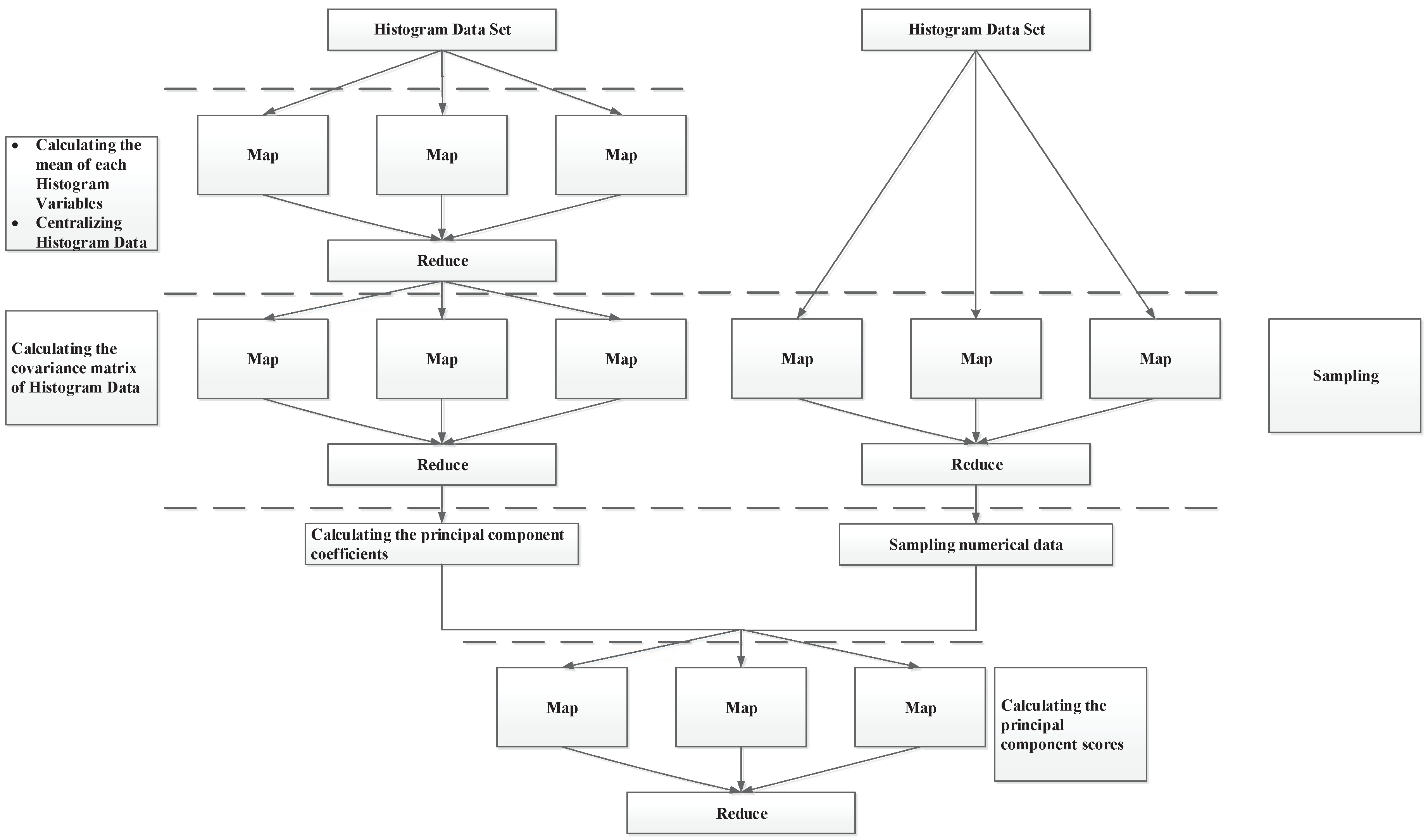
The multicore MapReduce frame for histogram PCA is presented in Figure 1, which shows a high- level view of our architecture and how it processes the data. In Step 1, the MapReduce engine calculates the mean of each histogram variable using Equation (6) using pseudocode shown in Algorithm 1.

Algorithm 1 MapReduce for calculating the mean of each histogram variable
1:	function map1 ($key,value$)
2:
3:	$//$$key$: row ID of the observation in $\mathbf{X}$
4:
5:	$//$$value$: observations in $\mathbf{X}$
6:
7:	for each element ${\xi }_{ij}$ in $value$ do
8:
9:	$su{m}_{ij}=\frac{1}{2}{\displaystyle \sum _{l=1}^{s_{ij}}}{p}_{ij}^l(a_{ij}^l+b_{ij}^l)$
10:
11:	end for
12:
13:	return ($coordinate,su{m}_{ij}$)$//$ $coordinate$: coordinates of elements in $\mathbf{X}$
14:
15:	end function
16:
17:	function reduce1 ($coordinate,su{m}_{ij}$)
18:
19:	for $j=1\to p$ do
20:
21:	${\overline{W}}_j=\frac{1}{n}{\displaystyle \sum _{i=1}^n}su{m}_{ij}$ $//$ Calculating the mean of each histogram variable
22:
23:	end for
24:
25:	return ($column$_$id,{\overline{W}}_j$)
26:
27:	end function

Then, the variables are centralized using Equation (7). Every variable has its own engine instance, and every MapReduce task is delegated to its engine. Similarly, calculating the covariance matrix of histogram data using Equations (8) and (9) in Step 2, random sampling from $\mathbf{X}$ in Step 4, and computing the numerical principal components ${\mathbf{NY}}_1,{\mathbf{NY}}_2,\dots ,{\mathbf{NY}}_m$ using Equation (13) in Step 5 can also be delegated to MapReduce engines. The map and reduce functions are presented in Algorithms 2 and 3.

Algorithm 2 MapReduce for centralizing histogram data and calculating the covariance matrix of histogram data
1:	function map2 ($key,value$)
2:
3:	$//$ $key$: row ID of the observation in $\mathbf{X}$
4:
5:	$//$ $value$: observations in $\mathbf{X}$
6:
7:	for each element ${\xi }_{ij}$ in $value$ do
8:
9:	${\xi }_{ij}={\xi }_{ij}-{\overline{W}}_j$ $//$Centralizing histogram data
10:
11:	$su{m}_{ij}=\frac{1}{2}{\displaystyle \sum _{l=1}^{s_{ij}}}{p}_{ij}^l(a_{ij}^l+b_{ij}^l)$
12:
13:	end for
14:
15:	return ($coordinate,su{m}_{ij}$)$//$ $coordinate$: coordinates of elements in $\mathbf{X}$
16:
17:	end function
18:
19:	function reduce2 ($coordinate,su{m}_{ij}$)
20:
21:	for $i=1\to p$ do
22:
23:	for $j=1\to p$ do
24:
25:	if $i==j$ then
26:
27:	$S_{ij}=\frac{1}{3n}{\displaystyle \sum _{i=1}^n\sum _{l=1}^{s_{ij}}}{p}_{ij}^l[{(a_{ij}^l)}^2+a_{ij}^l{b}_{ij}^l+{(b_{ij}^l)}^2]$
28:
29:	else
30:
31:	$S_{ij}=\frac{1}{4n}{\displaystyle \sum _{i=1}^n}[{\displaystyle \sum _{l=1}^{s_{ik}}}{p}_{ik}^l(a_{ik}^l+b_{ik}^l)][{\displaystyle \sum _{l=1}^{s_{jk}}}{p}_{jk}^l(a_{jk}^l+b_{jk}^l)]$
32:
33:	$//$ Calculating the covariance matrix of histogram data
34:
35:	end if
36:
37:	end for
38:
39:	end for
40:
41:	return ($cov$_$id,S_{ij}$)$//$ $cov$_$id$: coordinates of elements in $\mathbf{S}$
42:
43:	end function

Algorithm 3 MapReduce for sampling-based histogram PCA
1:	function map3 ($key,value$)
2:
3:	$//$ $key$: row ID of the observation in $\mathbf{X}$
4:
5:	$//$ $value$: observations in $\mathbf{X}$
6:
7:	for each element ${\xi }_{ij}$ in $value$ do
8:
9:	${\mathbf{P}}_{ij}\leftarrow$Randomly sampling numerical data from ${\xi }_{ij}$, the sample size is K.
10:
11:	end for
12:
13:	return ($coordinate,{\mathbf{P}}_{ij}$)
14:
15:	end function
16:
17:	function reduce3 ($coordinate,{\mathbf{P}}_{ij}$)
18:
19:	for each element ${\mathbf{P}}_{ij}$ in $\mathbf{P}$ do
20:
21:	${\mathbf{NY}}_{ik}={\displaystyle \sum _{j=1}^p}{u}_{jk}{\mathbf{P}}_{ij}$
22:
23:	$//$Calculating the ith observation of the kth numerical PC
24:
25:	${\mathbf{Y}}_{ik}\leftarrow$ Summarizing numerical PCs to obtain histogram PCs
26:
27:	end for
28:
29:	return ($pc$_$id,{\mathbf{Y}}_k$)$//$ ${\mathbf{Y}}_k$: the kth histogram PC
30:
31:	end function
32:

4. Simulation Study

To analyze the performance of the new histogram PCA method and demonstrate whether MapReduce parallelization can speed it up, we carried out a simulation study involving three examples.

$$\{U(1,3),N(1,1),{\chi }^2(1),lnN(0,0.5),-lnN(0,0.5)\}.$$

Of the examples, Example 1 investigates the histogram PCA accuracy in Section 2.2, Example 2 evaluates the precision of the sampling-based projection process of histogram PCA in Section 2.3, and Example 3 compares the method’s execution time in parallel and serial systems.

The environment in which we conducted experiments is a PC with 8 Core Intel i7-6700K 4.00 GHz CPU and 8 GB RAM running Windows 7.

4.1. Example 1

With Example 1, we aim to investigate the accuracy of the histogram PCA algorithm. The simulated symbolic data tables are built as in [29]. Based on the concept of symbolic variables, to obtain n observations associated with a histogram-valued variable ${\mathbf{X}}_k$, we simulate K real values $x_{ik}^{NUM}$ corresponding to each unit. These values are then organized in histograms that represent the empirical distribution for each unit. The distribution of the microdata that allow histogram generation, corresponding to each observation of the variables ${\mathbf{X}}_k(k=1\dots p)$, is randomly selected from a mixture of distributions. Without loss of generality, in all observations, the widths of the subintervals in each histogram are the same.

Thus, we generate n histogram observations and the corresponding $n\times K$ single-value data points. The single-value data points can be viewed as the original data, which we aim to approximate using histogram-valued data. Consequently, experimental PCA results obtained from single-value data can work as an evaluation benchmark for the histogram PCA algorithm.

The detailed process of Example 1 is as follows:

(1) Generate a synthetic histogram dataset $\mathbf{X}$ with p variables and n observations and the corresponding single-value dataset, denoted as ${\mathbf{X}}^{NUM}$.

(2) Adopt the new histogram PCA method on $\mathbf{X}$ and perform classical PCA on ${\mathbf{X}}^{NUM}$. The obtained PC coefficients are denoted as ${\mathbf{u}}_j$ and ${\mathbf{u}}_j^{NUM}$, and the corresponding PC variances are represented by ${\lambda }_j$ and ${\lambda }_j^{NUM}$, $j=1,2,\dots ,p$.

(3) Compute the following two indicators [30]:

(a) Absolute cosine value ($ACV$) of PC coefficients:

$$ACV({\mathbf{u}}_j)=|\frac{{({\mathbf{u}}_j)}^T{\mathbf{u}}_j^{NUM}}{\parallel {\mathbf{u}}_j\parallel \parallel {\mathbf{u}}_j^{NUM}\parallel }|.$$

(17)

Since cosine measures the angle between two vectors, $ACV$ describes the similarity between PC coefficients ${\mathbf{u}}_j$ and the benchmark ${\mathbf{u}}_j^{NUM}$. A higher $ACV$ indicates a better performance of the new histogram PCA method. (b) Relative error ($RE$) of PC variances:

$$RE({\lambda }_j)=|\frac{{\lambda }_j-{\lambda }_j^{NUM}}{{\lambda }_j^{NUM}}|.$$

(18)

Taking PC variances obtained from ${\mathbf{X}}^{NUM}$ as a benchmark, the lower the $RE$ is, the better the new histogram PCA method has performed.

The parameters for the experiments are set as follows: $n=30,p=3,K=50,100,500$, $1000,5000$.

We can compare the performance of the new histogram PCA method with the single-value benchmark based on the resulting PC coefficients and variances.

The comparative results of the PC coefficients are shown in

Table 1. $ACV$ values of the new histogram PCA.

K	$\mathit{ACV}({\mathbf{u}}_1)$	$\mathit{ACV}({\mathbf{u}}_2)$	$\mathit{ACV}({\mathbf{u}}_3)$
50	1.0000	0.9999	0.9999
100	0.9988	0.9976	0.9988
500	0.9956	0.9927	0.9956
1000	0.9990	0.9994	0.9986
5000	0.9977	0.9995	0.9980

using the $ACV$ measure, and the comparative results of PC variances are shown in

Table 2. $RE$ values for the new histogram PCA method.

K	$\mathit{RE}({\mathit{\lambda }}_1)$	$\mathit{RE}({\mathit{\lambda }}_2)$	$\mathit{RE}({\mathit{\lambda }}_3)$
50	0.0056	0.0386	0.0215
100	0.0019	0.0108	0.0212
500	0.0139	0.0120	0.0179
1000	0.0331	0.0370	0.0288
5000	0.0464	0.0862	0.0359

using the $RE$ measure. In general, the new histogram method yields fairly good results. The $ACV$ values are all very close to 1, which indicates that the PC coefficients of the new histogram PCA method are similar to the benchmark PC coefficients. The values of $RE$ all fluctuate near zero, which verifies that the PC variances of the new histogram PCA method have only small differences with benchmark PC variances.

Furthermore, Table 1 and Table 2 show that the values of $ACV$ and $RE$ change little, as the number of single-value data points K increases. Additionally, there is no obvious regularity between the indicators and K. Consequently, it can be concluded that the performance of the new histogram PCA method is accurate and not influenced by K.

4.2. Example 2

In this example, we consider the precision of the sampling-based projection process. The simulated symbolic data tables were built in the same way as in Example 1. To obtain n observations associated with histogram-valued variable ${\mathbf{X}}_k$, we simulated 5000 real values $x_{ik}^{NUM}$ corresponding to each unit. These values were then organized in histograms. The distribution of the microdata was also randomly selected from a mixture of distributions:

$$\{U(1,3),N(1,1),{\chi }^2(1),lnN(0,0.5),-lnN(0,0.5)\}.$$

As in Example 1, for all observations, the widths of the subintervals in each histogram are the same.

Thus, we generate n histogram observations and the corresponding $n\times 5000$ single-value data points. The histogram dataset was adopted for comparing our sampling-based histogram PCA with the PSPCA method proposed by [16]. Single-value data points can also be viewed as the original data we aim to approximate using histogram-valued data. Consequently, experimental PCA results obtained from single-value data can work as the evaluation benchmark for the results of the histogram PCA algorithm.

Per Section 2.3, during the projection process, we select $m_i$ single-value samples from the ith observation. In this example, we assume that the sizes of single-value samples in each observation are all the same and are denoted as M. The detailed process of Example 2 follows:

(1) Generate a synthetic histogram dataset $\mathbf{X}$ with p variables and n observations and the corresponding single-value data set, denoted as ${\mathbf{X}}^{NUM}$.

(2) Adopt sampling-based histogram PCA and PSPCA methods to $\mathbf{X}$. The obtained histogram PCs are denoted as ${\mathbf{Y}}_j(M)$ and ${\mathbf{Y}}_j^{PSPCA}$ respectively, where M is the sample size of each histogram unit. Classical PCA is performed on ${\mathbf{X}}^{NUM}$. The obtained histogram PCs are ${\mathbf{Y}}_j^{NUM}$.

(3) Compute the Wasserstein distance $d({\mathbf{Y}}_j,{\mathbf{Y}}_j^{NUM})$ between ${\mathbf{Y}}_j$ and ${\mathbf{Y}}_j^{NUM}$ [31].

$$d({\mathbf{Y}}_j,{\mathbf{Y}}_j^{NUM})=\frac{1}{n}{\displaystyle \sum _{i=1}^n}d(Y_{ij},Y_{ij}^{NUM}).$$

(19)

(4) Compute the Wasserstein distance $d({\mathbf{Y}}_j,{\mathbf{Y}}_j^{PSPCA})$ between ${\mathbf{Y}}_j$ and ${\mathbf{Y}}_j^{PSPCA}$.

$$d({\mathbf{Y}}_j,{\mathbf{Y}}_j^{PSPCA})=\frac{1}{n}{\displaystyle \sum _{i=1}^n}d(Y_{ij},Y_{ij}^{PSPCA}).$$

(20)

The parameters for the experiments are set as $n=30,p=3$, and $M=50,100,500$, $1000,5000$.

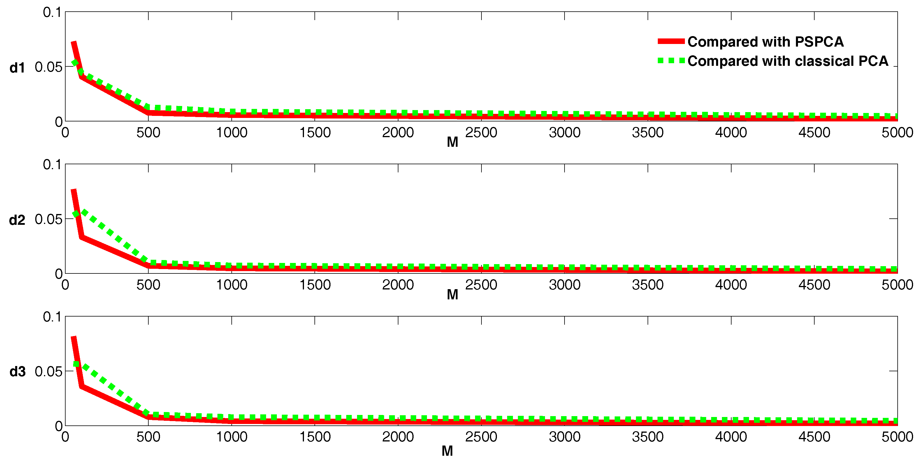
Then, we can compare the performance of our sampling-based histogram PCA method with the single-value benchmark and the PSPCA method with the resulting PCs, as shown in Figure 2.

The solid line shows the Wasserstein distance between ${\mathbf{Y}}_j$ and ${\mathbf{Y}}_j^{PSPCA}$ and the dotted line denotes the Wasserstein distance between ${\mathbf{Y}}_j$ and ${\mathbf{Y}}_j^{NUM}$. The results shown in this figure indicate that the projections of sampling-based histogram PCA, PSPCA, and the single-value benchmarks are generally close. More specifically, the distances decrease as the random sampling size increases during sampling-based projection; when the sample size is more than 1000, the difference is close to zero. These results demonstrate the accuracy of sampling-based histogram PCA projection.

4.3. Example 3

In the third example, we verify the time-saving effects of the multicore MapReduce implementation of the new histogram PCA method. First, we generated observations of the histogram-valued variables ${\mathbf{X}}_k,(k=1\dots p)$. Then, we implemented the method in two different versions: one running MapReduce and the other a serial implementation without the new framework. The execution times of both approaches are compared. Here, we compare results using 1, 2, 4 and 8 cores.

First, we create observations for each histogram-valued variable ${\mathbf{x}}_k$. The simulated symbolic data tables are built as in Examples 1 and 2.

Based on the concept of symbolic variables, to obtain n observations associated with a histogram-valued variable ${\mathbf{X}}_k$, we simulate 5000 real values corresponding to each unit. These values are then organized in histograms that represent the empirical distribution for each unit. In all observations, the widths of the histograms subintervals are the same.

To perform the simulation experiment, symbolic tables that illustrate different situations were created. In this study, a full factorial design is employed, with the following factors:

• Distribution of the microdata that allow histogram generation corresponding to each observation of the variables ${\mathbf{X}}_k(k=1\dots p)$:
  • Uniform distribution:

    $$x_{kj}\sim U({\delta }_1(j),{\delta }_2(j)),{\delta }_1(j)\sim U(-2,0),{\delta }_1(j)\sim U(0,2),j=1,\dots ,n;$$

    (21)
  • Normal distribution:

    $$x_{kj}\sim N(\mu (j),{\sigma }^2(j)),\mu (j)\sim U(0,1),{\sigma }^2(j)\sim U(0,2),j=1,\dots ,n;$$

    (22)
  • Log-Normal distribution:

    $$x_{kj}\sim lnN(\mu (j),{\sigma }^2(j)),$$

    (23)

    $$\mu (j)\sim U(-0.5,0.5),{\sigma }^2(j)\sim U(0.5,1),j=1,\dots ,n;$$
  • Mixture of distributions: Randomly selected from

    $$\{U(1,3),N(1,1),{\chi }^2(1),lnN(0,0.5),-lnN(0,0.5)\}.$$

    (24)
• Number of histogram-valued variables: p = 3; 5.
• Observation size: n = 100; 500; 1000; 3000.

Based on the simulated histogram-valued variables, we conducted the new histogram PCA method in both parallel and serial. The random sampling size from histogram-valued variables in Step 4 is also 5000, the same as the number of real values we began with to simulate histogram-valued variables. Index $C{R}_1$ and $C{R}_2$ are computed using Equation (12) to analyze the behavior of the new histogram PCA method.Moreover, the execution time of both approach are compared to evaluate the speedup effect.

As the conclusion of different situations is almost the same, for the sake of brevity, in this section, we only provide the results for p = 3 and the uniform distribution.

Table 3. Contribution rate of first and second PCs.

p = 3, Uniform	n	${\mathit{CR}}_1$	${\mathit{CR}}_2$
	100	51.19%	24.44%
	500	52.18%	23.92%
	1000	53.10%	23.46%
	3000	53.21%	23.40%

shows the contribution rate of the 1th and 2th PCs. As can be seen from the table, $C{R}_1$ and $C{R}_2$ explain most of the original information contained in the histogram-valued matrix, indicating that the new histogram PCA method performs well.

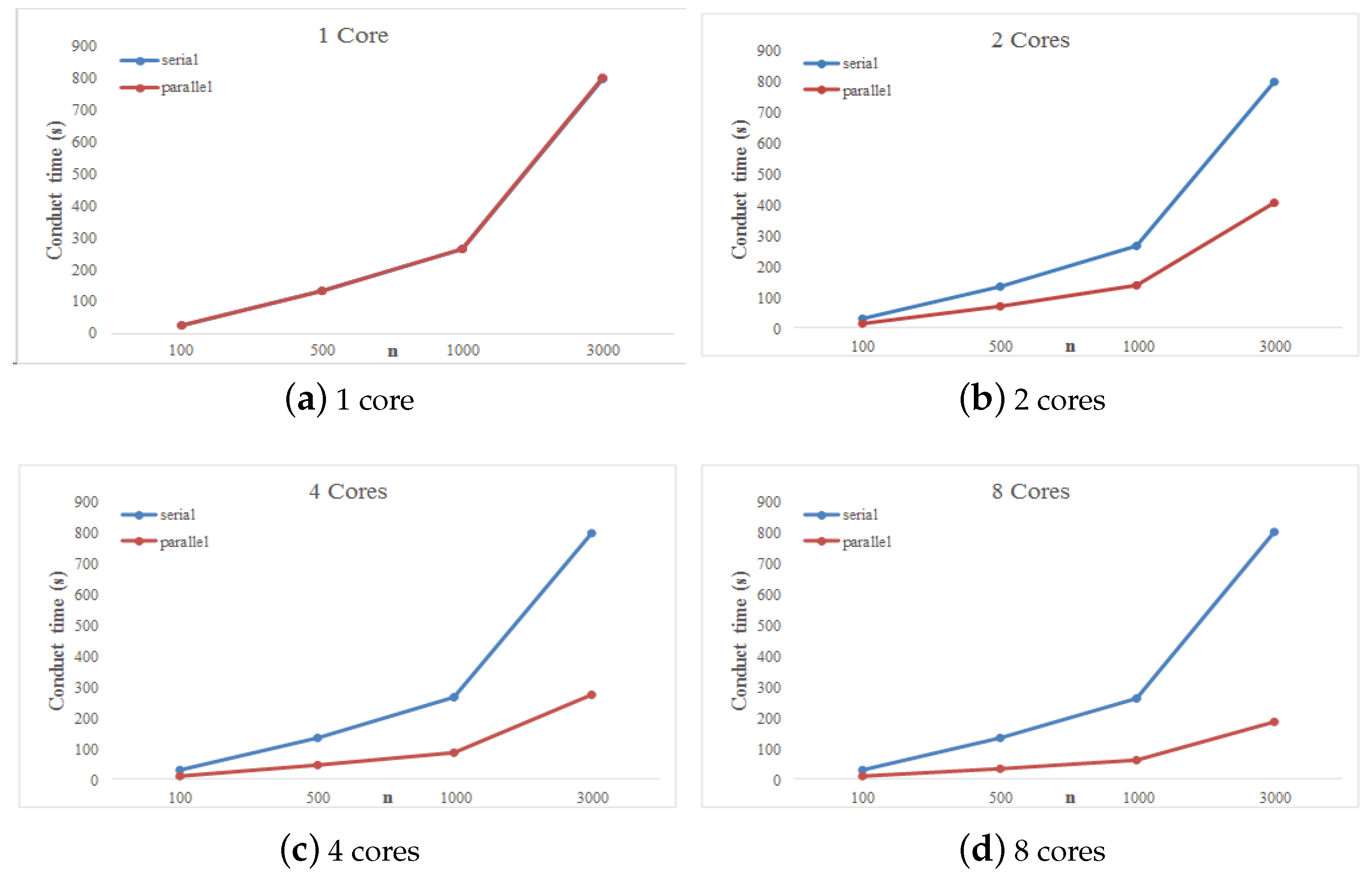
Figure 3 demonstrates the speedup of the method for 1, 2, 4 and 8 processing cores under the MapReduce frame. In Figure 3, we can see that for a given number of cores, execution time increases with sample size. In addition, when sample size is constant, the execution time of the parallel and serial approaches is nearly equivalent when using 1 core. As the number of cores increases, the execution time of the serial approach is essentially unchanged, whereas the execution time of the parallel approach is gradually reduced; the ratio of the execution time between the serial and parallel approaches is nearly the same as the core number. We conclude that the speed increase using a parallel approach with a multicore MapReduce frame is significant.

5. Empirical Study

Nowadays, the rapid development of the Internet has created opportunities for the development of movie sites. The major functions of movie sites are to calculate movie ratings based on user rating data and to then recommend high-quality movies. Since the set of user rating data is massive, symbolic data can be utilized.

In this section, we use real data to evaluate the performance of sampling-based histogram PCA. The data consists of 198,315 ratings from a Chinese movie site from October 2009 to May 2014. The ratings come from three different types of users: visitors, normal registered users, and expert users. In the first step, we summarize movie ratings from the different user types to obtain scoring histograms for each type of user for a movie. Then, the dataset becomes a histogram symbolic table of 500 observations and 3 variables. Finally, sampling-based histogram PCA can be conducted on the generated histogram symbolic table. 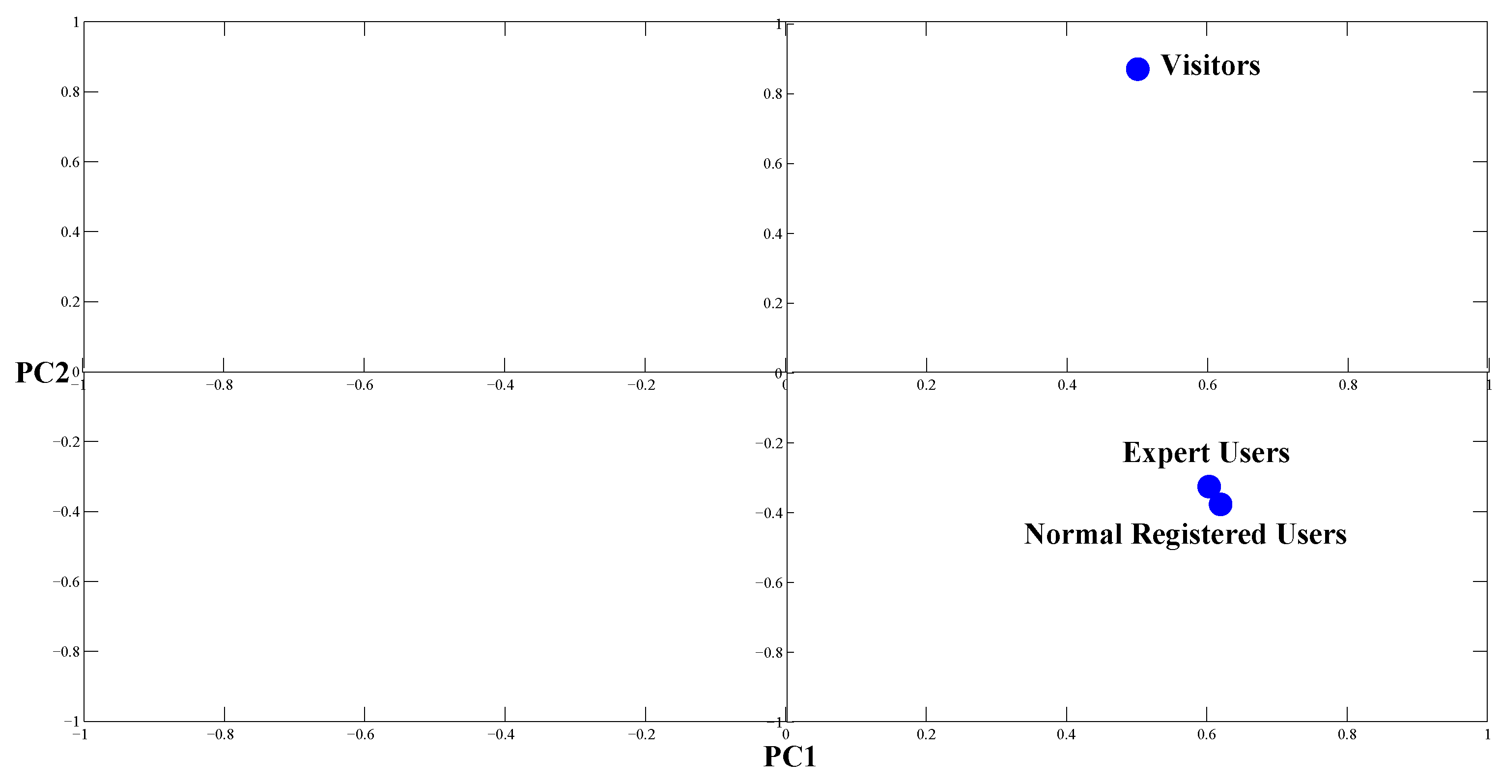We computed the $CR$ index of each PC and show the loading plot of the first and the second PCs in

Table 4. Contribution rate of PCs.

PC	$\mathit{CR}$
$F_1$	73.87%
$F_2$	23.21%
$F_3$	2.92%

and Figure 4.

The results show that the first PC summarizes 73.87% of the total information carried by the original variables. The first PC is positively associated with visitors’, normal registered users’, and expert users’ rating histograms. Thus, we could simply use the first PC as an integrated embodiment of the three types of user ratings, simplifying the evaluation and comparison of different movies.

Next, we verify the performance of the sampling-based projection process using the projection results on the first PC. As the explanatory power of the first PC is very good, if the scores of the first PC can identify the different characteristics of the movies, the projection results are reasonable.

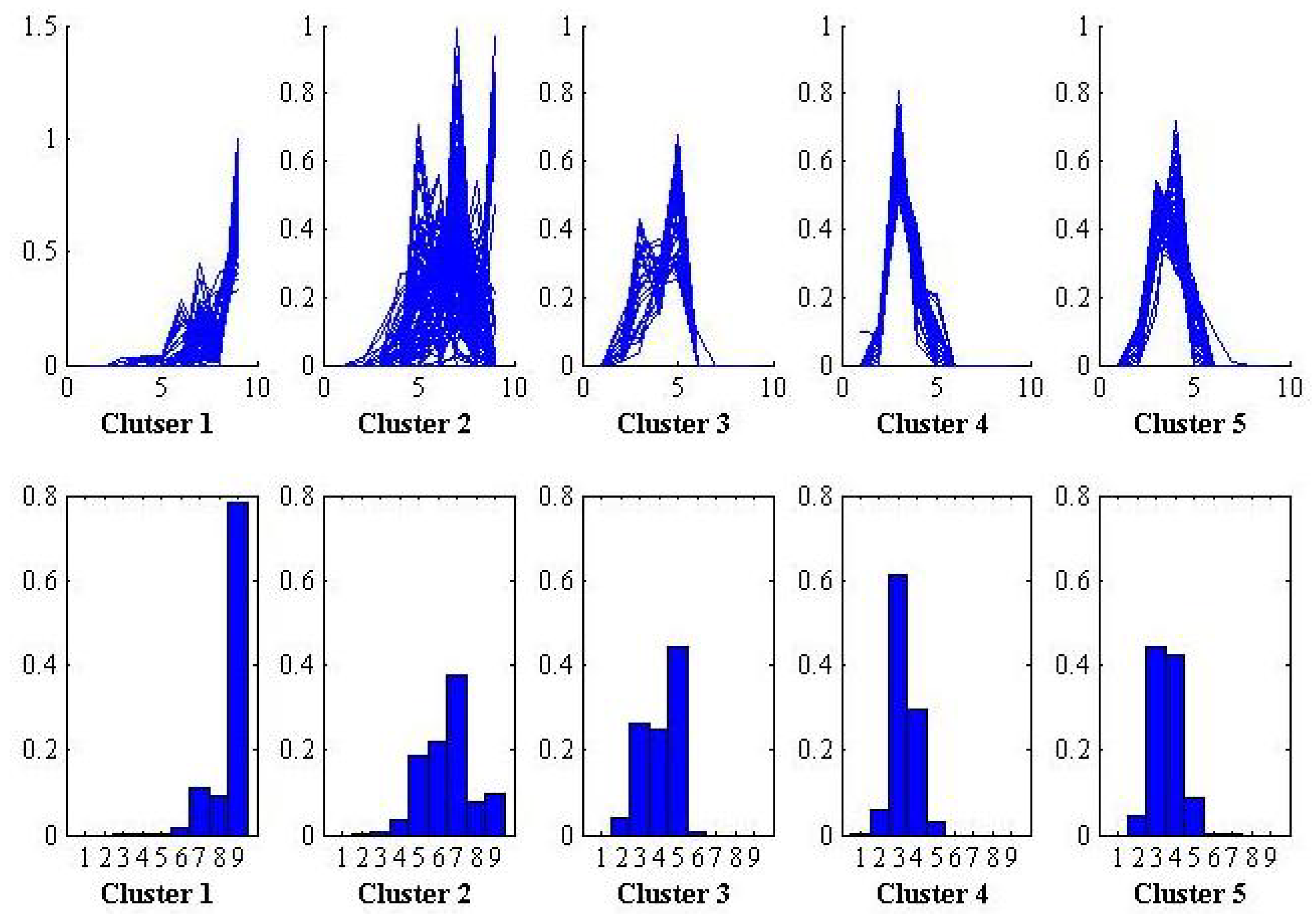
In this empirical study, clustering analysis is implemented on these movies based on the Wasserstein distances [31] between pairs of projections on the first PC and movies are divided into five clusters. During the projection process, we randomly sample 1000 single-value samples from each histogram observation. The projection results of the clusters are showed in Figure 5, where the curves in the first row are the projections of the movies in each cluster. For convenience, we use curve instead of histogram to show the a movie’s scoring probabilities in each score section. The histograms in the second row are the centers of the five clusters in the first row.

The results show that the characteristics of different categories of movie are different. The movies in Cluster 1 receive high ratings; movies in Cluster 2 are distributed relatively equally across score sections; movies in Cluster 3 are distributed relatively equally among low-score sections; and the movies in Clusters 4 and 5 are low grade, mainly distributed in 3 and 3-4 point ratings, respectively.

As can be seen, the final ratings histograms clearly reflect different types of movies, which indicate that the method proposed in this paper performs effectively.

6. Conclusions

As there is no precise, unified method of linear combination of histogram-valued symbolic data, the paper presents a more accurate histogram PCA method, which can project observations onto the space spanned by PCs by random sampling numerical data from the histogram-valued variables. Furthermore, considering that the sampling algorithm is time-consuming and that the sampling can be done separately, we adopt a MapReduce paradigm to implement the new histogram PCA algorithm. A simulation study and an empirical study were performed to analyze the behavior of the new histogram PCA method and to demonstrate the effect of MapReduce parallel implementation. The new method performs well and can be sped up significantly through a multicore MapReduce framework.

In practice, the sampling method for the linear combination of histogram data proposed in the paper can be popularized and applied widely on other multivariable statistical models for histogram data, such as linear regression model, linear discriminant analysis model, and so on. Using sampling method will provide a new perspective for these methods, but further research is needed in the future.