Article

New Holographic Dark Energy Model in Brans-Dicke Theory

1
Department of Mathematics, University of the Punjab, Quaid-e-Azam Campus, Lahore 54590, Pakistan
2
Division of Human Support System, Faculty of Symbiotic Systems Science, Fukushima University, Fukushima 960-1296, Japan
*
Author to whom correspondence should be addressed.
Symmetry 2018, 10(5), 153; https://doi.org/10.3390/sym10050153
Submission received: 17 April 2018 / Revised: 4 May 2018 / Accepted: 4 May 2018 / Published: 11 May 2018
(This article belongs to the Special Issue Cosmological Inflation, Dark Matter and Dark Energy)

Abstract

:
We study the cosmic evolution of the Bianchi type I universe by using new holographic dark energy model in the context of the Brans-Dicke theory for both non-interacting and interacting cases between dark energy and dark matter. We evaluate the equation of state for dark energy ω D and draw the ω D ω ˙ D plane, where the dot denotes the time derivative. It is found that a stage in which the cosmic expansion is accelerating can be realized in both cases. In addition, we investigate the stability of the model by analyzing the sound speed. As a result, it is demonstrated that for both cases, the behavior of the sound speed becomes unstable. Furthermore, with the Om-diagnostic tool, it is shown that the quintessence region of the universe can exist.
PACS:
04.50.kd; 95.36.+x

1. Introduction

In 1961, Brans and Dicke [1] proposed an alternative to General Relativity theory, by absorbing Mach’s principle (which states that inertial forces experienced by a body in non-uniform motion are determined by the distribution of matter in the universe) into gravity, named as Brans-Dicke (BD) theory. In this theory, the dynamic of gravity is represented by a scalar field, while the metric tensor solely incorporates the spacetime structure. As a consequence, gravity couples with a time-dependent scalar field, ψ ( t ) , corresponding to the inverse of Newton’s gravitational constant, G ( t ) , through a coupling parameter ω .
On the other hand, the holographic dark energy (HDE) approach appears to play a fundamental role in cosmic evolution (for recent reviews on the issue of dark energy and the theories of modified gravity, see, for instance, [2,3,4,5,6,7,8]). The holographic principle states that the number of degrees of freedom in a bounded system should be finite and associated to its boundary area. According to this principle, there is a theoretical relation between infrared and ultraviolet cutoffs. This model was originally proposed by Li [9] who used the basic concept of holographic principle in the background of Quantum Gravity. He concluded that, in a system having an ultraviolet cutoff and size L , the total energy should not be more than that of a black hole with the same size, leading to L 3 ρ D L M p 2 (where M p = ( 8 π G e f f ) 1 2 and ρ D represent the reduced Planck mass and the energy density of HDE, respectively). He also investigated three choices of L which are assumed to give an infrared cutoff. First, he assumed L = H 1 introducing the most natural choice for the infrared cutoff in the formalism of HDE, but this choice could not illustrate the accelerated expansion of the universe in General Relativity [10] and BD gravity [11]. As a Second cutoff, the particle horizon radius was selected, which also failed to explain the current cosmic behavior. A future event horizon was the third choice, which eventually managed to yield the desired results. However, in this case, extra care is needed, since future singularities may lead to an undesirable phenomenology of the Universe (see, e.g., [12,13]).
More recently, Granda and Oliveros [14] considered a HDE model in which the energy density depends on the Hubble parameter and its derivative, being referred to as the new holographic dark energy (NHDE) model. Oliveros and Acero [15] studied this NHDE approach in the vicinity of the FRW metric with a non-linear interaction between DE and DM, and discussed the portrait of the equation of state (EoS) parameter ω D , on the ω D ω ˙ D plane, as well as its behavior with the aid of the Om-diagnostic tool. Fayaz et al. [16] investigated HDE model in a Bianchi Type I with (BI) universe within the context of the generalized teleparallel theory and found phantom/quintessence regions of the universe. Sadri and Vakili [17] studied the NHDE approach in BD theory using a FRW universe model with logarithmic scalar field, and analyzed the EoS/deceleration parameter, statefinder and Om-diagnostic tool for both non-interacting/interacting case. Jahromi et al. [18] studied the generalized entropy formalism and used a NHDE model to illustrate the evolution of the universe through its cosmological parameters.
The effects of anisotropy in the universe can be studied in the framework of an anisotropic BI model. Reddy et al. [19] analyzed homogeneous and axially symmetric BI models in BD theory and found that the deceleration parameter is negative, leading to an accelerated expansion of the universe. Setare [20] studied the HDE model with non-flat FRW metric in BD cosmology and found that the EoS parameter demonstrates a phantom-like region and crosses the phantom divide line. Kumar and Singh [21] used exact solutions describing BI cosmological models to study the cosmic evolution in a scalar-tensor theory. Setare and Vanegas [22] investigated an interacting HDE model and discussed cosmological implications. Sharif and Kausar [23,24] examined the dynamical behavior of a Bianchi universe with anisotropic fluid in f ( R ) gravity. Sharif and Waheed [25] studied the evolution of a BI model in BD theory, using isotropic, anisotropic, as well as magnetized anisotropic fluid, and found that the latter may attain isotropy to the universe. Milan and Singh [26] discussed an HDE model with infrared cutoff as a future event horizon, as well as a logarithmic form of BD scalar field for the FRW universe in BD theory. Felegary et al. [27] studied the dynamics of an interacting HDE model in BD cosmology as regards the future event horizon cutoff, as well as its Hubble-horizon counterpart, and discussed the coincidence problem.
In this paper, we consider the NHDE approach for a BI universe and study the associated cosmic evolution in the background of BD theory. It should be noted that the present HDE model under consideration is corresponding to a kind of particular case of the investigations in [28] and its generalized considerations [29]. The outline of the paper is as follows. In Section 2, we study the NHDE model for non-interacting as well as in the interacting case and investigate the associated cosmological parameters. We also analyze the stability of the NHDE model through the corresponding sound speed. Section 3 deals with the Om-diagnostic tool, to study the cosmic evolution. Finally, we summarize our results in Section 4.

2. NHDE Model and BD Theory

The action for the BD theory is [1]
S = d 4 x g ω ψ g i j i ψ j ψ ψ R + L m ,
where R and L m represent the Ricci scalar and matter Lagrangian density, respectively. The field equations for BD theory are
G i j = 1 ψ ( T i j ( m ) + T i j ( ψ ) ) ,
ψ = T ( m ) 2 ω + 3 ,
where
T i j ( m ) = ( ρ + p ) u i u j p g i j , T i j ( ψ ) = ψ , i ; j g i j ψ + ω ψ ( ψ , i ψ , j 1 2 g i j ψ , α ψ , α ) , T ( m ) = g i j T i j ( m ) .
Here, G i j indicates the Einstein tensor, □ is the d’Alembertian operator while T i j ( m ) and T i j ( ψ ) are the energy-momentum tensors for matter distribution and scalar field, respectively. Equations (2) and (3) represent the field equations for BD theory and equation of evolution for the scalar field, respectively. We consider homogeneous and anisotropic locally rotationally symmetric BI universe model as
d s 2 = d t 2 A 2 ( t ) d x 2 B 2 ( t ) ( d y 2 + d z 2 ) ,
where A and B indicate the scale factors in spatial directions.
The corresponding field equations for BI model are
2 A ˙ B ˙ A B + B 2 ˙ B 2 + A ˙ A + 2 B ˙ B ψ ˙ ψ ω 2 ψ 2 ˙ ψ 2 = ρ m + ρ D ψ ,
2 B ¨ B + B 2 ˙ B 2 + ψ ¨ ψ + 2 B ˙ B ψ ˙ ψ + ω 2 ψ 2 ˙ ψ 2 = p D ψ ,
B ¨ B + A ˙ B ˙ A B + A ¨ A + A ˙ A + B ˙ B ψ ˙ ψ + ψ ¨ ψ + ω 2 ψ 2 ˙ ψ 2 = p D ψ ,
where dot represents derivative with respect to t. In the above equations, ρ D and ρ m indicate DE and DM energy densities, respectively, while p D is the pressure of DE. For the scalar field ψ , the wave equation in (3) takes the form
ψ ¨ + A ˙ B + 2 B ˙ B ψ ˙ ρ m + ρ D 3 p D 2 ω + 3 = 0 .
For the sake of simplicity, we take A = B m , m 1 , consequently, Equations (5), (7) and (8) turn out to be
( 2 m + 1 ) B 2 ˙ B 2 + ( m + 2 ) B ˙ B ψ ˙ ψ ω 2 ψ 2 ˙ ψ 2 = ρ m + ρ D ψ ,
( m + 1 ) B ¨ B + m 2 B 2 ˙ B 2 + ( m + 1 ) B ˙ B ψ ˙ ψ + B ˙ B ψ ˙ ψ + ψ ¨ ψ + ω 2 ψ 2 ˙ ψ 2 = p D ψ ,
ψ ¨ + ( m + 2 ) B ˙ B ψ ˙ ρ m + ρ D 3 p D 2 ω + 3 = 0 .
Due to non-linear field equations, we suppose power-law model for the scalar field as ψ ( t ) = ψ 0 B α , α > 0 and ψ 0 are constants. Subtracting Equation (10) from (6) and using power-law relation, we obtain a differential equation for the scale factor B as
B ¨ B + ( m + α + 1 ) B 2 ˙ B 2 = 0 ,
whose integration leads to
B ( t ) = ( m + α + 2 ) 1 m + α + 2 ( c 1 t + c 2 ) 1 m + α + 2 ,
where c 1 and c 2 are integration constants. Consequently, we have
A ( t ) = ( ( m + α + 2 ) ( c 1 t + c 2 ) ) m m + α + 2 .
For our line element, the mean Hubble parameter is given as
H = 1 3 A ˙ A + 2 B ˙ B .
Using A = B m and Equation (12), the above equation yields
H = c 1 ( m + 2 ) ( m + α + 2 ) ( c 1 t + c 2 ) .
In the following, we discuss non-interacting and interacting cases of NHDE and investigate cosmological parameters graphically.

2.1. Non-Interacting Case

In this section, we discuss the case when DE and DM do not interact, the corresponding conservation equations are
ρ ˙ D + 3 ( 1 + ω D ) ρ D H = 0 ,
ρ ˙ m + 3 ρ m H = 0 ,
where ω D = p D ρ D is the EoS parameter through which we analyze different universe eras. The energy density of HDE model is defined as
ρ D = 3 n 2 M p 2 L 2 ,
where n is a dimensionless constant. The energy density of NHDE model is given by
ρ D = 3 n 2 M p 2 L 2 1 ϵ L 3 r c ,
here r c = M p 2 2 M 5 3 is the crossover length scale while ϵ = ± 1 denotes self-accelerated and normal branches of solution. If L 3 r c , the above energy density reduces to the energy density of HDE model. The fractional energy densities in their usual form are given as
Ω m = ρ m ρ c r = 4 ω ρ m 3 ψ 2 H 2 ,
Ω D = ρ D ρ c r = c 2 1 ϵ 3 H r c ,
where r c = 1 2 H Ω r c . Taking time derivative of Equation (16), we obtain
ρ ˙ D = ρ D 2 ψ ˙ ψ + 2 H ˙ H + c 2 ϵ ψ 2 Ω r c H ˙ H 2 ω .
Using Equation (13), we have
H ˙ H 2 = 3 ( m + α + 2 ) m + 2 .
Differentiating Equation (18) with respect to t, we find
Ω ˙ D = 2 3 ϵ c 2 Ω r c H ˙ H .
Using Equations (14) and (19), the EoS parameter turns out to be
ω D = 1 2 α m + 2 + Ω D + c 2 Ω D m + α + 2 m + 2 .
We fix the value of fractional density of DE as Ω D = 0.73 [30] while other parameters are fixed as c = 0.8 , m = 1.55 and α > 0 . Using these values in the above equation, we see that ω D < 0 which corresponds to accelerated behavior of the universe. Caldwell and Linder [31] investigated that the quintessence model of DE can be separated into two distinct regions, i.e., thawing and freezing regions through ω D ω ˙ D plane. The thawing region is characterized when ω ˙ D > 0 , ω D < 0 while the freezing region is determined for ω ˙ D < 0 , ω D < 0 . Taking the time derivative of Equation (21), it follows that
ω ˙ D = 2 3 ϵ Ω r c c 4 c 1 ( m + α + 2 ) Ω D 2 ( c 1 t + c 2 ) ( m + 2 ) .
In this scenario, we plot ω D ω ˙ D plane for two values of integration constant c 2 (Figure 1). The left plot indicates that positive value of c 2 leads to ω ˙ D > 0 , ω D < 0 which corresponds to thawing region. The right graph is plotted for c 2 = 10 showing that negative value of c 2 yields freezing region for NHDE model.
Now, we analyze stability of the NHDE model using squared speed of sound given as
υ s 2 = p ˙ D ρ ˙ D = ω D + ω ˙ D ρ D ρ ˙ D .
The model is unstable for υ s 2 ( t ) < 0 while υ s 2 ( t ) > 0 leads to stability. Using Equations (19), (21) and (22) in (23), it follows that
υ s 2 = 1 2 α m + 2 + Ω D + c 2 Ω D m + α + 2 m + 2 2 ϵ Ω r c c 4 c 1 ( m + α + 2 ) ( ( m + α + 2 ) ( c 1 t + c 2 ) ) 2 α m + α + 2 ( 1 2 3 ϵ Ω r c ) Ω D 2 ( c 1 t + c 2 ) ( m + 2 ) × [ 3 ( ( m + α + 2 ) ( c 1 t + c 2 ) ) 2 α m + α + 2 ( 1 2 3 ϵ Ω r c ) ( 2 α c 1 ( m + α + 2 ) ( c 1 t + c 2 ) 2 c 1 c 1 t + c 2 ) 2 c 1 ϵ ( m + α + 2 ) 2 m + α + 2 3 ( c 1 t + c 2 ) 2 m + α + 4 3 ] 1 .
The graph of υ s 2 ( t ) versus t is shown in Figure 2, where the unit of time t is taken as second. The change in free parameters does not affect the behavior of υ s 2 ( t ) , so we show only one plot here.
It is found that υ s 2 ( t ) < 0 , representing that our model is unstable.

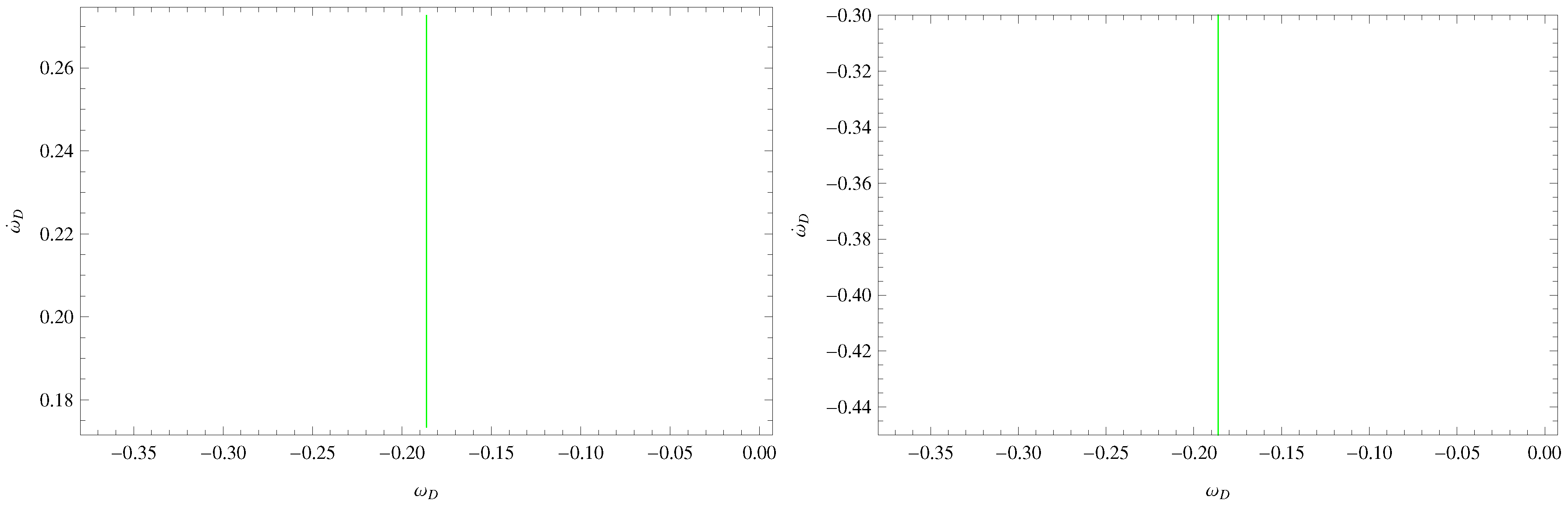
2.2. Interacting Case
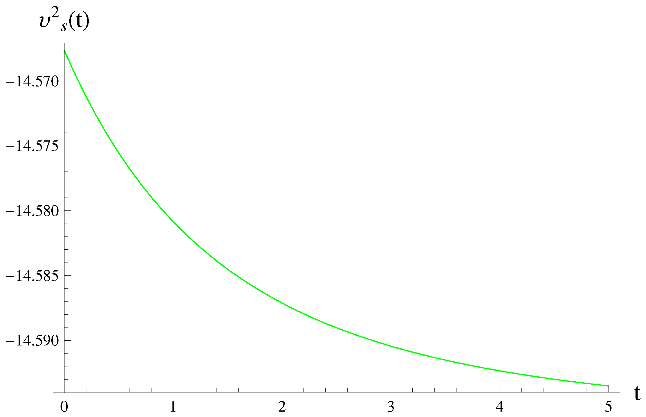
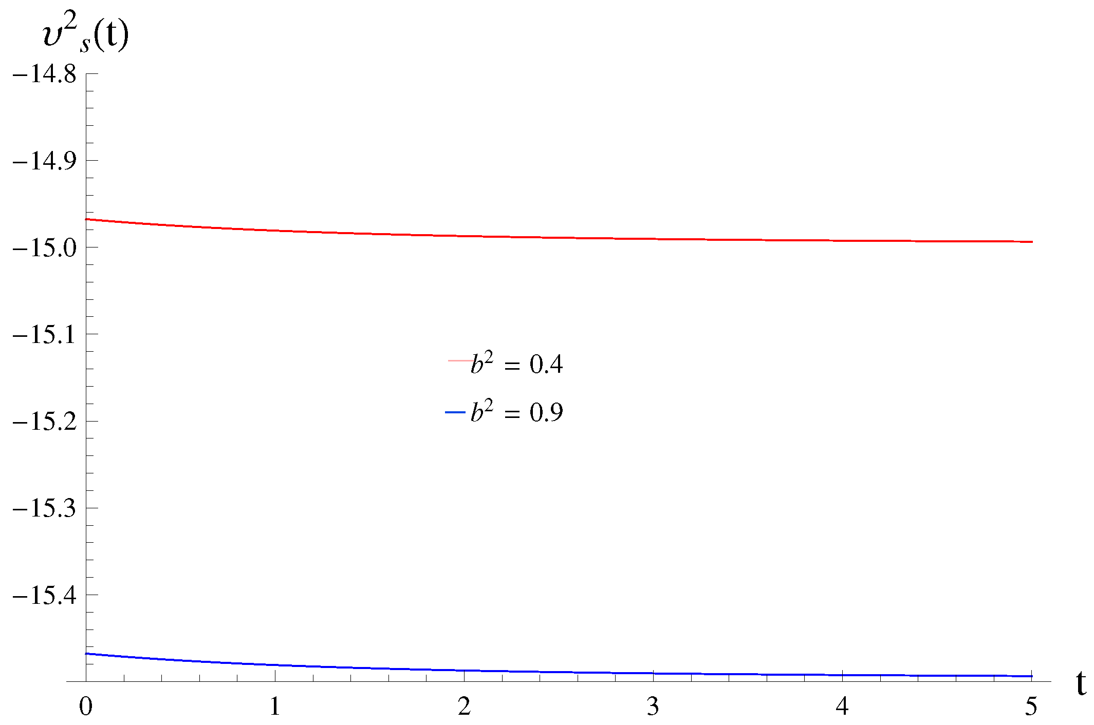
Here we study the case when both dark components, i.e., DM and DE, interact with each other. In this case, the continuity equations are given by
ρ ˙ D + 3 ( 1 + ω D ) ρ D H = Γ ,
ρ ˙ m + 3 ρ m H = Γ ,
where Γ = 3 b 2 H ρ D is a particular interacting term with the interacting parameter b 2 . Using Equations (20) and (25), the EoS parameter is given by
ω D = 1 b 2 2 α m + 2 + Ω D + c 2 Ω D m + α + 2 m + 2 .
In order to observe the behavior of the EoS parameter, we fix the constants Ω D , m , c , α as for the previous case while the interacting parameter will be varied. We observe that ω D exhibits similar behavior as in non-interacting case, i.e., it demonstrates accelerated behavior of the universe. Taking derivative of the above equation with respect to t, we have
ω ˙ D = 2 3 ϵ Ω r c c 4 c 1 ( m + α + 2 ) Ω D 2 ( c 1 t + c 2 ) ( m + 2 ) .
Figure 3 shows the graph of ω D ω ˙ D plane for two values of the interacting parameter. It is found that ω D ω ˙ D plane corresponds to thawing and freezing regions for c 2 = 5 and c 2 = 10 , respectively. Using Equations (19), (27) and (28) in (23), the sound speed parameter takes the form
υ s 2 = 1 b 2 2 α m + 2 + Ω D + c 2 Ω D m + α + 2 m + 2 2 ϵ Ω r c c 4 c 1 ( m + α + 2 ) ( ( m + α + 2 ) ( c 1 t + c 2 ) ) 2 α m + α + 2 ( 1 2 3 ϵ Ω r c ) Ω D 2 ( c 1 t + c 2 ) ( m + 2 ) × [ 3 ( ( m + α + 2 ) ( c 1 t + c 2 ) ) 2 α m + α + 2 ( 1 2 3 ϵ Ω r c ) ( 2 α c 1 ( m + α + 2 ) ( c 1 t + c 2 ) 2 c 1 c 1 t + c 2 ) 2 c 1 ϵ ( m + α + 2 ) 2 m + α + 2 3 ( c 1 t + c 2 ) 2 m + α + 4 3 ] 1 .
The graph of υ s 2 ( t ) versus t is plotted in Figure 4 which shows that υ s 2 ( t ) < 0 demonstrating that our model is not stable. Here, the unit of time t is taken as second.

3. Om-Diagnostic

Here, we study different stages of the universe through the Om-diagnostic tool [32]. This helps to observe the behavior of the DE model and divides it into two sections. The positive values of Om(t) give phantom-like behavior and its negative values correspond to the quintessence region. The Om-diagnostic tool is defined as
O m ( t ) = h 2 ( t ) 1 t 3 1 ,
where h ( t ) = H ( t ) H 0 , H 0 is the Hubble constant. Using Equation (13), the above equation becomes
O m ( t ) = ( m + 2 ) 2 c 1 2 9 H 0 2 ( ( m + α + 2 ) ( c 1 t + c 2 ) ) 2 1 t 3 1 .
We see that the Om-diagnostic tool attains negative values in the range 1.02 t 5 which shows quintessence behavior of the universe (Figure 5, in which the unit of time t is taken as second).

4. Conclusions

In this paper, we investigate the NHDE approach in a BI cosmological model, to discuss the expanding behavior of the universe in the framework of BD theory. For this purpose, the cosmological parameters are evaluated in two scenarios. First, we consider the case where DM and DE do not interact with each other. In this case, the EoS parameter is negative, leading to a universe that experiences accelerated expansion. We have also analyzed its behavior on the ω D ω ˙ D plane, which indicates that our model lies either in the thawing or in the freezing region, corresponding to a positive or a negative value of the associated integration constant, respectively. Furthermore, the stability of the NHDE model is investigated, using the corresponding speed of sound parameter. It is found that this parameter attains negative values, leading to unstable cosmological models.
Second, the interaction between DM and DE is taken into account. In this case, the same parameters as before are formulated yielding that the EoS remains negative for two values of the interaction parameter, b 2 , i.e., our universe is in an expanding phase. It is also found that the ω D ω ˙ D plane analysis demonstrates similar behavior for both values of b 2 , i.e., our model remains in the thawing and freezing regions. Furthermore, we conclude that such a model does not exhibit stable behavior. Finally, cosmological evolution is discussed also with the aid of the Om-diagnostic tool, which, in our case, exhibits quintessence behavior of the universe. It is quite interesting to mention that our results are consistent with the corresponding isotropic universe model [17].

Author Contributions

M.S. and S.A.A.S. have mainly executed mathematical calculations and consdered the constructions of the paper. K.B. has adjusted and edited the paper and suggested the investitations on the subject of Holographic Dark Energy.

Acknowledgments

The work of KB is partially supported by the JSPS KAKENHI Grant Number JP 25800136 and Competitive Research Funds for Fukushima University Faculty (17RI017).

Conflicts of Interest

The authors declare no conflicts of interest.

References

  1. Brans, C.; Dicke, R.H. Mach’s principle and a relativistic theory of gravitation. Phys. Rev. 1961, 124, 925. [Google Scholar] [CrossRef]
  2. Nojiri, S.I.; Odintsov, S.D. Unified cosmic history in modified gravity: From F (R) theory to Lorentz non-invariant models. Phys. Rep. 2011, 505, 59–144. [Google Scholar] [CrossRef]
  3. Capozziello, S.; De Laurentis, M. Extended theories of gravity. Phys. Rep. 2011, 509, 167–321. [Google Scholar] [CrossRef]
  4. Nojiri, S.; Odintsov, S.D.; Oikonomou, V.K. Modified gravity theories on a nutshell: Inflation, bounce and late-time evolution. Phys. Rep. 2017, 692, 1–104. [Google Scholar] [CrossRef]
  5. Capozziello, S.; Faraoni, V. Beyond Einstein gravity: A Survey of gravitational theories for cosmology and astrophysics. Fundam. Theor. Phys. 2010, 170. [Google Scholar] [CrossRef]
  6. Bamba, K.; Odintsov, S.D. Inflationary cosmology in modified gravity theories. Symmetry 2015, 7, 220–240. [Google Scholar] [CrossRef]
  7. Bamba, K.; Capozziello, S.; Nojiri, S.I.; Odintsov, S.D. Dark energy cosmology: The equivalent description via different theoretical models and cosmography tests. Astrophys. Space Sci. 2012, 342, 155–228. [Google Scholar] [CrossRef]
  8. Kleidis, K.; Spyrou, N.K. Dark Energy: The Shadowy Reflection of Dark Matter? Entropy 2016, 18, 94. [Google Scholar] [CrossRef]
  9. Li, M. A model of holographic dark energy. Phys. Lett. B 2004, 603, 1–5. [Google Scholar] [CrossRef]
  10. Hsu, SD. Entropy bounds and dark energy. Phys. Lett. B 2004, 594, 13–16. [Google Scholar] [CrossRef]
  11. Xu, L.; Li, W.; Lu, J. Holographic dark energy in Brans–Dicke theory. Eur. Phys. J. C 2009, 60, 135–140. [Google Scholar] [CrossRef]
  12. Nojiri, S.I.; Odintsov, S.D.; Tsujikawa, S. Properties of singularities in the (phantom) dark energy universe. Phys. Rev. D 2005, 71. [Google Scholar] [CrossRef]
  13. Kleidis, K.; Oikonomou, V.K. Effects of finite-time singularities on gravitational waves. Astrophys. Space Sci. 2016, 361, 326. [Google Scholar] [CrossRef]
  14. Granda, L.N.; Oliveros, A. Infrared cut-off proposal for the holographic density. Phys. Lett. B 2008, 669, 275–277. [Google Scholar] [CrossRef]
  15. Oliveros, A.; Acero, M.A. New holographic dark energy model with non-linear interaction. Astrophys. Space Sci. 2015, 357, 12. [Google Scholar] [CrossRef]
  16. Fayaz, V.; Hossienkhani, H.; Pasqua, A.; Amirabadi, M.; Ganji, M. f (T) theories from holographic dark energy models within Bianchi type I universe. Eur. Phys. J. Plus 2015, 130, 28. [Google Scholar] [CrossRef]
  17. Sadri, E.; Vakili, B. A new holographic dark energy model in Brans-Dicke theory with logarithmic scalar field. Astrophys. Space Sci. 2018, 363, 13. [Google Scholar] [CrossRef]
  18. Jahromi, A.S.; Moosavi, S.A.; Moradpour, H.; Graça, J.M.; Lobo, I.P.; Salako, I.G.; Jawad, A. Generalized entropy formalism and a new holographic dark energy model. Phys. Lett. B 2018, 780, 21–24. [Google Scholar] [CrossRef]
  19. Reddy, D.R.; Naidu, R.L.; Rao, V.U. A cosmological model with negative constant deceleration parameter in Brans-Dicke theory. Int. J. Theor. Phys. 2007, 46, 1443–1448. [Google Scholar] [CrossRef]
  20. Setare, M.R. The holographic dark energy in non-flat Brans–Dicke cosmology. Phys. Lett. B 2007, 644, 99–103. [Google Scholar] [CrossRef]
  21. Kumar, S.; Singh, C.P. Exact bianchi type-I cosmological models in a scalar-tensor theory. Int. J. Theor. Phys. 2008, 47, 1722–1730. [Google Scholar] [CrossRef]
  22. Setare, M.R.; Vagenas, E.C. The cosmological dynamics of interacting holographic dark energy model. Int. J. Mod. Phys. D 2009, 18, 147–157. [Google Scholar] [CrossRef]
  23. Sharif, M.; Kausar, H.R. Anisotropic fluid and Bianchi type III model in f (R) gravity. Phys. Lett. B 2011, 697, 1–6. [Google Scholar] [CrossRef]
  24. Sharif, M.; Kausar, H.R. Non-vacuum solutions of Bianchi type VI 0 universe in f (R) gravity. Astrophys. Space Sci. 2011, 332, 463–471. [Google Scholar] [CrossRef]
  25. Sharif, M.; Waheed, S. Anisotropic universe models in Brans–Dicke theory. Eur. Phys. J. C 2012, 72, 1876. [Google Scholar] [CrossRef]
  26. Srivastava, M.; Singh, C.P. Holographic Dark Energy Model in Brans-Dicke Theory with Future Event Horizon. arXiv, 2017; arXiv:1706.06777. [Google Scholar]
  27. Felegary, F.; Darabi, F.; Setare, M.R. Interacting holographic dark energy model in Brans–Dicke cosmology and coincidence problem. Int. J. Mod. Phys. D 2018, 27, 1850017. [Google Scholar] [CrossRef]
  28. Nojiri, S.I.; Odintsov, S.D. Unifying phantom inflation with late-time acceleration: Scalar phantom–non-phantom transition model and generalized holographic dark energy. Gen. Relativ. Gravit. 2006, 38, 1285–1304. [Google Scholar] [CrossRef]
  29. Nojiri, S.I.; Odintsov, S.D. Covariant generalized holographic dark energy and accelerating universe. Eur. Phys. J. C 2017, 77, 528. [Google Scholar] [CrossRef]
  30. Sharif, M.; Jawad, A. Analysis of pilgrim dark energy models. Eur. Phys. J. C 2013, 73. [Google Scholar] [CrossRef]
  31. Caldwell, R.R.; Linder, E.V. Limits of quintessence. Phys. Rev. Lett. 2005, 95. [Google Scholar] [CrossRef] [PubMed]
  32. Sahni, V.; Shafieloo, A.; Starobinsky, A.A. Two new diagnostics of dark energy. Phys. Rev. D 2008, 78. [Google Scholar] [CrossRef]
Figure 1. Plot of ω D ω ˙ D plane with c 2 = 5 (left), c 2 = 10 (right), c 1 = 1 , c = 0.8 , m = 1.55 and α = 3.5 for non-interacting case.
Symmetry 10 00153 g001
Figure 2. Plot of υ s 2 ( t ) versus t (the unit of which is second) with c 1 = 1 , c 2 = 5 , c = 0.8 , m = 1.55 and α = 3.5 for non-interacting case.
Symmetry 10 00153 g002
Figure 3. Plot of ω D ω ˙ D plane with c 2 = 5 (left), c 2 = 10 (right), c 1 = 1 , c = 0.8 , m = 1.55 and α = 3.5 for interacting case.
Symmetry 10 00153 g003
Figure 4. Plot of υ s 2 ( t ) versus t (the unit of which is second) with c 1 = 1 , c 2 = 5 , c = 0.8 , m = 1.55 and α = 3.5 for interacting case.
Symmetry 10 00153 g004
Figure 5. Plot of Om(t) versus t (the unit of which is second) with c 1 = 1 , c 2 = 5 , m = 1.55 , α = 3.5 and H 0 = 68 .
Symmetry 10 00153 g005

