1. Introduction
Material transport problems with phase change are conveniently modelled by Stefan free boundary conditions, in which there is assumed to be a moving sharp interface between phases. In practice, the interface of solidification may consist of a “mushy” zone, within which there is dendritic infiltration of one phase by another. Similarly, crystal dislocations may migrate between one solid crystal phase and another through a region of crystal overlap that may be significant at the microscale (e.g., [
1]). Observable transition zones with two-phase mixtures may occur in environments wherein the temperature varies little from its critical value. For multi-phase dynamical modelling, the next level of realism beyond sharp interfaces is the phase field theory, in which a continuously varying scalar field
interpolates Phase 1 (
) and Phase 0 (
).
is a monotonic function of the concentration of Phase 1. It may be regarded as a surrogate for the relative concentration of one phase. As in most continuum representations of mixtures, after averaging over a representative elementary volume that is large compared to individual particles such as microscopic dendrites, quantities such as density and phase concentration that are discontinuous at the microscale are represented as smoothly varying functions. The concept of the phase variable is a mathematical generalisation of the older concept of a physically measurable order parameter [
2]. The classic example is the magnetisation of a ferromagnetic material. Only since the 1940s have we been able to calculate the critical temperature for the simplest phase transition, which is the magnetisation of the spatially uniform two-dimensional Ising ferromagnet. In practice, phase transitions are not instantaneous and during the transition, the phase structure of a material will be heterogeneous at the microscale. The scalar field theory of a single phase variable, while being a relatively simple model, will still predict some spatially non-uniform phase structures through a transition zone. The transition zone is often referred to as the “mushy” zone, following the analogy of a two-phase water–ice mixture. The morphology of the transition zone is a major determinant of the physical properties of alloys (e.g., [
3]). The Cahn and Hilliard phase field model of phase separation [
4] showed why the transition zone is stable only at length scales below a small characteristic value. Following the works by Allen and Cahn [
5], and by Cahn and Hilliard [
4], phase field theories have been studied for several decades [
6,
7,
8,
9,
10].
The core of usual simplified versions of Allen–Cahn (or of Ginzburg–Landau [
11]) is an equation for direct relaxation to the minima of a double-well potential. The resulting partial differential equation (PDE) is a standard reaction–diffusion equation of the Fitzhugh–Nagumo type,
where
and
s are constants. Here, the two stable steady states are the pure phases
and
. Without a loss of generality,
; otherwise we could interchange the labels of the two phases. The cubic source term drives the dynamics towards bi-stable fixed points, with the zones of attraction separated by the unstable fixed-point at
. The diffusion term allows for forward transport of existing Phase 1 material through the mixture, opposite to the direction of its own concentration gradient. Equivalently, Phase 0 diffuses in the opposite direction, counter to the direction of its own complementary concentration gradient. Note also that the cubic source term has also appeared in the context of population genetics, as a correct modification to Fisher’s equation for gene frequencies when the genes are not Mendelian but are neither fully dominant nor fully recessive [
12,
13,
14].
The usual simplified Cahn–Hilliard equation is:
The operator is the Laplacian and is the biharmonic operator. The negative Laplacian term (with b < 0) is destabilising, and generates time-reversed diffusion. It has positive spectrum, with amplification of perturbations at high spatial frequency. However, when the spatial frequency is high enough, the instability is restrained by an opposing negative biharmonic term (with a < 0) which has a negative spectrum, and at high spatial frequencies, the overall spectral values are negative rather than positive.
Although these diffusion equations do not minimise any action functional, they do result ultimately from an energy functional. In the Cahn–Hilliard approach, the phase flux is the negative gradient of a chemical potential multiplied by a conductivity (e.g., [
4,
6,
9,
15,
16]). The chemical potential
is the variational derivative
, where
is the energy functional. Further, it is reasonable to include within
a component of strain energy
that depends locally on the phase field value as well as on its squared gradient. Karali and Katsoulakis [
16] showed that in some cases, a combined Allen–Cahn–Hilliard equation could indeed be derived from an energy principle, allowing for both a gradient flow and a reaction term that allows for relaxation towards equilibrium:
Comparatively few exact solutions are known for time-dependent multi-dimensional fourth-order nonlinear reaction–diffusion equations. Galaktionov and Svirshchevskii (Example 6.72 of [
17]) constructed some solutions for the thin film equation with the absorption term
, allowing for
simply to be quadratic in Cartesian coordinates
. These solutions, along with a number of others, were derived by Cherniha and Myroniuk [
18] in a comprehensive Lie symmetry classification. In the current article, some more realistic explicit solutions with meaningful boundary conditions will be constructed after a reduction by a strictly nonclassical symmetry. The solutions have nontrivial spatial structure but they approach the pure phase
, exponentially in time.
In
Section 2, we show that a nonclassical symmetry allows one to separate variables to linear equations in space and time, when the nonlinear reaction and diffusivity obey a single relationship. This allows us, in
Section 3, to construct solutions that approach the phase
asymptotically in time when the Allen–Cahn source term is exactly the cubic function that was given in [
5].
In
Section 4, we show how these fourth-order reaction–diffusion equations relate to an energy principle for a flux potential variable that is the analogue of the matrix flux potential that is well-known from nonlinear porous media studies [
19,
20].
In
Section 5, we conclude with a discussion of the solutions, and some open problems.
3. Interior Solutions for Slabs, Cylinders, and Spheres
In order to gain some understanding of the nature of the solutions, we consider interior solutions for slabs, cylinders, and spheres in dimensions , and 3 respectively. The four independent solutions will be trigonometric and hyperbolic functions (), Bessel and modified Bessel (), and spherical Bessel and modified spherical Bessel functions (). The solutions decrease uniformly in t towards . Even if the initial condition has in some significant sub-domain, the region where the source term is tends to stabilise phase .
Therefore, this global approach to Phase 0 should be controlled by the boundary conditions which may include, for example, ideal contact with the exterior pure phase at , or a Robin boundary condition for extraction of Phase 1.
The Case: .
In general coordinate systems with our adopted dimensionless variables, the simplified form of Equation (
14) factorizes as:
where:
For radial flow within the ball
, the Laplacian operator within (
25) is
. The two operator factors commute so (
25) reduces simply to a system of two alternative second-order Helmholtz equations. The general solution
of (
25) in one, two, and three dimensions, with four free parameters
, is:
Here, the spherical Bessel functions are defined simply as , , and .
For radial flows, the flux density of Phase 1 is:
For all values of
n we impose zero flux at
. For
, considering the asymptotic behaviour of
as
shows that
imposes two conditions on
and
:
These admit no non-trivial solutions, so . For alternatively imposing either or also gives two conditions on and similar to those above, which also imply .
For
, imposing
only implies a single condition:
However,
is unbounded and hence unphysical in this context, unless:
which also ensures that
. Again, the above two equations only admit the trivial solution
.
For
,
only implies the condition:
As
is finite, the
case does admit physical solutions where
and
. We can eliminate this extra degree of freedom by imposing
, to match the admissible solutions discussed above for
and
. This gives an extra condition on
and
:
so that again only
is possible.
The boundary
is in contact with pure Phase 0. Imposing
, implies:
We have found in examples that the zero-flux boundary condition at
will result in an inadmissible solution that is not positive semi-definite. However there is a solution that connects smoothly with an external slab of Phase 0, beginning at the boundary
. Assuming
, we deduce:
This has a sequence of solutions for
. With
, the first of these are
and
for
, and 3 respectively, showing an significant increase with dimensionality. Higher values in the sequence of solutions for
are found to produce unphysical solutions exhibiting negative values of
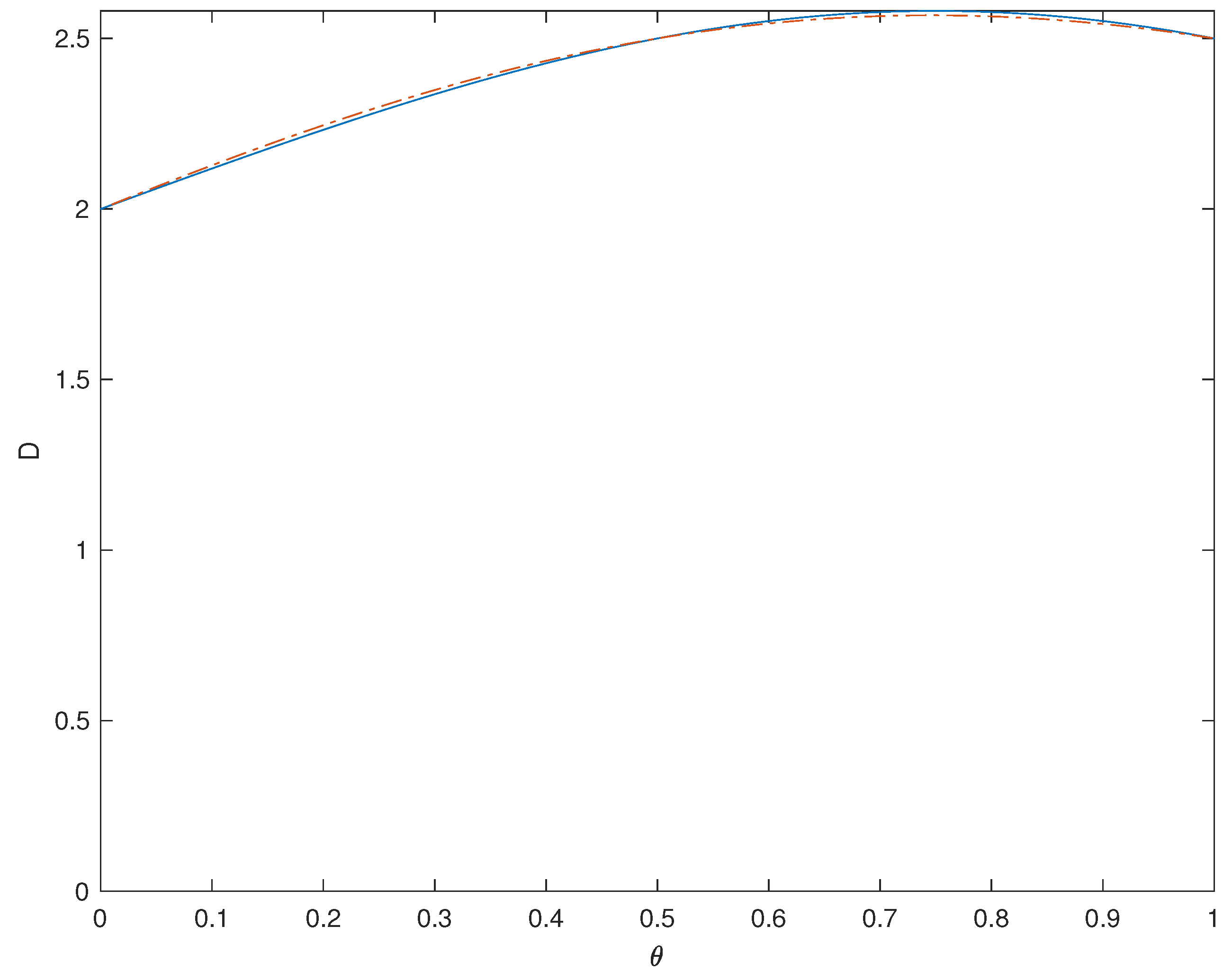
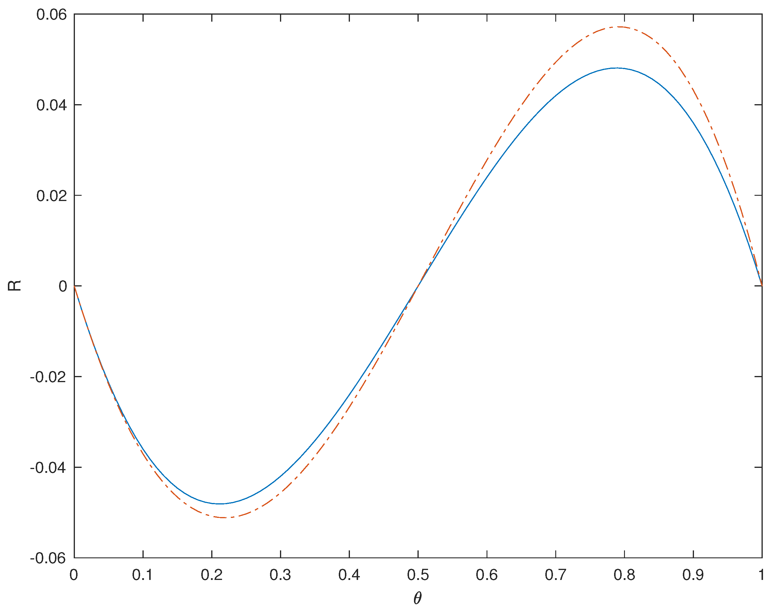
u. With diffusivity
and reaction term
shown in
Figure 1 and
Figure 2 respectively,
is given explicitly in terms of
u as:
Although solutions for
at different times are geometrically similar, this is not true for
which is related to
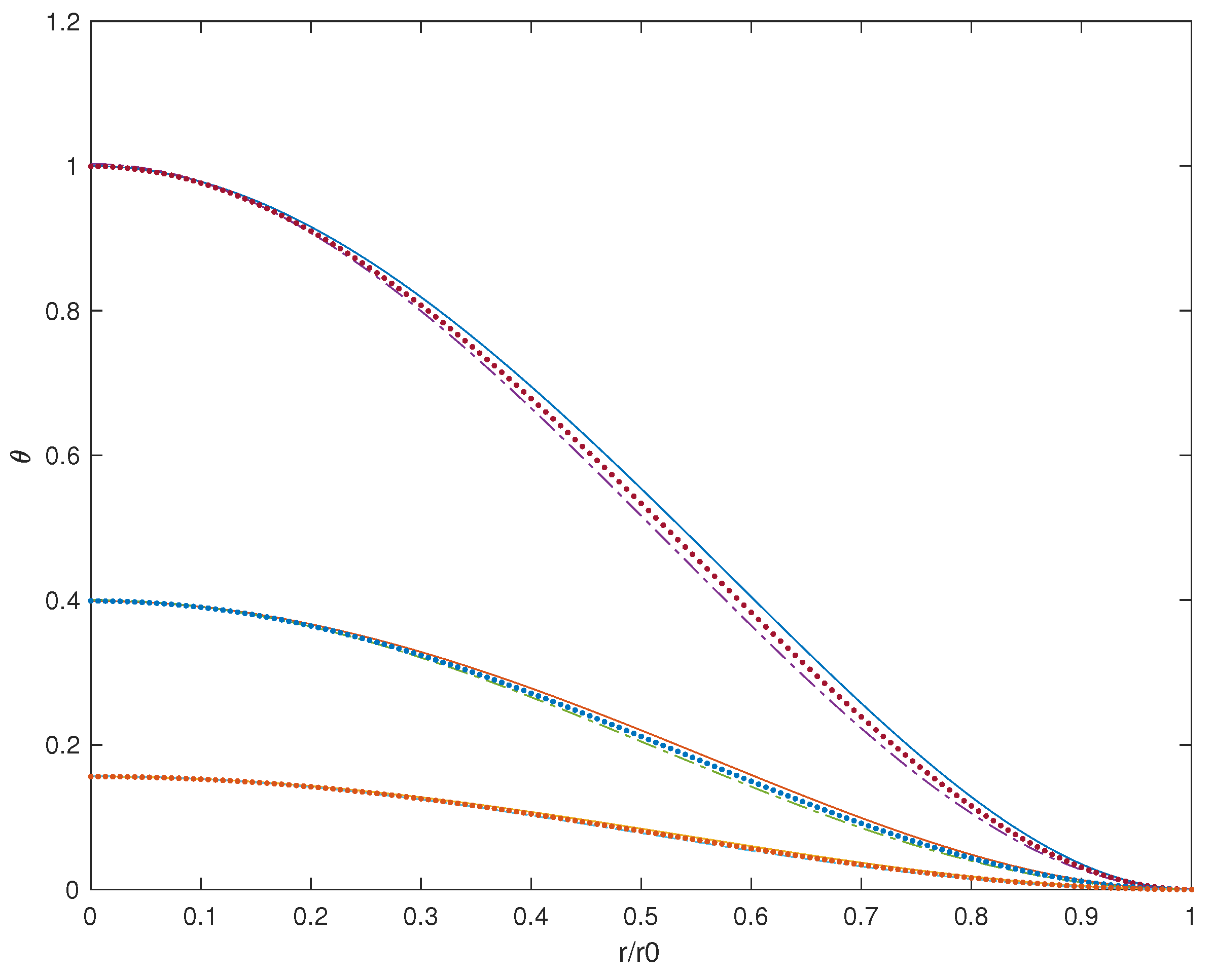
u by a nonlinear transformation. The solution for
is depicted in
Figure 3 for
,
. The solutions in dimensions
are close after the three different domain radii
are rescaled to the same value. The solutions depict an initial region in the neighbourhood of the origin, that consists predominantly of Phase 1, but is connected continuously through a thin mushy zone to a surrounding block of Phase 0, at
. This mushy region is small enough to be stable under the Cahn–Hilliard evolution. Under the influence of the reaction, Phase 1 is normally stable, but its decay in this case is driven by the boundary conditions at
, a boundary where the phase mixture is connected smoothly to an exterior bank of Phase 0. For example, from
to
, the exact radial solution on the interior of the sphere, depicted in
Figure 3, has 90% of the initial volume of Phase 1 material exiting through the boundary, while the remainder undergoes a change to Phase 0 within the interior.
Unphysical solutions, with negative values of
u, were found above for large values of
. If one attempts to find the largest possible value of
that produces a non-negative solution for a given
, it soon becomes clear that for the class of solutions considered above, this corresponds to the first non-zero solution
, of the above conditions
shown in (
33). This is a consequence of our solutions being a linear combination of one oscillatory, and one monotonically increasing function that take finite values at
. As such,
Figure 3 shows scaled examples of solutions with the maximum possible value of
. Selecting smaller values of
produces solutions with a non-zero negative slope at
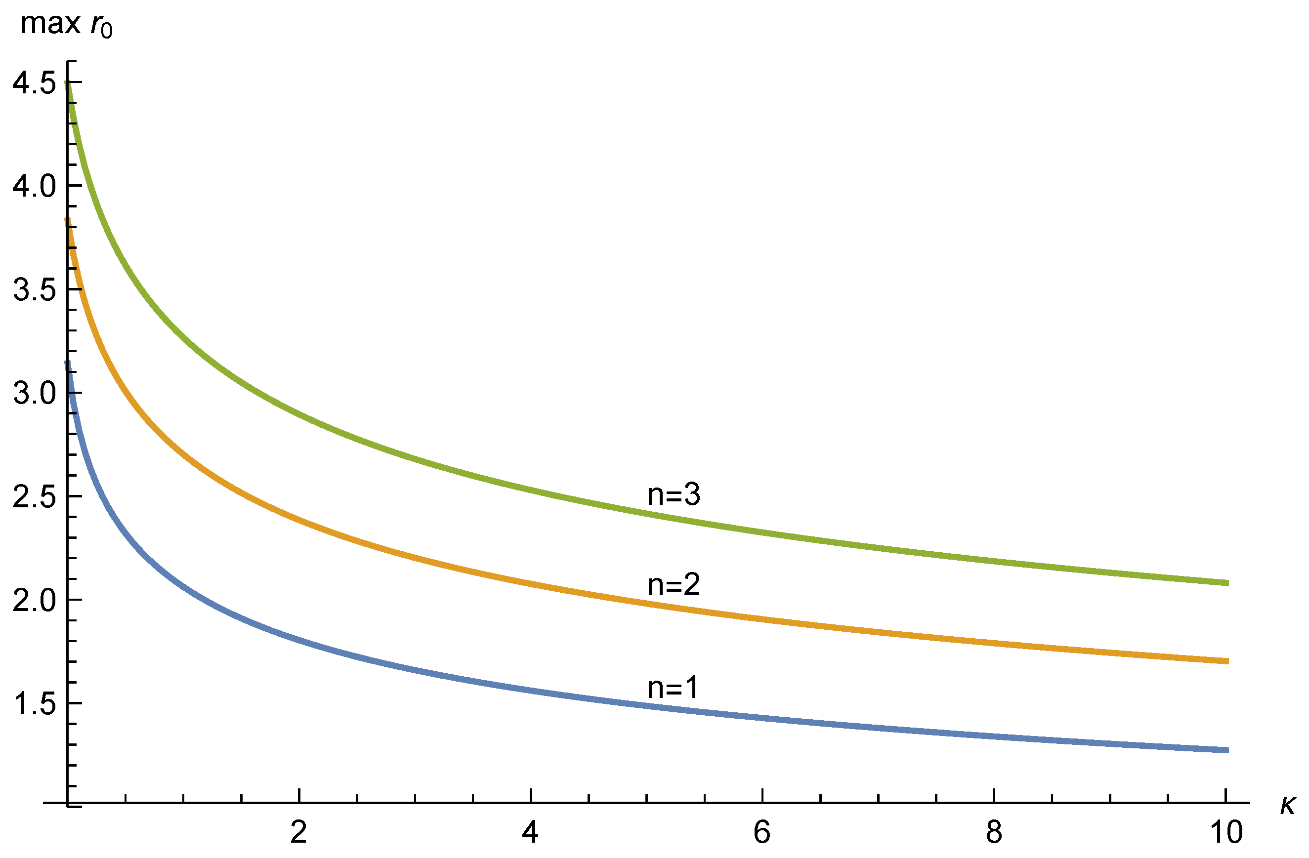
.
Figure 4 shows variation of the maximum possible
value as
varies. In all cases
as
. The case
does not produce valid solutions via our methods above, however the largest possible values of
are obtained as
, and Equation (
33) approaches the following simple conditions in one, two, and three dimensions respectively:
4. Interior Solutions for Rectangular Domains
Under idealised controlled boundary conditions on simple slab, cylindrical, or spherical domains, gives a maximum achievable diameter of the transition zone. However, there are many other solutions with finer sub-structure. This is consistent with the Cahn–Hilliard critical wavelength being of order 1, in dimensionless terms. The initial condition for may be any positive solution of the linear fourth order Helmholtz equation.
If we adopt Cartesian coordinates and restrict our attention to solutions that are identically zero on the boundaries
,
, the dimensionless form of Equation (
14) with
can be solved via the separation of variables. Setting
we find two families of solutions where either:
If we focus on the latter case, and impose
we find compatible values of
:
Meanwhile
must satisfy the differential equation:
provided that
. This produces a solution similar to the first of (
27):
The second form of
above has the boundary condition
imposed. Note that there is a maximum possible value of
that will produce a non-negative
function—hence, the situation is qualitatively similar to the examples of
in various dimensions discussed in
Section 3.
On the other hand, when
we can define:
The corresponding solution
then loses all periodicity:
The above form of
will apply for all
if:
that is, if
is sufficiently small. When this condition is met there is no restriction on the size of
implied by needing a non-negative solution
.
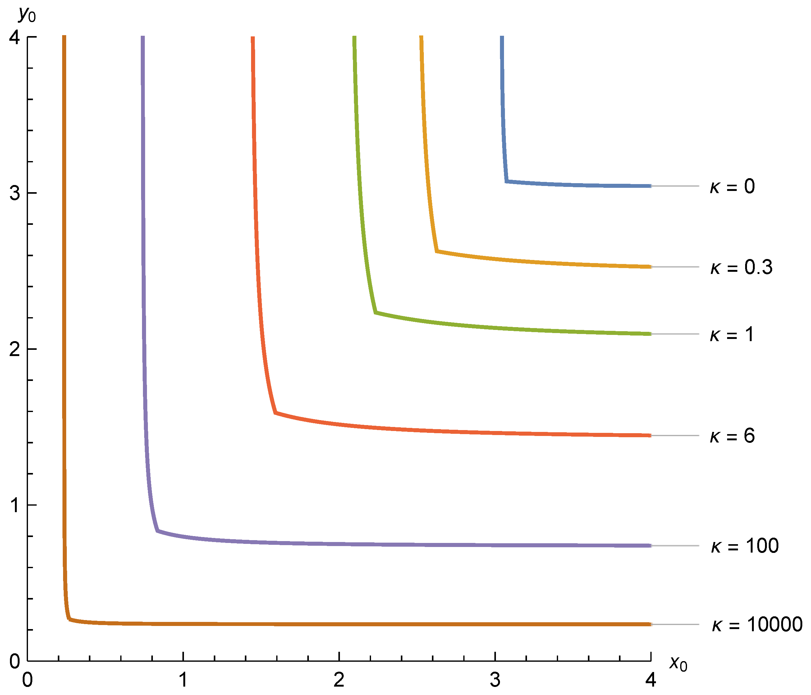
In summary, if
is sufficiently small we can choose
to be as large as we want, however if
shown above, there is some upper limit to the size of
that will produce valid solutions. When all separable modes are accounted for, we can calculate the boundary separating feasible combinations of
and
from infeasible combinations.
Figure 5 illustrates this boundary for various values of
. Note that as
the critical values of
approach those indicated by the
curve of
Figure 4.
When considering combinations of and that admit physical solutions, the eigenvalue corresponding to with = 0 is of primary importance as both and are non-negative. We view solutions with finer substructure as alterations of this solution that maintain the non-negativity of .
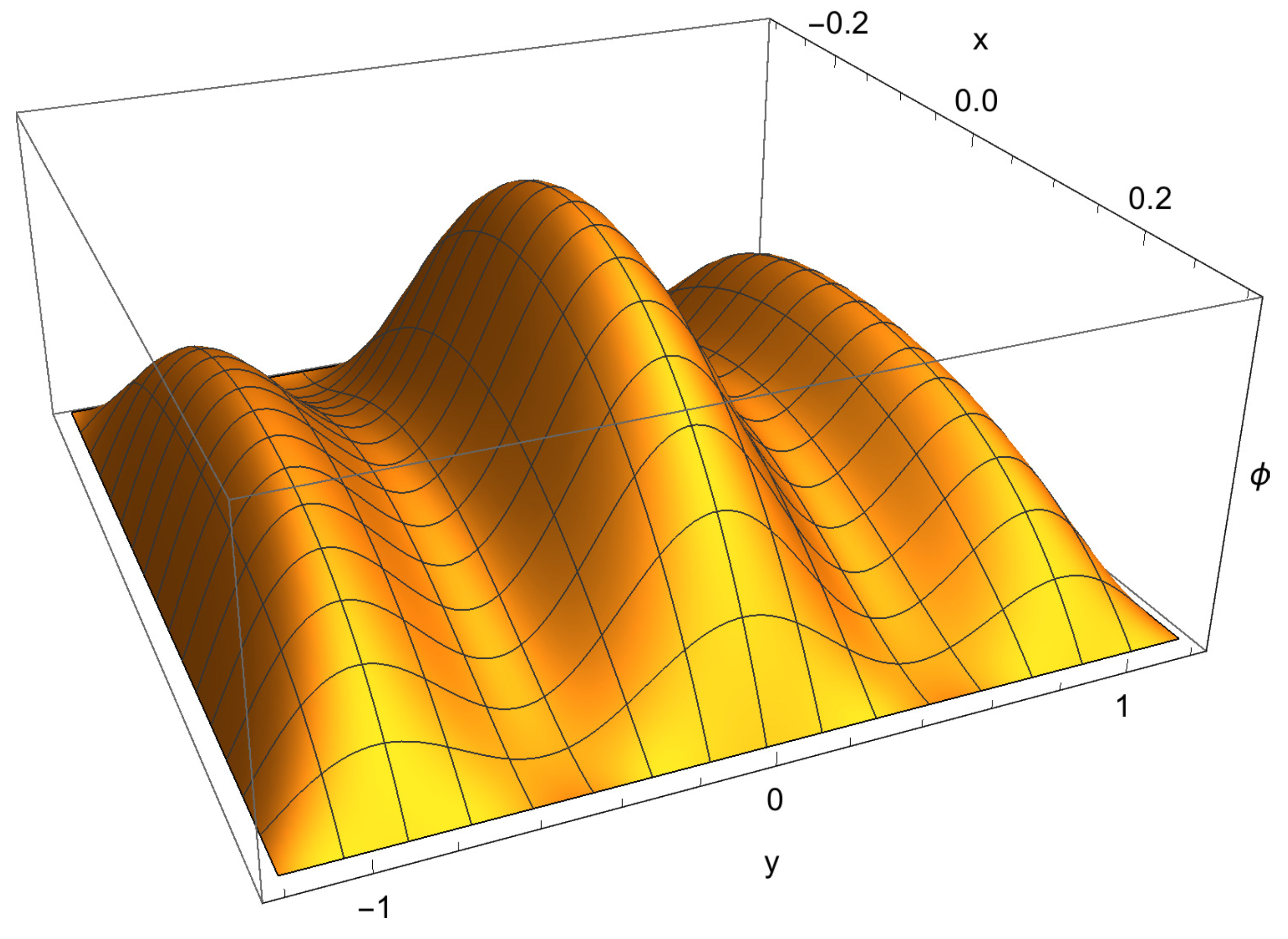
An example with a pronounced sub-structure is shown in
Figure 6. Here,
,
,
, and
is proportional to
where:
From a brief exploration of the parameter space, it appears that solution regions with aspect ratios close to 1 typically allow little variation from
, and tend to be unimodal. Solution regions that are more elongated can be multi-modal, and allow noticeable sub-structure as in the example of
Figure 6.
We can also consider rectangular solutions that are unbounded in a single direction, similar to the one-dimensional solution of
Section 3. Let us begin by assuming that boundary conditions
are applied to Equation (
38) for
. The eigenvalues of
are still restricted by requiring a non-negative solution that remains finite as
. Hence the separable solution must include
,
as its foundation. Equation (40) then gives a non-negative
, provided that
is not larger than the critical values illustrated in
Figure 4 for
. For values of
significantly less than these critical values, we can produce noticeable sub-structure by adding other modes to this base solution while ensuring that
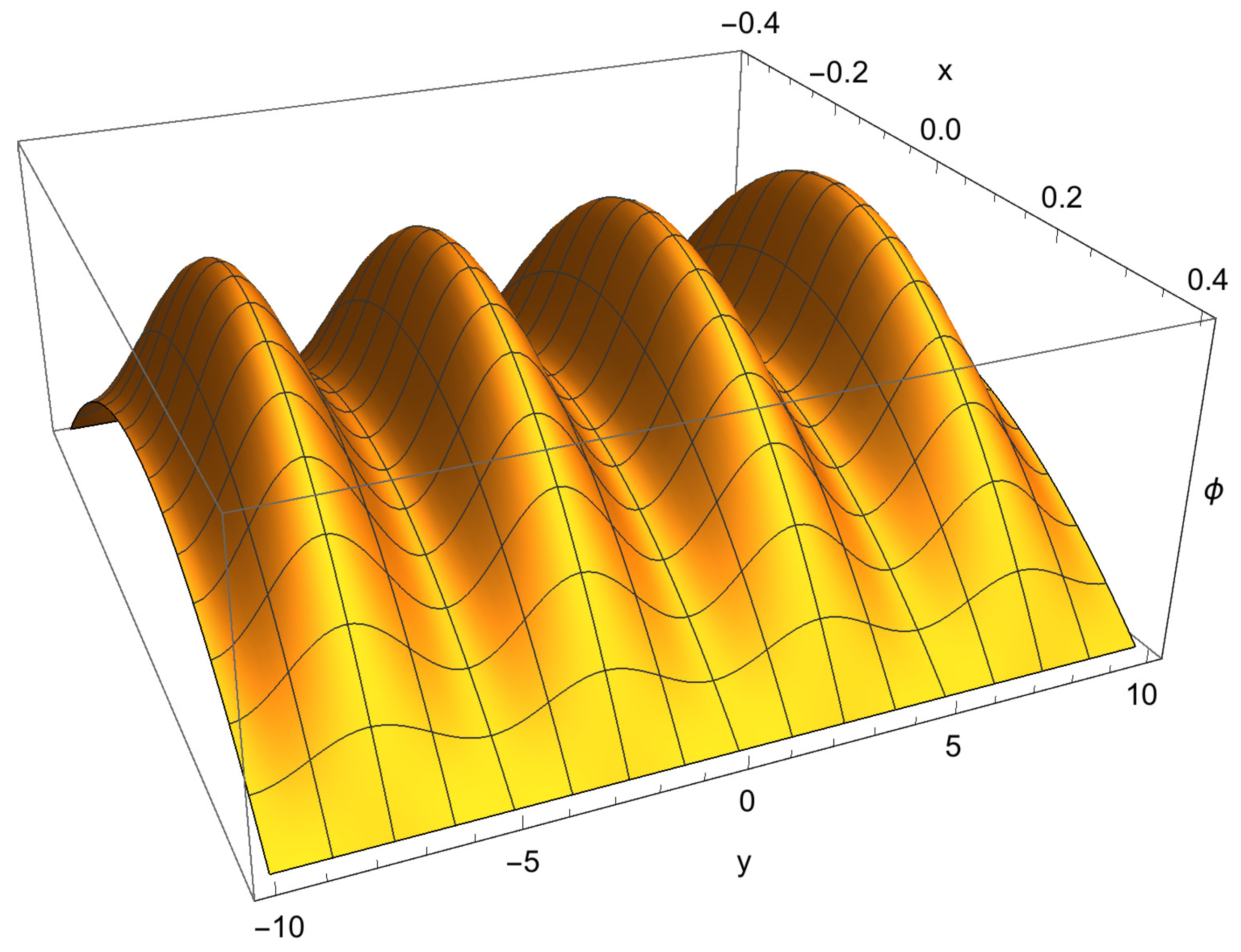
remains non-negative and finite.
Figure 7 shows one such solution with
and
. It is proportional to
, with
. Here
is given by (40) with
,
, and
and
replaced by
and
as given by Equation (
26), respectively.
is also given by (40) with
,
, but with
and
replaced by:
It is also possible to obtain a rectangular unbounded solution by first applying
on the solutions of
. Seeking a finite non-negative value of X(x) again supports the conclusion that no solutions are possible for
values greater than those indicated by the
curve of
Figure 4.
In summary, our consideration of solutions
interior to a rectangular region is compatible with the maximal values of
derived in
Section 3, and shows that exact solutions with varied substructures are possible.
5. Energy Formulation
Let us consider the original equation in (13),
In this section we assume
is an open, bounded subset of
with a smooth boundary (
). Conforming to
Section 3,
so that the fourth-order diffusion term, which dominates at high wave numbers, has negative spectrum, generating a diffusion process that propagates forward in time. With no loss of generality, we set
. Equation (46) is a fourth-order quasi-linear equation in divergence form. Although the fourth-order term
can be written as
, that is, the cascade of two symmetric second-order operators with
, it turns out that
is not symmetric and therefore there is no associated energy functional of which
is the first variation. We introduce the flux potential variable
defined as
where
,
. We also assume
is smooth and strictly positive, implying that
is 1-1 and globally invertible. By substituting
into Equation (46) we obtain:
Here we have defined and . With some abuse of notation—and to keep the notation consistent with the previous sections—in what follows we drop tildas.
We remark that the approach leading to writing Equation (47) is essentially the substitution method largely employed in the theory of porous medium equations [
34]. In soil physics, the variable
u is well known as the matric flux potential [
19,
20]. It is relevant to the physics of the flow since
is the soil–water flux driven by the intrinsic capillary action of the soil matrix, without gravity.
By exploiting the linear structure of the right hand side of (47) the investigation of existence results of the solution becomes more transparent. Let us consider the static problem when
obtained by setting
in Equation (47). Although in this paper we are mainly concerned with time-dependent problems, the static regime is of interest as the solutions of it represent ground-state configurations for the physical system. Eliminating time-dependence in (47) yields:
Equation (48) is obtained as the linear combination of symmetric operators and it does have a variational structure. Indeed, it coincides with the first variation of the functional:
where
. The derivation of (48) from (49) has been performed formally. Under the regularity assumptions on
and if
verifies suitable growth conditions (here unspecified), the derivation of the Euler–Lagrange equation (48) is exact in
. The subspace of
-Sobolev functions
with higher-order energy norm
(where
denotes the Lebesgue space of square-integrable functions) with zero boundary conditions for
u and
, where
is the outward normal to
. Non-homogeneous boundary conditions are incorporated by introducing
, the set containing all the
-functions
u such that
, with
representing the boundary datum.
By exploiting the variational structure of the problem, one may look for solutions to (48) as the critical points of (49) and vice-versa. The nature of the critical points of I is determined by the sign of b as well as the shape of . As an example, when and with , the Lax–Milgram lemma ensures that there exists a unique solution of Equation (48), denoted with , and that is the unique minimizer of in . Furthermore, when , by elliptic bootstrapping we recover that is the classical (indeed in ) solution to Equation (48). From the knowledge of the solution to Equation (48), one is able to recover information on a function which solves the original Equation (46) in the static regime (i.e., ) by simply plugging into Equation (46). In more physically relevant situations represents a competing energy contribution usually in the form of a non-negative multi-well function in the variable u. When is a non-convex non-negative polynomial it may still be possible to ensure the existence (although not the uniqueness) of the solution to the minimum problem for possibly in a subset of and characterize as a solution to Equation (48). Instead, when and with we have genuine competition in the summands of the energy I and in turn I may fail to be positive-definite. Under these circumstances, solutions to Equation (48) correspond to various critical points of I including saddles or more intricate situations. In those cases, existence theorems should be investigated by methods possibly based on min-max principles.
An alternative approach (e.g., [
15,
16]) is to express the phase flux density as being proportional to the negative gradient of a chemical potential energy density that is itself the variational derivative of a total internal energy functional. This comes about because the drift velocity of the mobile particles of Phase 1 quickly reaches a terminal velocity that enables the driving gradient of chemical potential energy to be balanced by a mechanical resistance force that is proportional to velocity and in the opposite direction. The new element that we need here to justify the non-standard Equation (
6) is that the variational derivative is taken with respect to the flux potential
u, rather than the phase variable
. Then we choose:
In this set-up, must be regarded as an externally driven Phase 1 production term that assists relaxation towards the stable fixed points.
6. Conclusions
A nonclassical symmetry reduction has led to some exact positive solutions for multi-dimensional nonlinear reaction–diffusion equations with both fourth-order diffusion and second-order backward diffusion. In all likelihood, these are the only known exact solutions for equations of the Allen–Cahn–Hilliard type that have meaningful boundary conditions. The presented solutions have a zero flux and a zero gradient at one central boundary point, plus a prescribed value, representing a pure phase, as well asa zero gradient at the other boundary. The initial condition has the phase field taking the value at . Even though Phase 1 is stabilised by the reaction term, the boundary conditions force the solution to have the system uniformly approaching Phase 0. An interior cylindrical or spherical inclusion with a mixed phase could not withstand the inward advance of Phase 0 from the outer boundary.
Structured phase domain patterns have been seen in numerical solutions of the Cahn–Hilliard equation (e.g., [
35]). Some exact solutions with pronounced sub-structure have been produced here too. Since the exact solution involves a general solution of the fourth-order linear Helmholtz equation for the flux potential, it is possible that more complex patterns could be incorporated in the future. Any solution of the fourth-order Helmholtz equation can be used in this method, even those that apply in more complicated asymmetric domains.
We remark the approach based on the Helmholtz substitution adds additional structure to the model in terms of a variational principle as the by-product of symmetry and linearity. Although the thorough investigation of the relation between the non-linear model in the unknown variable
and the transformed model in
u is not the scope of the present contribution, in
Section 5 some insight is provided for some special situations. The construction used here became possible because of a nonclassical symmetry that applies when the nonlinear diffusivity and the nonlinear reaction term together obey a single relationship. Then an additional constraint
added to the governing PDE, results in an integrable system. Reduction of variables then results in the linear fourth-order Helmholtz equation. In that sense, the original multidimensional nonlinear scalar PDE is partially integrable because one additional constraint leads to a linear PDE with one fewer independent variables. It remains to be discovered whether nonclassical symmetry classification can unearth other semi-integrable PDEs—possibly defined by different fourth-order non-linear operators—in this way, and more generally, how compatible constraints may be selected.


