A Filtering Method for Grain Flow Signals Using EMD Thresholds Optimized by Artificial Bee Colony Algorithm

Abstract

For the purpose of reducing noise from grain flow signal, this paper proposes a filtering method that is on the basis of empirical mode decomposition (EMD) and artificial bee colony (ABC) algorithm. At first, decomposing noise signal is performed adaptively into intrinsic mode functions (IMFs). Then, ABC algorithm is utilized to determine a proper threshold shrinking IMF coefficients instead of traditional threshold function. Furthermore, a neighborhood search strategy is introduced into ABC algorithm to balance its exploration and exploitation ability. Simulation experiments are conducted on four benchmark signals, and a comparative study for the proposed method and state-of-the-art methods are carried out. The compared results demonstrate that signal to noise ratio (SNR) and root mean square error (RMSE) are obtained by the proposed method. The conduction of which is finished on actual grain flow signal that is with noise for the demonstration of the effect in actual practice.

1. Introduction

In the measuring of grain flow, a crucial parameter in the construction of yield map, impact-type flow sensors are always adopted [1]. These sensors are installed on the clean grain elevator’s top. Normally they are subject to excessive noise, which makes it hard to measure precisely. Buried in noise signals, these grain flow signals from these sensors are not available for subsequent processing. As a result, the effect of subsequent processing is under the direct influence of an effective filtering method. Figure 1 shows the above grain flow signal acquisition and processing principle.

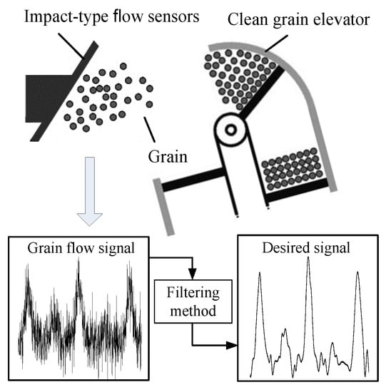
Figure 1. Process of grain flow signal acquisition and processing.

Traditionally, grain flow signal filtering schemes rely on linear methods, for example, moving average [2] or low pass filter [3,4]. The frequent use of these linear methods is due to their easy design and implementation. However, linear filtering methods do not have good effects when sharp edges as well as impulses of short duration are contained in grain flow signal, or when the processing involves transient non-stationary and wide-band components, the spectrum of which is similar to that of the noise. For the purpose of overcoming these obstacles, researchers have proposed nonlinear methods, particularly methods that are on the basis of wavelets and EMD. According to Wang and Hu [5], when EMD was used to finish the removal of noise from grain flow signal, the value of total grain mass’ relative error was under 1.6%. Other filtering noise methods could not achieve a result as good as that. Zhang et al. [6] finished the processing of grain flow signal using the wavelets. In this method, the basis of wavelets is DB9, and the level of decomposition is eight. According to the results, this method performs better in suppressing the noise. Chen et al. [7] also adopted wavelets to finish the removal of noise in grain flow signal. However, their method was not totally the same as that of Zhang. In the latter, the mallat algorithm was introduced for the purpose of decomposing and removing grain flow signal’s noise components.

Inspired by wavelet threshold filtering, EMD threshold filtering was proposed to eliminate the noise components effectively [8]. In comparison with wavelet threshold filtering, EMD threshold filtering has broad application prospects because it is adaptive [9]. In this method, a threshold function was adopted to calculate threshold. While the introduction of threshold improves the filtering ability of EMD, but the threshold function fails to get the optimal threshold to achieve adaptive filtering.

Not long ago, researchers developed swarm intelligence algorithms (SIAs) in threshold filtering for the threshold estimation work. Combination EMD threshold and an improved fruit fly optimization algorithm (IFOA) were proposed to eliminate noise components from machinery sound. The introducing of IFOA was for the purpose of searching each IMF’s global optimal threshold. The proposed method’s effectiveness and superiority were proved through simulation and engineering application [10]. Particle swarm optimization (PSO) was adopted for the purpose of determining the optimal wavelet-filtering threshold. According to the results, the proposed method performed better than state-of-the-art methods. The proposed method could make source signals recovered from a heavy blurred signal, as well as keep source signals’ details from light blurred signals [11]. To choose the best optimization algorithm for EMD threshold, artificial bee colony (ABC), PSO, and cuckoo search (CS) were implemented. As a result, PSO and CS were the best method in terms of attaining maximum SNR as well as MSE [12]. From the above, it can be seen that some results of swarm intelligence algorithms for estimating threshold have been achieved. However, few references about employing ABC to estimate EMD threshold can be found. Therefore, a filtering method, which is on the basis of EMD and ABC, is proposed. This paper’s contribution mainly lies in the methodology illustrating the design as well as application of ABC-optimized EMD threshold.

The specific objectives of this study are to: (1) Develop a new filtering method based on EMD and ABC algorithm, and (2) investigate the results obtained by using different filtering method to remove noise through simulation experiment and practical application.

The rest of this paper is organized as follows: Section 2 introduces related works about EMD threshold filtering method and basic ABC. Section 3 presents our method. Section 4 presents performance comparison between our method and state-of-the-art methods. Section 5 shows the application of proposed method to reduce grain flow signal noise. Section 6 gives some conclusions.

2. Related Works

2.1. EMD Algorithm

The decomposition of a given signal is carried out by EMD through these sifting processes. After the decomposing process, some distinct time scale IMFs are obtained. All the IMFs have to meet two conditions. The first condition is that the number of extreme and these zero crossings’ numbers are either equal to or differ with each other at most by one; the other condition is that at any point, the mean values of local-maxima-defined envelope and the local minima-defined-envelop is zero [13]. When a signal x(t) is given, the following steps are involved in the EMD sifting process:

Step 1: Identifying all extreme of x(t), and constructing its upper envelope h(t) and lowering envelope l(t) through making all local maxima and minima with cubic spline functions connected;

Step 2: Computing the envelopes mean with the formula m(t) = [h(t) + l(t)]/2;

Step 3: Extracting the detail e₁(t) = x(t) − m(t);

Step 4: Regarding e₁(t) as new x(t) and repeating the operation above until e₁(t) meet the IMF conditions, then obtaining the first IMF, label as c₁(t) = e₁(t).

Step 5: Setting the residual x(t) = x(t) − e₁(t) to be a new signal, and jump to Step1, obtain the other IMFs.

According to the sifting result, x(t) is decomposed into c_q(t), q = 1, …, p, and a residual r_p(t) given as follow:

$$x(t)={\displaystyle \sum _{q=1}^{p-1}{c}_q(t)+r_p(t)}$$

(1)

2.2. EMD Filtering Method

Through threshold process the IMFs before reconstructing signals, the input data’s smooth version can be got. When $T=[{\tau }_1,{\tau }_2,\cdots ,{\tau }_q,\cdots ,{\tau }_p]$ denotes a threshold set, and τ_q represents c_q(t)’s threshold, the determination of τ_q can be finished for the removal of Gaussian white noise as shown in the following [14]:

$${\tau }_q=\frac{{\mathrm{MAD}}_q\sqrt{2\log (L)}}{0.6745}$$

(2)

$${\mathrm{MAD}}_q=\mathrm{Median}\left\{\left|c_q(t)-\mathrm{Median}\left\{c_q(t)\right\}\right|\right\}$$

(3)

where ${\mathrm{MAD}}_q$ represents the qth IMF’s absolute median deviation, and L represents the signal length or the sampling number. Gaussian white noise presents a standard normal distribution. For the standard normal distribution, the error probability fall within the range of 25% to 75% that corresponding to −0.6745 and +0.6745, respectively. These IMF samples are shrunk towards zero by the threshold ${\tau }_q$, which is as follows [15]:

$$b_q(t)=\{\begin{array}{cc}{c}_q(t)-{\tau }_q& \mathrm{if}{c}_q(t)\ge {\tau }_q\hfill \\ 0& \mathrm{if}\left|c_q(t)\right|<{\tau }_q\hfill \\ c_q(t)+{\tau }_q& \mathrm{if}{c}_q(t)\le -{\tau }_q\hfill \end{array}$$

(4)

The presenting of the filtered signal y(t) can be made as follows:

$$y(t)={\displaystyle \sum _{q=1}^{p-1}{b}_q(t)}$$

(5)

Above all, Figure 2 shows the threshold-based EMD filtering method’s schematic diagram.

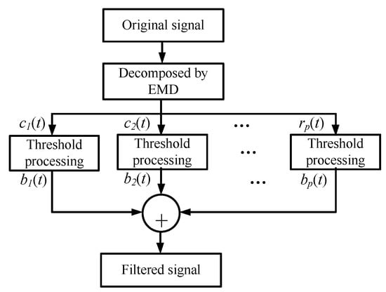
Figure 2. Schematic diagram of EMD filtering method based on thresholds.

2.3. Basic ABC Algorithm

ABC algorithm inspired by honey-bees’ behaviors is used for solving complex optimization problems [16,17,18,19]. This algorithm involves three kinds of bees. They are employed, onlooker and scout bees. Information of the food sources is shared among these different kinds of bees. Employed bees are responsible for finding the food sources and delivering the food sources’ information to onlooker bees in their hive. Onlooker bees are following employed bees to find the food sources according to the information received by them. In food sources exploring process, if there is no improvement in a food source after the conduction of successive trials of a pre-determined number, the employed bee will abandon the food sources, and the employed bee related to the food source will become a scout who searches around randomly. The name of the number of trials to release a food source is “limit”, and in the ABC algorithm, “limit” is a crucial control parameter. The following shows the procedure of ABC algorithm:

Step 1: Generating N food sources randomly:

$$x_{ij}=x_j^{\min }+\mathrm{rand}[0,1](x_j^{\max }-x_j^{\min })$$

(6)

where $x_{ij}$ means that artificial bee is in ith food source’s jth position; $i=1,2,\cdots ,N$; $j=\mathrm{rand}[1,2,\cdots ,n]$; Here, N represents the number of food sources, and n represents the dimension of the search space; $x_j^{\min }$ and $x_j^{\max }$ represent the jth variable’s lower and upper bounds, respectively.

Step 2: When the present food position is X_i = [x_i1, x_i2, …, x_in], the employed bees use the following solution search equation for the purpose of generating a new food source V_i = [x_i1, x_i2, …, v_ij, …, x_in].

$$v_{ij}=x_{ij}+{\theta }_{ij}(x_{ij}-x_{kj})$$

(7)

where $v_{ij}$ means that the position of the new source is found by the ith employed bee, $i=1,2,\cdots ,\mathrm{N}$, $j=\mathrm{rand}[1,2,\cdots ,n]$ and $\begin{array}{cc}k\in \{1,2,\cdots ,N\}& k\ne i\end{array}$. ${\theta }_{ij}$ is a random number that is selected from [−1, 1].

Step 3: all the onlooker bees choose and follow the employed bees according to the food sources’ quality. The calculation of the quality, which is denoted as P_i, is as follows;

$$P_i=\frac{fi{t}_i}{{\displaystyle \sum _{i=1}^{N}fi{t}_i}}$$

(8)

where fit_i represents the ith solution’s fitness.

Step 4: When no improvement of a food sources is observed after trails of the predetermined number “limit”, it will be supposed that the food source will be abandoned, after which the employed bees will become scouts. After this, the production of a new food source will be made randomly in the searching space using (6).

3. The Proposed Method

This paper proposes a filtering method that is on the basis of EMD threshold, which is optimized by the ABC algorithm for the purpose of adaptively eliminating noise components from signal. Figure 3 illustrates the proposed method’s schematic diagram.

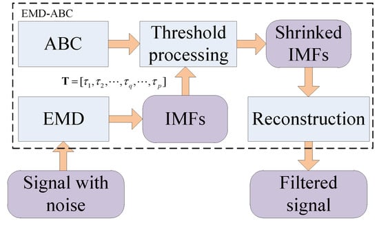
Figure 3. Schematic diagram of EMD-IABC.

It is often hard and time-consuming to determine EMD threshold since their estimation is in accordance with statistic and experiment analysis. In addition, the noise elimination process based on EMD gets important efficiency from an appropriate threshold. In this paper, the determination of thresholds $T=[{\tau }_1,{\tau }_2,\cdots ,{\tau }_q,\cdots ,{\tau }_p]$ is performed automatically by using ABC algorithm.

ABC algorithm has its drawbacks for solving complex problems, including premature convergence and slow convergence speed. A potential reason for these is that the fitness landscape is also very rugged especially for a multimodal problem. However, local optimum may be in close to the global optimum particularly for the complex optimization problem. When a current solution is unfortunately trapped in local optimum, searching its neighborhoods is effective to find better solutions or the global optimum. Based on this viewpoint, a new neighborhood search strategy (NSS) is employed in the basic ABC algorithm, and is expressed as:

$$v_{iq}=\{\begin{array}{c}{a}_1\cdot {\tau }_{best}+a_2({\tau }_{iq}-{\tau }_{kq})\\ {\tau }_{best}+{\theta }_{ij}({\tau }_{iq}-{\tau }_{kq})\\ v_{iq}\end{array}\begin{array}{c}\mathrm{if}fi{t}_i^{\prime }<fi{t}_i,fi{t}_i^{″}\\ \mathrm{if}fi{t}_i<fi{t}_i^{\prime },fi{t}_i^{″}\\ \mathrm{otherwise}\end{array}$$

(9)

where ${\tau }_{best}$ is the best food source in the all food source. The indices a₁ and a₂ are mutually exclusive integers randomly chosen from [0, 1], and a₁ + a₂ = 1, a₁ and a₂ are regenerated in each generation, but they remain unchanged for all dimensions of each generation. Once a new food source is generated, the previous food source must compete with it to the next generation. This means that a food source with better fitness value have the chance to survive. $fi{t}_i{}^{\prime }$ represents the fitness value, which is corresponding to term $a_1\cdot {\tau }_{best}+a_2\cdot ({\tau }_{iq}-{\tau }_{kq})$, $fi{t}_i$ represents fitness value which is corresponding to term ${\tau }_{best}+{\theta }_{iq}({\tau }_{iq}-{\tau }_{kq})$, $fi{t^{″}}_i$ represents fitness value which is corresponding to term $v_{ij}$. Term $a_1\cdot {\tau }_{best}+a_2\cdot ({\tau }_{iq}-{\tau }_{kq})$ can increase searching speed due to a single direction search around the best solution, which could be trapped in local optimum because indices a₂ is from [0, 1]. But term ${\tau }_{best}+{\theta }_{iq}({\tau }_{iq}-{\tau }_{kq})$ is a two- direction search mechanism because indices ${\theta }_{iq}$ is from [−1, 1], which enhances the exploration ability of the algorithm and is helpful to jump out of local optimum. Therefore, term $a_1\cdot {\tau }_{best}+a_2\cdot ({\tau }_{iq}-{\tau }_{kq})$ and term ${\tau }_{best}+{\theta }_{iq}({\tau }_{iq}-{\tau }_{kq})$ are combined for the balance of exploitation and exploration.

RMSE, short for the root mean square error, refers to the degree of the reconstructed signal’s deviation with the ideal signal in mean square. However, few of ideal signals are predictable. As a result, the GCV, which is short for generalized cross validation criterion, is adopted as the fitness for selecting threshold in this paper [20]. The GCV does not require an estimation of the noise variance, and is calculated as follows:

$$fit=\frac{\frac{1}{p}{\displaystyle \sum _{q=1}^p{\left[c_q(t)-b_q(t)\right]}^2}}{{\left(\frac{p_0}{p}\right)}^2}$$

(10)

where p represents the number of IMFs, p₀ represents the number of IMFs that is set to 0 in the shrinking process.

In short, the proposed ABC variant in this paper is called NSSABC, and our proposed filtering method combining EMD and NSSABC is referred to as EMD-NSSABC. The proposed filtering method flow is described in the following.

Step 1: Initiation of parameters. Initializing NSSABC’s colony size, maximum cycle number and limit value.

Step 2: Signal decomposition. EMD is used to decompose the original signal.

Step 3: Threshold optimization. Automatic determination of the thresholds $T=[{\tau }_1,{\tau }_2,\cdots ,{\tau }_q,\cdots ,{\tau }_p]$ is realized by the NSSABC.

Step 3.1: Determining the positions of neighbor food source (T₁, T₂, …, T_N) for these employed bees using Equation (7).

Step 3.2: Calculating fitness value using Equation (10).

Step 3.3: Selecting a source of food for an onlooker bee using Equation (8).

Step 3.4: Determining the positions of neighbor food source for these onlooker bees using Equation (9).

Step 3.5: Finding the abandoned food source and allocating its employed bee as a scout for the search of new food sources using Equation (6).

Step 3.6: Memorizing the position of the best food source.

Step 4: Iteration termination. If the number of the maximum cycle is attained, optimal thresholds $T_{best}=[{\tau }_1,{\tau }_2,\cdots ,{\tau }_q,\cdots ,{\tau }_p]$ are recorded, and then stop, and go to Step 3 if that is not the case.

Step 5: IMFs shrinkage. Each IMF is shrunk by Equation (4) with optimal thresholds $T_{best}=[{\tau }_1,{\tau }_2,\cdots ,{\tau }_q,\cdots ,{\tau }_p]$.

Step 6: Signal reconstruction. All IMFs after shrinkage are superposed then filtered signal would be obtained.

4. Simulation Analyses

4.1. Benchmark Signals

To test the performance of the proposed filtering methods, four benchmark signals: Bumps, Doppler, Heavysine, and Blocks are used to perform numerical simulations. Four benchmark signals with size 4096 are corrupted by Gaussion white noise that make SNR maintaining at 2 dB (dB is a pure counting unit and is to represent the ratio of the two quantities). The benchmark signals and the corresponding noisy versions are showed in Figure 4 and Figure 5, respectively.

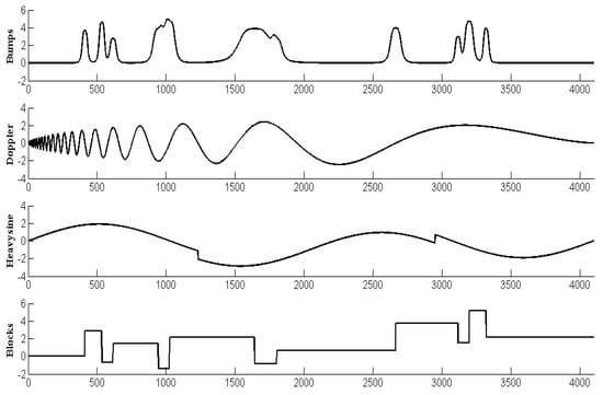
Figure 4. Four benchmark signals.

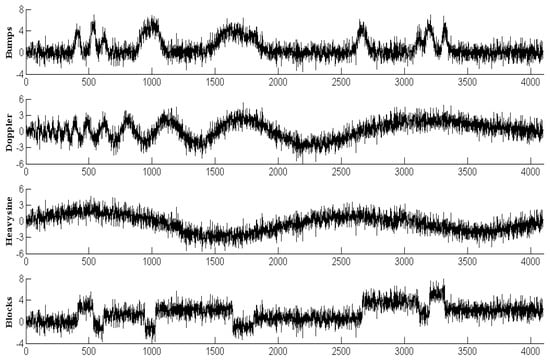
Figure 5. Four Corresponding noisy versions.

4.2. Comparison with Other Filtering Methods

In this subsection, a comparative study between EMD-NSSABC and other four EMD-SIAs is presented. The four SIAs are improved fruit fly optimization algorithm (IFOA) [10], particle swarm optimization with low discrepancy sequence initialized particles and high-order nonlinear dynamic varying inertia weight (LHNPSO) [21], elite-guided genetic algorithm (EGA) [22], and basic ABC. The basic ABC provides a deep insight into the effect of the proposed method. So there are totally five different algorithms in this simulation test, including EMD-IFOA, EMD-LHNPSO, EMD-ABC, and EMD-NSSABC. Parameters setting for five filtering methods are set as follows:

EMD-IFOA: The fruit fly population size was set to 3; fruit fly number in each population was set to 10; fly distance range was set to 1; the variation coefficient was set to 0.2 and the disturbance coefficient was set to 5.

EMD-LHNPSO: The acceleration coefficients c₁ and c₂ were set to 2; the weight coefficients w_min and w_max were set to 0.4 and 0.9, respectively; the population size was equal to 100; the number of non-significant improvements was equal to 5.

EMD-ESLGA: Maximum number of parents was set 12; statistical significance level was equal to 0.05; Population size was equal to 100; elite eligibility threshold was set to 0.9.

EMD-ABC: Population size was equal to 100; the limit was calculated as follows [23]:

$$limit=0.6\times CS\times D$$

(11)

where CS is population size, D is the number of IMFs.

EMD-NSSABC: Parameter settings are same as those of EMD-ABC.

In addition, for all filtering methods, the stopping criterion in EMD was set to 0.25 [13], the iteration number was set to 100, and the initial threshold $T=[0,0\cdots 0]$.

Figure 6 displays the outcome of applying the five EMD-SIAs filtering methods to the four benchmark signals. Globally, the five EMD-SIAs filtering methods do well in reduction of noise and make filtered signals close to the original signals. However, it is difficult to evaluate which method is good or bad from Figure 5, so noise-signal ratio (SNR) and root mean squared error (RMSE) were calculated as the measures of efficiency of noise reduction, which were calculated as follows:

$$\mathrm{SNR}=10{\log }_{10}\frac{{\displaystyle \sum _{m=1}^L{\left[s(m)\right]}^2}}{{\displaystyle \sum _{m=1}^L{\left[y(m)-s(m)\right]}^2}}$$

(12)

$$\mathrm{RMSE}=\sqrt{\frac{1}{L}{\displaystyle \sum _{m=1}^L{\left[s(m)-y(m)\right]}^2}}$$

(13)

where L denotes sampling number, $s(m)$ denotes the original signal, and y(m) is the filtered signal.

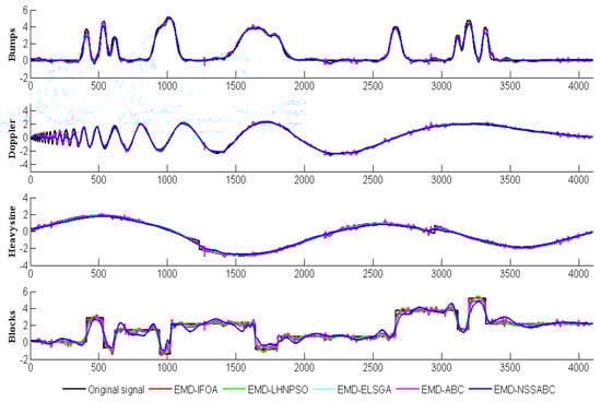
Figure 6. Filtering results with the five-filtering method.

As Table 1 show, the EMD-NSSABC obviously occupied the advantages of SNR and RMSE in comparison with the other four filtering methods. Specifically, compared with the basic ABC, the EMD-NSSABC outperforms it on four benchmark signals: For Bumps, Doppler, Heavysine, and Blocks signals, RMSE reduces by 17.78%, 18.75%, 34.48%, and 22.45% (computing method: $\frac{\left|{\mathrm{RMSE}}_{\mathrm{EMD}-\mathrm{NSSABC}}-{\mathrm{RMSE}}_{\mathrm{EMD}-\mathrm{ABC}}\right|}{{\mathrm{RMSE}}_{\mathrm{EMD}-\mathrm{ABC}}}\times 100\%$), and SNR increases by 17.67%, 15.12%, 7.26% and 10.85% (computing method: $\frac{\left|{\mathrm{SNR}}_{\mathrm{EMD}-\mathrm{NSSABC}}-{\mathrm{SNR}}_{\mathrm{EMD}-\mathrm{ABC}}\right|}{{\mathrm{SNR}}_{\mathrm{EMD}-\mathrm{ABC}}}\times 100\%$). Table 1 results illustrate that the threshold obtained by the NSSABC are superior to that get by the other four SIAs, and imply that with the new neighborhood search strategy, the NSSABC has more exploration ability than the basic ABC.

Table 1. The filtering performance of the five methods.

Method	Bumps		Doppler		Heavysine		Blocks
	SNR	RMSE	SNR	RMSE	SNR	RMSE	SNR	RMSE
EMD-IFOA	10.69	0.43	11.17	0.41	19.25	0.22	11.26	0.43
EMD-LHNPSO	10.27	0.41	11.15	0.45	19.35	0.21	11.42	0.40
EMD-ESLGA	10.38	0.42	11.13	0.43	19.14	0.25	11.36	0.42
EMD-ABC	9.79	0.45	10.12	0.48	18.96	0.29	11.15	0.49
EMD-NSSABC	11.52	0.37	11.65	0.39	20.23	0.19	12.36	0.38

To clearly show the convergence rate, the convergence curves of EMD-IFOA, EMD-LHNPSO, EMD-ESLGA, EMD-ABC and EMD-NSSABC are plotted in Figure 7, which clearly indicates that EMD-NSSABC is better than EMD-IFOA, EMD-LHNPSO, EMD-ESLGA, and EMD-ABC, respectively, regarding to convergence speed on four benchmark signals. This result demonstrates that the new neighborhood search strategy can enhance the exploitation of ABC and accelerate the convergence speed. In summary, through introduction of new neighborhood search strategy, the performance of the basic ABC can be further significantly improved, and then the filtering performance of EMD is enhanced effectively.

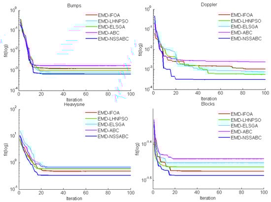
Figure 7. Convergence curves of five methods for four benchmark signals.

For the purpose of researching the filtering performance at different levels of noise, a further comparison was performed for four noise levels, which were 4 dB, 6 dB, 8 dB, and 10 dB, respectively. As Figure 8 shows, for four benchmark signals, the EMD-NSSABC still kept the best filtering effect with increasing noise level among five filtering methods. A group including EMD-IFOA, EMD-LHNPSO, and EMD-ELSGA is secondary compared with EMD-NSSABC in term of SNR, and the three methods’ SNR do not show an obvious difference. The last one is the EMD-ABC due to no improvement in the basic ABC. A similar comparison in term of RSME is presented in Figure 9. As seen in Figure 9, RSME increases gradually with the increasing noise level and obtained a minimum value at the EMD-NSSABC. Through the comparison, we can draw a conclusion that the EMD-NSSABC shows noticeable advantages over other EMD-SIAs methods and is robust to different noise levels.

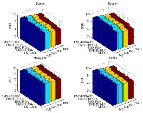
Figure 8. The SNR for the five methods in different noise level.

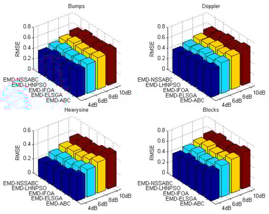
Figure 9. The RMSE for the five methods in different noise level.

5. EMD-NSSABC in Application

A test rig was established for the purpose of testing the EMD-NSSABC’s practical performance for grain flow signal. As shown in Figure 10, Grain flow signals were got from the test rig. There were some experiment conditions. First, the clean grain elevator’s top was installed with a novel grain flow sensor, which using PVDF piezoelectric film as the active to measure the impact force [24,25], the structure of novel sensor used in this paper is shown in Figure 11. Second, measuring of the grain flow was finished through by the weighing sensor with an accuracy of 0.05%. Third, measuring of the sprocket rotational speed was made by the speed sensor. The sprocket rotational speed was changed by using the motor and the frequency converter. Fourth, it is necessary to use signal modulate circuit in order to bring signals to an appropriate range for recording. In addition, NI USB-6216 card as well as computer and LABVIEW software were included in the data acquisition system, and the sampling rate was set to be 1 kHz.

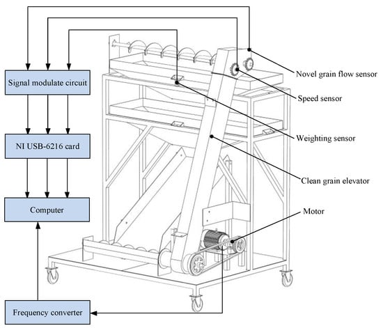
Figure 10. Schematic of test rig for selecting grain flow signal.

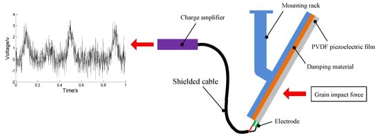
Figure 11. Structure and principle of novel grain flow sensor.

The PVDF piezoelectric film is force-sensitive element of the sensor with size 220 mm × 180 mm × 0.07 mm and piezoelectric constant d₃₃ = 200 pc/N. The damping material plays an important role of buffer effect for PVDF piezoelectric film. The mounting rack make PVDF piezoelectric film fixed at the exit of clean grain elevator. The charge amplifier outputs voltage that is proportional to the grain impact force.

Since there were a lot of noise signals in the grain flow signal, reducing the collected grain flow signal’s noise was of great importance for the improvement of the grain flow’s measurement accuracy. For the purpose of validating the EMD-NSSABC’s effectiveness and superiority, a piece of grain flow signal from the test rig was collected and analyzed. The grain flow signal with noise as well as the filtered grain flow signal are shown in Figure 12. In the Figure 12, the EMD-NSSABC’s effect on the grain flow signal with noise are shown in a clear way. Besides conserving the grain flow signal’s overall trend, the filtered grain flow signal can also restore the weak grain flow signal that is drowned in noise. Table 2 also shows that the EMD-NSSABC perform better than the other four methods in practical application. Altogether, there are five pulses in the grain flow signal, and the 4th pulse in the grain flow with noise is not strong enough to distinguish from noise. However, it is easy to identify it in filtered grain flow signal. Thus, the filtered grain flow signal more suits for further processing.

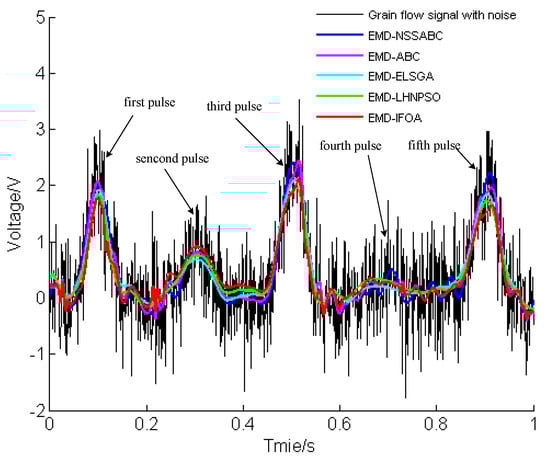
Figure 12. The grain flow signal with noise and the filtered grain flow signal.

Table 2. Application comparison of the five methods.

	SNR	RMSE
EMD-IFOA	9.79	0.52
EMD-LHNPSO	9.28	0.61
EMD-ESLGA	9.48	0.57
EMD-ABC	8.73	0.65
EMD-NSSABC	10.26	0.49

6. Conclusions

This paper proposed an EMD threshold-based filtering method, which is optimized by the ABC for the purpose of reducing noise in grain flow signal. To balance exploration and exploitation ability of ABC and then search optimal thresholds, the neighborhood search strategy is integrated into ABC (NSSABC). To comprehensively investigate the proposed method, four benchmark signals is used in the experiments, and five different EMD-SIAs methods are included in the comparison studies, including the EMD-NSSABC, the EMD-IFOA, the EMD-LHNPSO, the EMD-ELSGA, and the EMD-ABC. The compared results demonstrate the proposed method can offer better performance on four benchmark signals. Even when the noise level increases, the proposed method still performs better than the other four EMD-SIAs methods. Moreover, the proposed method has been verified in a grain flow test rig. It can well eliminate noise and restore grain flow signal, proving its effectiveness and superiority in filtering out noise in a complex environment.

References

- Reinke, R.; Dankowicz, H.; Phelan, J.; Kang, W. A dynamic grain flow model for a mass flow yield sensor on a combine. Precis. Agric. 2011, 12, 732–749. [Google Scholar] [CrossRef]
- Shoji, K.; Matsumoto, I.; Kawamura, T. Impact-by-impact sensing of grain flow on jidatsu combine. Eng. Agric. Environ. Food 2011, 4, 1–6. [Google Scholar] [CrossRef]
- Hamrita, T.K.; Durrence, J.S.; Vellidis, G.; Perry, C.D.; Thomas, D.L.; Kvien, C.K. Noise reduction in a load cell based peanut yield monitor using digital signal processing techniques. In Proceedings of the Thirty-Fifth IAS Annual Meeting and World Conference on Industrial Applications of Electrical Energy, Rome, Italy, 8–12 October 2000; pp. 1008–1015. [Google Scholar]
- Pelletier, G.; Upadhyaya, S.K. Development of a tomato load/yield monitor. Comput. Electron. Agric. 1999, 23, 103–117. [Google Scholar] [CrossRef]
- Wang, H.; Hu, J. Grain flow signal reduction noise using EMD. Int. Agric. Eng. J. 2015, 24, 152–158. [Google Scholar]
- Zhang, X.; Hu, X.; Zhang, A.; Zhang, Y.; Yuan, Y. Method of measuring grain-flow of combine harvester based on weighing. Trans. Chin. Soc. Agric. Eng. 2010, 26, 125–129. [Google Scholar]
- Chen, J.; Wang, K.; Li, Y. Wavelet denoising method for grain flow signal based on Mallat algorithm. Trans. Chin. Soc. Agric. Eng. 2017, 33, 190–197. [Google Scholar]
- Boudraa, A.O.; Cexus, J.C. EMD-based signal filtering. IEEE Trans. Instrum. Meas. 2007, 56, 2196–2202. [Google Scholar] [CrossRef]
- Boudraa, A.O.; Cexus, J.C.; Saidi, Z. EMD-based signal noise reduction. Int. J. Signal Process. 2004, 1, 33–37. [Google Scholar]
- Xu, J.; Wang, Z.; Tan, C.; Si, L.; Liu, X. A novel denoising method for an acoustic-based system through empirical mode decomposition and an improved fruit fly optimization algorithm. Appl. Sci. 2017, 7, 215. [Google Scholar] [CrossRef]
- Liu, C.C.; Sun, T.Y.; Tsai, S.J.; Yu, Y.H.; Hsieh, S.T. Heuristic wavelet shrinkage for denoising. Appl. Soft Comput. 2011, 11, 256–264. [Google Scholar] [CrossRef]
- Jain, S.; Bajaj, V.; Kumar, A. Effective denoising of ECG by optimized adaptive thresholding on noisy modes. IET Sci. Meas. Technol. 2018, 12, 640–644. [Google Scholar] [CrossRef]
- Huang, N.E.; Shen, Z.; Long, S.R.; Wu, M.C.; Shih, H.H.; Zheng, Q.; Yen, N.-C.; Tung, C.C.; Liu, H.H. The empirical mode decomposition and the hilbert spectrum for nonlinear and non-stationary time series analysis. Proc. Math. Phys. Eng. Sci. 1998, 454, 903–995. [Google Scholar] [CrossRef]
- Donoho, D.L.; Johnstone, I.M. Ideal spatial adaptation by wavelet shrinkage. Biometrika 1994, 81, 425–455. [Google Scholar] [CrossRef]
- Donoho, D.L. De-noising by soft-thresholding. IEEE Trans. Inf. Theory 1995, 41, 613–627. [Google Scholar] [CrossRef]
- Karaboga, D.; Basturk, B. On the performance of artificial bee colony (abc) algorithm. Appl. Soft Comput. J. 2008, 8, 687–697. [Google Scholar] [CrossRef]
- Wang, H.; Liang, H.; Gao, L. Using an Improved Artificial Bee Colony Algorithm for Parameter Estimation of a Dynamic Grain Flow Model. Math. Probl. Eng. 2018, 2018, 2132963. [Google Scholar] [CrossRef]
- Karaboga, D.; Aslan, S. Discovery of conserved regions in DNA sequences by Artificial Bee Colony (ABC) algorithm based methods. Nat. Comput. 2018, 1–18. [Google Scholar] [CrossRef]
- Mikaeil, R.; Haghshenas, S.S.; Hoseinie, S.H. Rock penetrability classification using artificial bee colony (abc) algorithm and self-organizing map. Geotech. Geol. Eng. 2017, 7, 1–10. [Google Scholar] [CrossRef]
- Reeves, S.J.; Mersereau, R.M. Blur identification by the method of generalized cross-validation. IEEE Trans. Image Process. 1992, 1, 301–311. [Google Scholar] [CrossRef] [PubMed]
- Yang, C.; Gao, W.; Liu, N.; Song, C. Low-discrepancy sequence initialized particle swarm optimization algorithm with high-order nonlinear time-varying inertia weight. Appl. Soft Comput. 2015, 29, 386–394. [Google Scholar] [CrossRef]
- Contaldi, C.; Vafaee, F.; Nelson, P.C. Bayesian network hybrid learning using an elite-guided genetic algorithm. Artif. Intell. Rev. 2018, 1–28. [Google Scholar] [CrossRef]
- Gao, W.; Liu, S.; Huang, L. A global best artificial bee colony algorithm for global optimization. J. Comput. Appl. Math. 2012, 236, 2741–2753. [Google Scholar] [CrossRef]
- Wang, H.; Hu, J.; Gao, L.; Jia, Y. Development and optimization of a novel grain flow sensor based on PVDF piezoelectric film. Int. J. Agric. Biol. Eng. 2016, 9, 141–150. [Google Scholar]
- Wang, H.; Bai, X.; Liang, H. Proportional distribution method for estimating actual grain flow under combine harvester dynamics. Int. J. Agric. Biol. Eng. 2017, 10, 158–164. [Google Scholar]
© 2018 by the authors. Licensee MDPI, Basel, Switzerland. This article is an open access article distributed under the terms and conditions of the Creative Commons Attribution (CC BY) license (http://creativecommons.org/licenses/by/4.0/).