Inconsistent Data Cleaning Based on the Maximum Dependency Set and Attribute Correlation

Abstract

In banks, governments, and Internet companies, inconsistent data problems may often arise when various information systems are collecting, processing, and updating data due to human or equipment reasons. The emergence of inconsistent data makes it impossible to obtain correct information from the data and reduces its availability. Such problems may be fatal in data-intensive enterprises, which causes huge economic losses. Moreover, it is very difficult to clean inconsistent data in databases, especially for data containing conditional functional dependencies with built-in predicates (CFDPs), because it tends to contain more candidate repair values. For the inconsistent data containing CFD^Ps to detect incomplete and repair difficult problems in databases, we propose a dependency lifting algorithm (DLA) based on the maximum dependency set (MDS) and a reparation algorithm (C-Repair) based on integrating the minimum cost and attribute correlation, respectively. In detection, we find recessive dependencies from the original dependency set to obtain the MDS and improve the original algorithm by dynamic domain adjustment, which extends the applicability to continuous attributes and improves the detection accuracy. In reparation, we first set up a priority queue (PQ) for elements to be repaired based on the minimum cost idea to select a candidate element; then, we treat the corresponding conflict-free instance ($I_{nv}$) as the training set to learn the correlation among attributes and compute the weighted distance (WDis) between the tuple of the candidate element and other tuples in $I_{nv}$ according to the correlation; and, lastly, we perform reparation based on the WDis and re-compute the PQ after each reparation round to improve the efficiency, and use a label, flag, to mark the repaired elements to ensure the convergence at the same time. By setting up a contrast experiment, we compare the DLA with the CFD^Ps based algorithm, and the C-Repair with a cost-based, interpolation-based algorithm on a simulated instance and a real instance. From the experimental results, the DLA and C-Repair algorithms have better detection and repair ability at a higher time cost.

1. Introduction

With the development of social informatization, data storage, data analysis, and aid decision-making, relying on various information systems, have occupied a very important position in information society. In the era of the Internet, the data scale has expanded unceasingly due to increasing data requirements and constant shortening of data acquisition and the updating cycle. How to solve data quality problems accompanying big data is an urgent problem for government departments, enterprises, and institutions.

In the field of data quality, data consistency refers to the degree to which a given data set satisfies constraints or the consistency to which the same thing is expressed in the case of multi-source data fusion [1] (pp. 7–18). In this paper, inconsistent data means that a data set does not satisfy the given constraints (such as functional dependencies (FDs) [2] (pp. 426–431), conditional functional dependencies (CFDs) [3] (pp. 537–540), and CFDs with built-in predicates (CFD^Ps) [4] (pp. 3274–3288)). Inconsistent data cannot correctly express the true state of data elements, destroys the relationship between objective things, and greatly reduces the value of data [5] (pp. 1727–1738). For inconsistent data problems in databases, most of the current detection and reparation methods are based on functional dependencies or conditional functional dependencies, which do reparation through the idea of manual intervention, deletion inconsistent tuples, and minimum repair cost.

Currently, the detection and reparation of inconsistent data mainly face two challenges [6] (pp. 41–74): (1) With the gradual expansion of data scale and data constraints, the difficulty of detecting and repairing inconsistent data is multiplied. In this case, there are higher requirements on the convergence and complexity of algorithms. (2) The inconsistent data reparation algorithms are designed to find an optimal result that satisfies the dependencies and conforms to existing rules in data sets as much as possible. However, the candidate repair values of data elements explode with the data scale increasing, which bring great difficulties in the detecting and repairing process.

1.1. Inconsistent Data Cleaning Status

Relevant research [7] (pp. 143–154) has proved that the repair process of inconsistent data is an NP-Complete problem in the case of specified dependencies in data sets, and there are no optimal repair results at a minimum time cost. The existing research results mainly focus on a series of optimization algorithms for databases in various specific fields (such as spatial databases [8] (pp. 280–304) and XML [9] (pp. 1–19)). The general ideas can be divided into the following categories.

Paper [10] (pp. 232–236) proposed an inconsistent data detection and reparation algorithm based on primary key constraints in relational databases, which is a very simple method. The author first defines the primary key and related FDs in the database. The inconsistent data is detected through the uniqueness of the primary key and the given FDs, and then does reparation by deleting tuples with inconsistent data. The advantages of this algorithm are that it is simple and efficient, and it can ensure the rest tuples do not contain any inconsistent elements. However, by deleting tuples to ensure consistency, the data set may lose some critical information, which makes the application field greatly limited.

Another idea to detect and repair inconsistent data is based on CFDs and minimum cost principles. When it comes to repair costs, it is similar to the sorting idea and there are also two totally different ways. Paper [11] considers the smallest difference between original data and repaired data, and chooses their distance (including Euclidean-distance of numbers and Edit-distance of characters) as the repair cost to find a target value with a minimum distance and conflict resolution at the same time. However, the minimum distance is not necessarily the best candidate values. The results obtained only by considering the distance between candidate repair values and original values may not be satisfactory. Paper [12] (pp. 1685–1699) also proposes a method to compute the repair cost; it chooses a value for repair based on the change amount of conflict elements before and after updating all candidate values. All candidate values need to be traversed once before each repair process, which results in high computational complexity in data sets with many candidate values; in this case, the algorithm cannot be applied to large-scale data.

In general, there are several problems in detecting and repairing inconsistent data at present: (1) The detection and reparation algorithms mainly focus on FDs or CFDs, paying less attention to CFD^Ps, while it is much more difficult to detect and repair data violating with CFD^Ps; (2) in the repair process, more consider only RHS (right hand side) of dependencies [13] (pp. 2664–2669), which is obviously unreasonable. The location of error in data sets is often random, so only repairing RHS is more limited; and (3) when selecting a candidate repair value, there is less consideration to the correlation existing in attributes, which means the repaired results may satisfy the given dependencies well, but their authenticity needs further discussion.

We hold the opinion in this paper that it is more credible to repair inconsistent data elements by the existing values in data sets under unsupervised circumstances [14] (pp. 547–554). The main idea is: For given data sets and CFD^Ps, the maximum dependency set (MDS) is obtained to detect and locate the inconsistent elements by finding recessive dependencies contained in CFD^Ps. The dynamic domain adjustment is proposed to improve the original algorithm’s shortcomings to the continuous attributes [15] (pp. 1–18). Then, the priority queue (PQ) of candidate repair values is established based on the located inconsistent elements, selecting the data to be repaired according to the minimum cost idea and computing the correlation among attributes through symmetric uncertainty (SU) in the information theory. At last, the improved KNN algorithm is used to repair the inconsistent data. This algorithm integrates the minimum cost idea and correlation among attributes, and it can be applied to inconsistent data that violates CFD^Ps.

1.2. Purpose and Structure of This Paper

The purpose of this paper is to propose a detection and reparation algorithm for data that violates the CFD^Ps in data sets. The main contributions and innovations are:

(1)

We propose a heuristic algorithm for inconsistent data detection and reparation, which can repair inconsistent data violating the CFD^Ps in data sets under unsupervised circumstances;

(2)

For inconsistent data detection, the maximum dependency set is used to detect them. By finding recessive dependencies from original dependency sets, we improve the detection accuracy and apply the algorithm to continuous attributes; and

(3)

For inconsistent data reparation, we use unsupervised machine learning to learn the correlation among attributes in data sets, and integrate the minimum cost idea and information theory to repair, which makes the repair results most relevant to the initial values with minimum repair times.

The rest of the paper is structured as follows:

In Section 2, after formally describing the inconsistency in databases, we propose an inconsistent data cleaning framework and give an example for readers to understand and reproduce. Then, we design the detection and reparation algorithms and analyze the convergence and complexity of them. In Section 3, to verify the effectiveness of our algorithms, we compare them with other algorithms through different data scales and inconsistent proportions, and then analyze the experimental results. In Section 4, we analyze the advantages and disadvantages of two algorithms in detail, explain the reason why our algorithms perform better, and put forward the subsequent improvement direction. At last, in Section 5, we summarize the contributions of this paper.

2. Materials and Methods

In this Section, we first formally describe the inconsistency in databases, then we propose an inconsistent data cleaning framework and design the detection and reparation algorithms according to it. In detection, we use the MDS to improve the detection accuracy and extend the algorithm to continuous attributes. In reparation, we first set up the PQ based on the minimum cost idea, then we learn the correlation among attributes in the corresponding conflict-free data instance using an unsupervised machine learning method. Finally, we do reparation according to the learned correlation. Moreover, the algorithm does not require manual intervention in the repair process and can be applied to special cases violating CFD^Ps.

2.1. Problem Description

Data consistency means the degree to which elements in a data instance, I, satisfy a dependency set, D. Different from the “equality constraints” of CFDs [16] (pp. 864–868), the CFD^Ps are special forms of dependencies containing predicates [4] (pp. 3274–3288). Intuitively, CFD^Ps are actually extending the “equality constraints” of CFDs to “predicate constraints”. For any tuple, $t_i$, $t_i\in R$, the form of a CFD^P is like “$t_i\left[X\right]>a\to t_i\left[Y\right]>\mathrm{b}$”, and this dependency type is also common in data sets. Compared with “equality constraints” of CFDs, “predicate constraints” are more difficult to detect and repair because they often contain more candidate values.

In semantics, if the $X$ and $Y$ attributes of a tuple, $t_i$ in I ($t_i \in I$) violates the given dependencies, $cf{d}^P$, which means the $X$ attribute of $t_i$ satisfies the LHS (left hand side) of $cf{d}^p$, but the $Y$ attribute violates the RHS, expressed as $t_i\left[X\right]\ne cf{d}^P$ and $t_i\left[Y\right]\ne cf{d}^P$. When describing the inconsistent data elements of $X$ attribute, we still express it as $t_i\left[X\right]\ne cf{d}^P$, because the location of error data is often random.

For the inconsistent data elements detected and located, the following quadruple is used to describe them in this paper:

$$Vcf{d}^p:(t_i,t_i[A_m],t_i[A_n],cf{d}_k^p)$$

(1)

where $t_i$ is the unique identification of a tuple in data instances; $t_i\left[A_m\right]$ and $t_i\left[A_n\right]$ represents the $m_{th}$ and $n_{th}$ attributes of $t_i$, which violate the given dependencies respectively; and $cf{d}_k^P$ means the $k_{th}$ dependency in the dependency set. The location problem of inconsistent data can be solved through Expression (1), which can also facilitate subsequent reparation work.

The following relation schema is given to describe the inconsistent problem in a data set:

staff (id, name, age, excellent_staff, work_seniority, work_place, marry_status, monthly_salary, department)

The meanings, value types, and abbreviations of each attribute in the relation schema are shown in

Table 1. Staff attributes description.

Attributes	Meanings	Value Types	Abbreviations
id	staff number	numeric	ID
name	staff name	text	NM
age	staff age	numeric	AGE
excellent_staff	excellent staff status	boolean	ES
work_seniority	years of work	numeric	WS
work_place	branch office	text	WP
marry_status	marry status	boolean	MSs
monthly_salary	monthly salary	numeric	MSy
department	work department	text	DM

.

For description convenience, subsequent attributes’ descriptions are all represented by the abbreviations in this paper, for example, the ES and MSs respectively indicate excellent staff status and marry status, and the values are T and F.

Selecting part data tuples in the data set, a data instance in the staff relation schema is shown in

Table 2. Staff data instance.

ID	NM	AGE	ES	WS	WP	MSs	MSy	DM
1	Kitty	25	T	4	branch#1	T	3825	security
2	Ming	20	F	2	branch#7	F	4718	manager
3	Wong	18	T	0.5	branch#5	F	3264	personnel
4	Lity	36	F	3.5	branch#1	F	7560	manager
5	John	41	T	5	branch#3	T	5300	communication
6	Li Lei	25	F	4	branch#4	T	3750	sale
7	Lucy	36	T	3	branch#2	F	4103	market
8	Xie Feng	26	F	2	branch#3	T	3520	sale
9	Jack	19	F	1.5	branch#2	F	5030	culture
10	Kai	41	T	5	branch#1	T	7263	manager

.

The following possible dependencies are given to describe the inconsistent data problem in Table 2:

$$cf{d}_1^p：ES=T\to WS\ge 3$$

$$cf{d}_2^p：DM=manager\to MSy\ge 6300$$

$$cf{d}_3^p：WS\ge 1\to AGE\ge 19$$

where $cf{d}_1^P$ indicates the seniority of an excellent staff should be at least three years; $cf{d}_2^P$ means the basic salary of a manager is 6300 RMB; and $cf{d}_3^P$ shows the age of employees whose seniority exceeds one year should be no less than 19 years old. These three dependencies are partial dependencies that may exist in the data instance according to the staff characteristics in a company, and are used to constrain the data in Table 2.

Based on the given $cf{d}^P$, inconsistent data elements existing in Table 2 can be located and expressed by the quadruple in Expression (1). For example, the MSy and DM values of tuple 2 violate the $cf{d}_2^P$, and the ES and WS values of tuple 3 violate the $cf{d}_1^P$, which can be expressed as ($t_2,MSy,DM,cf{d}_2^P$) and ($t_3,ES,WS,cf{d}_1^P$), respectively. In fact, this method, which detects inconsistent data directly through the given $cf{d}^P$, is flawed. We will explain these faults in Section 2.2.1 and use the maximum dependency set to do detection.

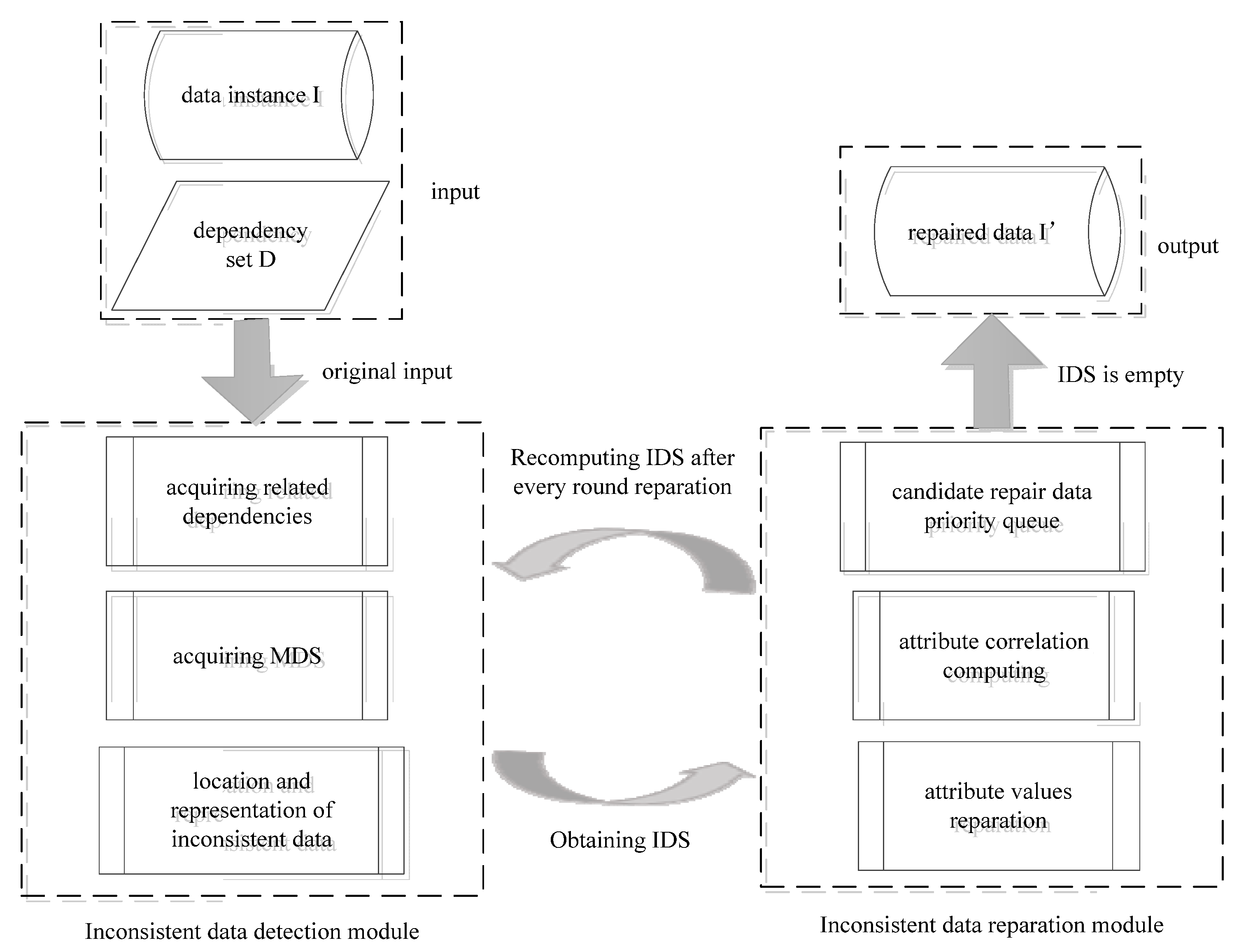
2.2. Inconsistent Data Cleaning Framework

In this section, we propose a framework for inconsistent data detection and reparation. The framework takes a data instance, I, and a dependency set, D, as input, and repaired results, I’ as output, which can detect and repair the inconsistent data in I. It can be divided into two sub-modules: Detection and reparation, as shown in Figure 1. In the framework, the detection module is the foundation of the repair module, taking the detected inconsistent data-elements set (IDS) as input to participate in the repair process, and recalculating the IDS after every reparation round, the repair results will be obtained until the IDS is empty.

In the detection module, referring to the method of obtaining the MDS proposed in [15] (pp. 1–18), we propose the dynamic domain adjustment to improve the original algorithm by setting pointers of a numerical change direction, and extend the algorithm to continuous attributes. As a result, the ability to detect inconsistent data is improved. In the reparation module, we first delete tuples with inconsistent elements to get a conflict-free data instance, $I_{nv}$, as the training set based on the located inconsistent data; at this point, there is no inconsistent data in $I_{nv}$. Then, we consider the correlation among attributes in $I_{nv}$, which is computed by the symmetric uncertainty method in information theory, and select a candidate repair data element according to the established PQ. At last, the improved KNN algorithm is used to do reparation.

2.2.1. Inconsistent Data Detection Module

The inconsistent data detection module detects inconsistent elements in a data instance by obtaining the MDS of a given $cf{d}^P$, and uses the quadruple in Expression (1) to represent and locate. In Section 2.1, we mentioned that the algorithm, which detects inconsistent data directly through the given $cf{d}^P$, is flawed. Then, we will describe these kinds of faults in detail.

Taking the staff data instance in Table 2 and the three $cf{d}^P$ as an example, the inconsistent data elements in staff can be represented as ($t_2,MSy,DM,cf{d}_2^P$) and ($t_3,ES,WS,cf{d}_1^P$) through the three dependencies, $cf{d}_1^P$, $cf{d}_2^P$, and $cf{d}_3^P$. In fact, by analyzing the $cf{d}_1^P$ and $cf{d}_3^P$, it is easy to get a new $cf{d}^P$, called recessive CFD^Ps (RCFD^Ps):

$$rcf{d}_1^p：ES=T\to AGE\ge 19$$

The $rcf{d}_1^P$ is a new dependency obtained by the $cf{d}_1^P$ and $cf{d}_3^P$, which do not exist in the original dependency set. According to the $rcf{d}_1^P$, we can find the AGE and ES attributes in tuple 3 are inconsistent too, expressed as ($t_3,AGE,ES,rcf{d}_1^P$), and this inconsistent data element cannot be detected by the original dependency set. At this point, the $cf{d}_1^P$, $cf{d}_2^P$, $cf{d}_3^P$, and $rcf{d}_1^P$ constitute the MDS of the original dependency set. In this paper, we propose a dependency lifting algorithm (DLA) based on the MDS, which discovers the $rcf{d}^P$ contained in $cf{d}^P$ to obtain the MDS, and do detection by the acquired MDS. Generally, it can be divided into three sub-stages: Acquiring related dependencies, acquiring the MDS and location, and representation of the inconsistent data.

Acquiring Related Dependencies

The process of obtaining the $rcf{d}_1^P$ from the $cf{d}_1^P$, $cf{d}_2^P$, and $cf{d}_3^P$ in Table 2 is used as an example. The DLA first select one attribute in the attribute set ($\mathrm{Attr}\left(\mathrm{R}\right)$) as the start attribute (start_attr), and then computes the $rcf{d}^P$ from all $cf{d}^P$ related to the start_attr. The algorithm ends when all attributes in the data instance, I, are traversed once.

Paper [15] (pp. 1–18) proposed a method to find the $rcf{d}^P$ from the $cf{d}^P$, which defined explicit constraint dependencies through domain knowledge, and got the closed set by mathematical ways [17] (pp. 69–71). This algorithm does set operations by enumerating attribute values, which performs well in discrete data whose attribute values are finite. However, there are two defects in practical application processes: (1) Because the algorithm needs to enumerate all attribute values that do not satisfy the dependencies, it takes a lot of time and space resources to compute in data instances with a large number of dependencies, causing a waste of memory; and (2) since the variance step of continuous attribute values cannot be measured, the algorithm is not suitable for data instances with continuous attributes. We propose a method instead of the enumeration process, and extend the original algorithm to continuous attributes by setting forward pointers (L) and backward pointers (U).

Selecting the ES attribute as the start_attr, the dependencies containing the start_attr are $cf{d}_1^P$ and $cf{d}_3^P$:

$$cf{d}_1^p：ES=T\to WS\ge 3$$

$$cf{d}_3^p：WS\ge 1\to AGE\ge 19$$

Noting the $vio\left(cf{d}_i^P\right)$ is a value space that does not satisfy the $cf{d}_i^P$, the value spaces that do not satisfy the $cf{d}_1^P$ and $cf{d}_3^P$ are shown as follows:

$$vio(cf{d}_1^p)=\{ES:T\}\times \{WS:3,L\}\times \{AGE:all\}$$

$$vio(cf{d}_3^p)=\{WS:1,U\}\times \{AGE:19,L\}\times \{ES:all\}$$

where L and U indicate the value changes to the left and right, respectively; for example, the {$WS:3,L$} means the WS attribute values should be less than three years.

Acquiring the MDS

Acquiring the MDS from a given $cf{d}^P$ is the core of the DLA. For data tuples with N attributes, $T\left(T_1,T_2,T_3,\dots ,T_N\right)$, and an initial dependency set, D, the mathematical forms of obtaining the $rcf{d}^P$ after selecting a start attribute, $T_i$, are shown as follows:

$$RCF{D}^p(i,D)={\displaystyle {\prod }_{j=1}^{i-1}{\cap }_{d\in D}{A}_j^d\times {\cup }_{d\in D}{A}_i^d\times {\displaystyle {\prod }_{j=i+1}^N{\cap }_{d\in D}{A}_j^d}}$$

(2)

In Expression (2), $A_j$ is the values space of the $j_{th}$ attribute, and $A_j^d$ is the values space of the $j_{th}$ attribute, which does not satisfy the dependency, d.

Selecting the WS attribute as the start_attr, and the $vio\left(cf{d}_1^P\right)$ and $vio\left(cf{d}_3^P\right)$ as input, the computing process of obtaining the $rcf{d}_1^P$ is as follows:

$$\begin{array}{l}rcf{d}_1^p(WS,\{vio(cf{d}_1^p),vio(cf{d}_3^p)\})\\ =\{ES:T\}\cap \{ES:all\}\times \{WS:3,L\}\cup \{WS:1,U\}\times \{AGE:all\}\cap \{AGE:19,L\}\\ =\{ES:T\}\times \{WS:all\}\times \{AGE:19,L\}\end{array}$$

where “${\displaystyle \cup }$” and “${\displaystyle \cap }$” operations of the ES, WS, and AGE attributes involves the merging process of different pointers, which are similar to the combination of intervals on a number axis. The WS attribute is shown as an example in Figure 2.

In Figure 2, the {$WS:3,L$} and {$WS:1,U$} are shown in different colors, and the new domain of the WS attribute can be obtained after doing “${\displaystyle \cup }$” operations for two different color areas, that is {$WS:3,L$}${\displaystyle \cup }${$WS:1,U$} = {$WS:\mathrm{all}$}.

In this way, a new dependency, $rcf{d}_1^P$, is obtained:

$$rcf{d}_1^p：ES=T\to AGE\ge 19$$

The MDS will be obtained after all attributes in $\mathrm{Attr}\left(\mathrm{R}\right)$ are traversed once. Then, we judge the data elements in the data instance through the MDS and finally get the inconsistent data.

Location and Representation of Inconsistent Data

For the inconsistent data detected by the MDS, we use the quadruple in Expression (1) to express and locate them. The inconsistent data-elements set (IDS) of staff instance in Table 2 can be expressed as follows:

$$IDS:\{(t_2,MSy,DM,cf{d}_2^p),(t_3,ES,WS,cf{d}_1^p),(t_3,AGE,ES,rcf{d}_1^p)\}$$

(3)

2.2.2. Inconsistent Data Reparation Module

The inconsistent data reparation module takes the repair times of data instances as the repair cost, and first computes the counts of violating dependencies for every inconsistent data element to get the priority queue (PQ). Then, putting the corresponding data instance with no inconsistent data, $I_{nv}$, as the training set, we learn the correlation among attributes in $I_{nv}$ by the symmetric uncertainty method in information theory. At last, we select the candidate repair data element from PQ and do reparation based on the improved KNN algorithm. The whole module takes a data instance, I, and the MDS and the IDS as input, and can also be divided into three sub-stages: Candidate repair data priority queue, attribute correlation computing, and attribute values reparation.

Candidate Repair Data Priority Queue

We choose repair times of the data instance as the repair cost in this paper, establish the PQ based on the IDS, and select the first element from PQ to repair. Taking the $VioCount\left(t_i,A\right)$ as the violation counts of attribute, A, in tuple, $t_i$, for n dependencies in MDS, the way to get $VioCount\left(t_i,A\right)$ can be expressed as follows:

$$VioCount(t_i,A)={\displaystyle \sum _{j=1}^n(A\in cf{d}_j{}^p)}{t}_i,A\in IDS$$

(4)

where $A\in cf{d}_j^P$ means the attribute, A, of the tuple, $t_i$, is contained in a dependency, $cf{d}_j^P$; and $t_i, A\in IDS$ means the attributes of tuples are all selected from the IDS to ensure the selected data elements are all inconsistent.

Taking the MDS and IDS in Section 2.2.1, and the staff instance in Table 2 as an example too, all $VioCount\left(t_i,A\right)$ in IDS are $VioCount\left(t_3,ES\right)$ = 2, $VioCount\left(t_2,MSy\right)= VioCount\left(t_2,DM\right)=VioCount\left(t_3,WS\right)=VioCount\left(t_3,AGE\right)=1$. Then, we establish the PQ according to the $VioCount\left(t_i,A\right)$ and select the first element in PQ to be repaired:

$$PQ:\{(t_3,ES),(t_2,MSy),(t_2,DM),(t_3,WS),(t_3,AGE)\}$$

(5)

Attribute Correlation Computing

When computing the attribute correlation, we need to first delete inconsistent tuples in I to get the corresponding conflict-free data instance, $I_{nv}$, and learn the correlation from the training set, $I_{nv}$. For example, the $I_{nv}$ of the staff instance in Table 2 does not contain tuples, $t_2$ and $t_3$.

In real data sets, there may be a certain correlation among attributes, so it is more advantageous to repair data sets considering the correlation under the unsupervised environment. Generally speaking, in information theory, the way to compute a correlation is the information gain (IG) [18] (pp. 1–8) or the symmetrical uncertainty (SU) [19] (pp. 429–438), however, the disadvantage of the IG is that it tends to select attributes with multiple different values and should be standardized to ensure comparability. In this case, the SU method is chosen to compute in $I_{nv}$.

In information theory, the uncertainty of a variable, X, can be measured by information entropy, $H\left(X\right)$, which increases with the uncertainty of the variable. The mathematical definition is as follows:

$$H(X)=-{\displaystyle \sum _{x\in X}p(x){\log }_{2}p(x)}$$

(6)

where $p\left(x\right)$ means the probability that a variable, X, takes the value of x. The conditional entropy, $H(X|Y)$, represents the uncertainty of a variable, X, when the Y is determined.

$$H(X|Y)=-{\displaystyle \sum _{y\in Y}p(y){\displaystyle \sum _{x\in X}p(x|y){\log }_{2}p(x|y)}}$$

(7)

In Expression (7), $p(x|y)$ means the probability that the variable, X, takes the value of x when the variable Y is y. In this case, the IG can be expressed as:

$$IG(X,Y)=H(X)-H(X|Y)$$

(8)

To eliminate the influence of variable units and variable values, the SU method is used to normalize the IG:

$$SU(X,Y)=2\times \left[\frac{IG(X,Y)}{H(X)+H(Y)}\right]$$

(9)

Taking the staff instance in Table 2 as an example, the $I_{nv}$ can be obtained as $I_{nv}=\left\{t_1,t_4, t_5, t_6, t_7, t_8, t_9, t_{10}\right\}$. In view of the ES attribute, its domain contains two elements {T, F} with the probabilities both 1/2; that is, p(T) = p(F) = 4/8 = 1/2, so the information entropy of the ES is H(ES) = 1 using the method in Expression (6). Similarly, the domain of the AGE attribute is {25, 36, 41, 26, 19} with the probabilities, p(25) = p(36) = p(41) = 2/8 = 1/4, p(26) = p(19) = 1/8, so the information entropy is H(AGE) = 2.25. When the AGE attribute value is 25, the ES attribute values are T and F, and the probabilities are both 1/2; that is p(ES = T|AGE = 25) = p(ES = F|AGE = 25) = 1/2. In a similar way, the conditional probability of the ES attribute when the AGE attribute takes other values can be computed. Then, the conditional entropy, H(ES|AGE), can be obtained based on Expression (7), H(ES|AGE) = 0.5. According to Expression (8), the IG can be computed too, IG(ES, AGE) = H(ES)-H(ES|AGE) = 0.5. At last, the correlation between the ES and AGE attributes through Expression (9) is:

$$SU(ES,AGE)=2\times (\frac{0.5}{1+2.25})=0.31$$

Similarly, the correlation between the ES and other attributes, ID, NM, WS, WP, MSs, MSy, and DM, is 0, 0, 0.43, 0.11, 0.05, 0, and 0.43, respectively. It must be noted that because there are only eight tuples in $I_{nv}$, the correlation among attributes learned from the $I_{nv}$ can only represent the correlation in Table 2, and may not be representative of the whole industry.

Attribute Values Reparation

In the stage of attribute values reparation, we choose the first element in PQ as the candidate repair data element, and compute the distance between tuples according to the improved KNN algorithm and the correlation. The improved KNN algorithm takes the SU among attributes as weight to get the weighted distance (WDis) of tuples, which can be expressed as follows:

$$WDis(t_i,t_j)=\sqrt{{\displaystyle \sum SU(X,Y)\times RDis(t_i[Y],t_j[Y])}}X\in PQ,Y\in \mathrm{Others}$$

(10)

where SU(X,Y) means the correlation between the X and Y attributes, X is the attribute of the candidate repair data element, and Y is another attribute in the data instance. The $RDis\left(t_i\left[Y\right], t_j\left[Y\right]\right)$ means the relative distance between tuples, $t_i$ and $t_j$, on the attributem Y. Due to different types of attributes (numeric, text, and boolean), it is not comparable directly through the Euclidean distance or the edit distance. Therefore, we choose the relative distance (RDis) to measure the distance among attributes in tuples in this paper, which makes the comparability between different types of attributes. For numerical attributes, the ratio of their Euclidean distance to the larger value is computed as the RDis, and for others, the ratio of their edit distance to the longer string is computed as the RDis.

$$RDis(t_i[Y],t_j[Y])=\{\begin{array}{c}\frac{EucD(t_i[Y],t_j[Y])}{max(t_i[Y],t_j[Y])}Y\in numeric\\ \frac{EditD(t_i[Y],t_j[Y])}{maxlen(t_i[Y],t_j[Y])}Y\in others\end{array}$$

(11)

where EucD and EditD represent the Euclidean distance and the edit distance, respectively. Thanks to the relative distance, the distance of attributes in different tuples can be well mapped to the interval [0,1], which makes them comparable.

Taking tuples, $t_3$ and $t_1$, in Table 2 as an example, the candidate repair data element selected from PQ is ($t_3, ES$), and the correlation between the ES and other attributes{ID, NM, AGE, WS, WP, MSs, MSy, DM} is SU = {0, 0, 0.31, 0.43, 0.11, 0.05, 0, 0.43}, respectively. In this case, the correlate set of attribute ES is {AGE, WS, WP, MSs, DM}, then the RDis between the $t_3$ and $t_1$ on the correlate set is RDis = {0.28, 0.875, 0.125, 1, 0.89} based on the method in Expression (11). At last, we obtain the WDis between tuples, $t_3$ and $t_1$, according to Expression (10), $WDis\left(t_3, t_1\right)$ = 0.954. Similarly, the WDis between the $t_3$ and other tuples {$t_1,t_4, t_5, t_6, t_7, t_8, t_9, t_{10}$} in $I_{nv}$ is:

$$\underset{j=1,4,5,6,7,8,9,10}{WDis(t_3,t_j)}=\left\{0.954,0.960,1.010,0.963,0.926,0.930,0.834,1.004\right\}$$

Selecting $n\left(n+1\right)/2$, ($n\ge 2$) nearest tuples as class tuples, we finish a reparation round by the most frequent values of candidate repair attribute in the class tuples. Because there are only 10 tuples in Table 2, the class tuples are {$t_7, t_8, t_9$} with n = 2, and the ES attribute values of class tuples are {T, F, F}, respectively. Therefore, the reparation value of the ($t_3, ES$) is “F”.

After the above repair process, the ($t_3, ES$) is consistent now, which does not violate the $cf{d}_1^P$ and the $rcf{d}_1^P$. Then, we consider a dynamic process that re-computes the PQ and continues to repair other inconsistent data elements. In this way, the computational efficiency of the reparation algorithm is improved effectively because one round of reparation can make multiple inconsistent data elements consistent or produce new inconsistent data elements. However, in special cases, a candidate repair data element in PQ may still be inconsistent after a round of reparation, and the algorithm will fall into an endless-loop. To keep the convergence of the algorithm, we use a label, flag, to mark the repaired data elements, which ensures every data element is repaired at most once and then is removed from the PQ. The concrete implementation will be shown in Section 2.4.

2.3. Inconsistent Data Detection Algorithm

According to the inconsistent data cleaning framework in Section 2.2, we propose a dependency lifting algorithm (DLA) to detect and locate the inconsistent data in data instances. The main idea of the DLA is finding the $rcf{d}^P$ from the given $cf{d}^P$ to obtain the MDS, and then detecting the inconsistent data based on the MDS. At last, the detected inconsistent data is expressed by the quadruple in Expression (1).

2.3.1. Design of Detection Algorithm

To find the $rcf{d}^P$ from the $cf{d}^P$, we need to first get all attributes (allattr) and attribute types in data instances, choose one attribute as the start_attr, and obtain the dependencies, $cf{d}^P$, related to the start_attr. Then, we normalize the $cf{d}^P$ by using pointers that measure the direction of value change (forward pointer, L, and backward pointer, U) after judging attribute types, and obtain the value space, $vio\left(cf{d}^P\right)$, that does not satisfy the $cf{d}^P$. At last, we do set operation and pointer merging for the $vio\left(cf{d}^P\right)$ to get an $rcf{d}^P$. If the resulting $rcf{d}^P$ is a new dependency in the original dependency set, we add it to the MDS. The DLA will end while all attributes in the data instance are traversed once.

The DLA flow is shown in Algorithm 1. The L1 to L5 get all attributes from a data instance, selects a start attribute(start_attr), and obtains the related dependencies, $cf{d}^p$; the L6 to L12 obtain the $viocf{d}^p$ from the $cf{d}^p$; the L13 to L19 do union operation for the start_attr and intersection operation for the non-start_attr; the L20 to L24 indicates the MDS will be obtained by adding into the $cf{d}^p$ and the new $viocf{d}^p$ after all attributes are traversed once; and the L25 to L29 detect the inconsistent data based on the MDS and express them by the quadruple in Expression (1).

In Algorithm 1, the function “union” in L15 and “intersection” in L17 mean union operation for the start_attr and intersection operation for the non-start_attr, respectively, which includes the pointer merging process. Different from the method for discrete data in the finite set proposed in paper [15] (pp. 1–18), the DLA do operations similar to merge multiple intervals on a number axis, which is suitable for continuous attributes too. The implements of the functions, “union” and “intersection”, are similar; they both need to merge various states of the forward pointer, L, and the backward pointer, U. We select the function “union” as an example as shown in Algorithm 2, where the L5 to L15 mean the possible cases of the pointer merging process.

Algorithm 1. The dependency lifting algorithm (DLA) flow.

Input: data instance I, cfdp Output: IDS

01. get allattr from I; 02. //loop all attributes 03. for each $attr\in allattr$ do 04.   start_attr $\leftarrow$ attr; 05.   cfdp $\leftarrow$ realted cfdps; 06.   //get vio(cfdp) of every cfdp 07.   for each cfdp do 08.     //normalization of every cfdp by setting pointers. 09.     nor_cfdp $\leftarrow$ normalization (cfdp); 10.     //reverse right part of nor_cfdp to get vio(cfdp) 11.     vio(cfdp) $\leftarrow$ reverse RHS of nor_cfdp; 12.   end for; 13.   for each $\beta \in$ viocfdp do 14.     if ($\beta \in allattr$ && $\beta$==start_attr) 15.       result $\leftarrow$ union(); 16.     else if ($\beta \in allattr$ && $\beta$!=start_attr) 17.       result $\leftarrow$ intersection(); 18.     end if; 19.   end for; 20.   MDS $\leftarrow$ MDS + cfdp; 21.   if (!MDS.contains(result) 22.     MDS $\leftarrow$ MDS + result; 23.   end if; 24. end for; 25. //detect inconsistent data by MDS from I 26. ins_data.detect();27. //express inconsistent data by quadruple in formula (2) 28. IDS.express(ins_data); 29. return IDS;

Algorithm 2. The implementation of the function union.

Input: viocfdp Output: result of pointer-merging

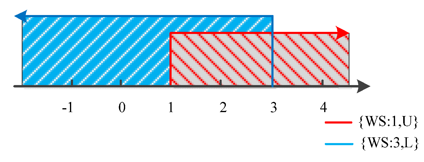
01. //$\beta$ is start_attr in viocfdp 02. for each $\beta \in$ viocfdp do 03.  buffer $\leftarrow$ every $\beta .value$ in viocfdp; 04. end for; 05. if (buffer only L, Not U) 06.  choose max; 07.  result $\leftarrow$ max+”L” 08. else if (buffer only U, Not L) 09.  choose min; 10.  result $\leftarrow$ min+”U”; 11. else if (buffer exists L and U) 12.  judge the location L and U; 13.  do set operation in axis; 14.  get result; 15. end if; 16. return result;

2.3.2. The Convergence and Complexity Analysis of DLA

Since we consider the dynamic process of acquiring the PQ in Section 2.2.2, it is necessary to detect and locate the inconsistent data elements in data instances many times, therefore, the convergence and complexity of detection by the MDS will be analyzed in Section 2.4.2. For a given dependency set, computing the MDS is the key consumption of detecting inconsistent data without considering the detection process by the MDS, and the DLA itself is a loop to obtain the $rcf{d}^p$ continuously. Therefore, it is essential to analysis the convergence and computation complexity of the algorithm.

(1) Convergence analysis

The convergence of DLA means the terminality of the algorithm, which mainly indicates that the process of computing the MDS from the given $cf{d}^p$ must terminate to get new dependency sets. The DLA is convergent for the $cf{d}^p$, and the proof is given below.

Proof 1.

The DLA is convergent for the $cf{d}^p$.

Suppose there are N attributes ($A_1, A_2, A_3,\dots , A_N$) and n $cf{d}^p$($cf{d}_1^P, cf{d}_2^P, cf{d}_3^P,\dots , cf{d}_n^P$) in a data instance, I. Every computing process of acquiring the MDS needs to select an attribute, $A_i$, from the attribute set, A, as the start attribute, and computes the related dependencies to generate m $rcf{d}^p$. The worst case is that all the $n+m$ related $cf{d}^p$(initial $m=0$) of the selected start attribute, $A_i$, are involved in computation, resulting in, at most, [($n+m$)$\times \left(n+m+1\right)]/2$ new dependencies. Because the generation of new dependencies mainly involves set operations and pointers merging (similar to the idea of merging intervals on a number axis), the computational complexity of the two is $\mathrm{O}\left(1\right)$ and $\mathrm{O}\left(n\right)$, respectively. Therefore, it will not fall into endless loops, and the algorithm is convergent to one computation of acquiring the MDS. As a result, the DLA will also be convergent after N traversals. □

(2) Complexity analysis

The time complexity of the DLA depends mainly on two parts: The traversal processes of all attributes and the dynamic domain adjustment.

The traversal processes of all attributes need to select a start attribute, $A_i$, from the attribute set, A, which can be terminated by one traversal and the time complexity is $\mathrm{O}\left(N\right)$.

The complexity of dynamic domain adjustment can also be subdivided into two parts: The generation of the $viocf{d}^P$ and the pointer merging process. The generation of the $viocf{d}^P$ is to do operations with $n+m$ related $cf{d}^p$ and can be obtained by one loop, thus, the time complexity is $\mathrm{O}\left(n+m\right)$. The pointer merging process (i.e., the “union” and “intersection” functions) can complete three steps, the start_attr judgment, forward pointer, L, and backward pointer, U, location identification, through one loop, and the time complexity is also $\mathrm{O}\left(n+m\right)$. In the worst case, the number of newly generated dependencies is $m=n\left(n+1\right)/2$. Therefore, the time complexity of dynamic domain adjustment is $\mathrm{O}\left(2n+2m\right)=\mathrm{O}\left(n^2+3n\right)=\mathrm{O}\left(n^2\right)$.

Accordingly, the time complexity of acquiring MDS is $\mathrm{O}\left(N{n}^2\right)$. The DLA uses the MDS to detect inconsistent data; when comparing with the traditional $cf{d}^p$ based algorithm, the time complexity of the DLA is higher because of new recessive dependencies. The level is determined by the number of the $rcf{d}^p$ and the size of the data instance. The time complexity of detecting inconsistent data elements by the MDS in data instances will be analyzed in Section 2.4.2.

2.4. Inconsistent Data Reparation Algorithm

According to the inconsistent data cleaning framework in Section 2.2, we propose the C-Repair algorithm to repair the inconsistent data detected, which integrates the minimum cost idea and attribute correlation in a data instance, I. To ensure the convergence of the algorithm, we consider a dynamic process to obtain the PQ and set a label, flag, to mark the repaired data elements. Finally, we get the repaired data instance, I’.

2.4.1. Design of Reparation Algorithm

The repair time of a data instance, I, is selected as the repair cost in the C-Repair algorithm. We first sort the inconsistent data elements in the IDS with the minimum cost idea to get the PQ and choose the first element in PQ as the candidate repair data. Then, we obtain the training set, $I_{nv}$, according to the IDS, compute the attribute correlation, SU, and the WDis between the tuple of the candidate repair data and other tuples in $I_{nv}$. At last, we select $n\left(n+1\right)/2, \left(n\ge 2\right)$ class tuples with smaller WDis, and do reparation based on the class tuples. The C-Repair algorithm flow is shown in Algorithm 3.

In Algorithm 3, the L2 to L8 compute the PQ from the IDS using Expression (4), and select a candidate repair data element, β; the L9 to L14 treat the $I_{nv}$ as a training set and learn the correlation SU between the attribute of β and other attributes using Expression (9); the L15 to L21 obtain the WDis between the tuple of β and other tuples in $I_{nv}$ using Expressions (10) and (11); the L22 to L24 select class tuples according to the WDis and repair the data element, β; and the L25 to L28 re-compute the IDS and PQ after a round of reparation to ensure the convergence, and set the label, flag, to ensure every inconsistent data element is repaired at most once.

Algorithm 3. The C-Repair algorithm flow.

Input: data instance I, MDS, IDS Output: repaired result I’

01. for IDS $\ne \varnothing$ do 02.  for ($t_i , A$)$\in$ IDS do 03.   //calculate the count by Formula (4) 04.   α $\leftarrow VioCount\left(t_i , A\right)$; 05.   PQ $\leftarrow$ descending order of α; 06.  end for; 07.  // β is the data element firstly repaired 08.  β $\leftarrow$ first element of PQ; 09.  $I_{nv}\leftarrow$ conflict-free data tuples in I; 10.  //each attribute r.attr in $I_{nv}$ 11.  for r.attr $\in I_{nv}.attr$ do 12.   //calculate the correlation by Formula (9) 13.   SU(β.attr, r.attr); 14.  end for; 15.  //each data tuple $t.t_j$ in $I_{nv}$ 16.  for $t.t_j\in I_{nv}.t_j$ do 17.   //calculate the relative distance by Formula (11) 18.   RDis($\mathsf{\beta }.t_i , t.t_j$); 19.   //calculate the weighted distance by Formula (10) 20.   WDis($\mathsf{\beta }.t_i , t.t_j$); 21.  end for; 22.  buffer $\leftarrow$ ascending order of WDis; 23.  class_tuple $\leftarrow$ choose n(n+1)/2 tuples of buffer; 24.  I’ $\leftarrow$ repair I by class_tuple; 25.  flag $\leftarrow$ β; 26.  IDS $\leftarrow$ recalculate IDS by MDS; 27.  IDS $\leftarrow$ IDS – flag; 28. end for; 29. return I’;

2.4.2. The Convergence and Complexity Analysis of C-Repair

The C-Repair algorithm takes the IDS and MDS, which are output of the DLA, and a data instance, I, as the input, and the output is the repaired data instance, I’. Similar to the DLA, the C-Repair algorithm is also a continuous loop process to gradually repair the inconsistent data, therefore, it is necessary to consider the convergence and complexity of the algorithm.

(1) Convergence analysis

The convergence of the C-Repair algorithm means that the algorithm should terminate and get a stable repair result, I’, after multiple reparation rounds. It can be proved that the C-Repair algorithm is convergent for a data instance, I, with limited tuples.

Proof 2.

The C-Repair algorithm is convergent for a data instance, I, with limited tuples.

Suppose there are M tuples ($t_1, t_2, t_3,\dots , t_M$) and N attributes ($A_1, A_2, A_3,\dots , A_N$) in a data instance, I, and m tuples ($t_1, t_2, t_3,\dots , t_m, m\le M$) in the corresponding conflict-free data instance, $I_{nv}$. The C-Repair algorithm is a loop process to repair the inconsistent data elements based on the IDS; for one reparation round, we need first to select a candidate data element from the $M\times N$ elements according to the IDS and PQ, and then, compute the correlation between the attribute of the candidate repair element and other N − 1 attributes in $I_{nv}$. Finally, we obtain the WDis among tuples based on the correlation, and repair the inconsistent data. In this case, it is convergent to compute the PQ and SU in a data instance with limited tuples, so it is convergent for one round of reparation. In view of multiple reparations, the algorithm can ensure every data element is repaired once at most, because we take a label, flag, to mark the repaired elements. In the worst case, all $M\times N$ data elements in I are inconsistent; at this time, the algorithm will still be convergent due to every reparation round’s convergence, but the loop times will increase. In summary, the C-Repair algorithm is convergent for a data instance, I, with limited tuples. □

(2) Complexity analysis

The C-Repair algorithm needs to select an element as the candidate repair element from the sorted IDS(PQ), and re-compute the IDS after one reparation round. When there are no elements in the IDS, the algorithm ends. Suppose there are $n$ $cf{d}^p$($cf{d}_1^P, cf{d}_2^P, cf{d}_3^P,\dots , cf{d}_n^P$) in the MDS and t data elements in the IDS. For one reparation round, the complexity of the algorithm consists of four parts: Obtaining the PQ, computing the attribute correlation, inconsistent data elements reparation, and re-computing the IDS. There is an execution sequence among these four parts.

To obtain the PQ, we need to compute the violation counts of dependencies, $VioCount$, for every element in the IDS, and computing the $VioCount$ also requires a traversal for every dependency in the MDS, so the time complexity is $\mathrm{O}\left(tn\right)$. When computing the correlation, $SU\left(X,Y\right)$, between attributes, X and Y, we need to first traverse the m tuples in $I_{nv}$ to get the probability, $p\left(x\right)$ and $p\left(y\right),$ of the attributes, X and Y, and compute the corresponding information entropy, H(X) and H(Y), when the time complexity is $\mathrm{O}\left(m\right)$. Then, we traverse every value of the attribute, Y, to get the conditional probability, $p(x|y)$, and compute the correlation, $SU\left(X,Y\right)$, according to Expression (9),when the time complexity is also $\mathrm{O}\left(m\right)$. Therefore, the time complexity of computing the correlation between the candidate repair attribute and other N − 1 attributes is $\mathrm{O}\left(\left(N-1\right)m^2\right)$. The C-Repair algorithm does reparation based on the improved KNN, which computes the WDis between the tuple of the candidate repair element and other tuples in $I_{nv}$ according to the attribute correlation. It should traverse the m tuples and N − 1 attributes in $I_{nv}$, and the time complexity is $\mathrm{O}\left(\left(N-1\right)m\right)$. The purpose of re-computing the IDS is to re-detect the inconsistent data elements based on the MDS of DLA. For a certain $cf{d}^p$, it can be obtained after traversing the related attribute values of every tuple in I, and the time complexity is $\mathrm{O}\left(Mn\right)$.

In summary, for one reparation round, the time complexity can be expressed intuitively as $\mathrm{O}\left(tn+\left(N-1\right)m^2+\left(N-1\right)m+Mn\right)$. In the worst case, all elements in the data instance, I, are inconsistent, that is $t_{max}=MN$, in this case, the time complexity is:

$$O(max(MNn,N{m}^2)$$

For multiple reparations, the maximum repair times can be $t_{max}=MN$, so the time complexity of the C-Repair algorithm is:

$$O(max(M^2{N}^{2}n,M{N}^2{m}^2)$$

(12)

The time complexity in Expression (12) is obtained in the worst case where all elements in I are inconsistent. In an actual data instance, the inconsistent data amount is often small, so the complexity is much smaller than Expression (12).

3. Results

The experiment is divided into two parts in this paper, the detection part and the reparation part, which analyses the validity of the DLA and C-Repair algorithm, respectively. Because it is difficult to get an actual data instance and the contained dependencies at the same time, we use simulation data instance for DLA. However, the C-Repair algorithm is verified both in simulation and actual data instances.

3.1. Experimental Configuration

3.1.1. Experimental Environment

The experiment selects a Core-i7 2.5 GHz processor and 8 GB memory on 64-bit Windows 10 operation system (Hasee, Shenzhen, China). The algorithm is written in Java language, and runs on the Eclipse platform.

3.1.2. Experimental Data Instances

In the detection experiment, we use a simulation data instance (I) to verify the validity of the DLA. Firstly, we specify several dependencies and generate an instance I which satisfies the given dependencies with 1000 consistent data tuples, the staff relation schema in Section 2.1 is selected in I, and the attributes description is shown in Table 1. There are 9 attributes (existing some continuous attributes), 1000 data tuples and 9000 data elements in I, and we can test the applicability of the DLA to continuous attributes.

In reparation experiment, we use both the instance I and the house price forecast instance in Kaggle website (House Prices: Advanced Regression Techniques, HPART) to verify the validity of the C-Repair, and the scale of HPART instance is $1460\times 81$ (1460 tuples and 81 attributes). In unsupervised environment, we randomly generate inconsistent elements in HPART, and compare the repaired results with the original truth values to verify the effectiveness.

In the experiment, in order to reduce the contingency of experimental results, all the data of our experiment are the average results of algorithms running for ten times.

3.1.3. Experimental CFD^Ps

In the experiment, we modified some elements in I to obtain the inconsistent data instance, Ic, based on the given dependencies, and then, detected and repaired the inconsistent data elements in Ic using the DLA and C-Repair algorithm, respectively. By setting multiple inconsistent elements and data tuples in I, the efficiency of different algorithms was compared.

According to the attributes’ description in Table 1, we specified 10 dependencies, which should be satisfied in Ic.

$$cf{d}_1^p:ES=T\to WS\ge 3;cf{d}_6^p:MSy\ge 4500\to MSs=T$$

$$cf{d}_2^p:DM=manager\to MSy\ge 6300;cf{d}_7^p:DM=sale\to MSy\le 6100$$

$$cf{d}_3^p:WS\ge 1\to AGE\ge 19;cf{d}_8^p:WS\ge 2\to MSy\ge 5500$$

$$cf{d}_4^p:WP=branch\#5\to MSy>5000;cf{d}_9^p:WP=branch\#7\to MSy<7000$$

$$cf{d}_5^p:AGE\le 25\to MSs=F;cf{d}_{10}^p:DM=security\to AGE\le 23$$

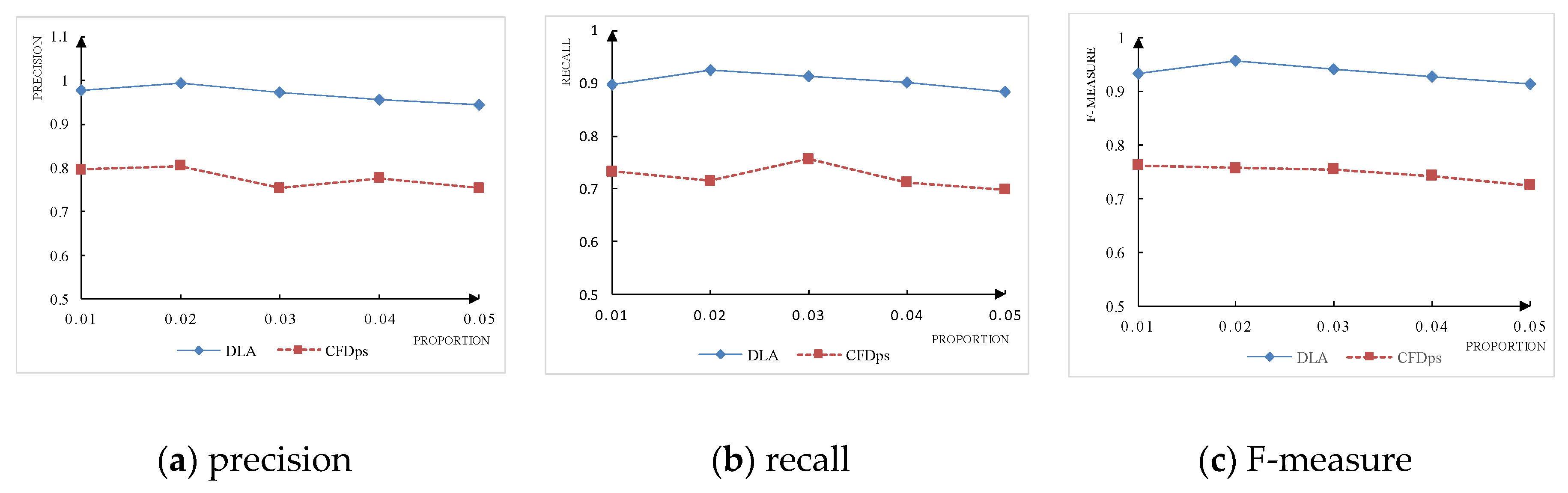
3.2. Experimental Results of the DLA

For inconsistent data detection, the universal method is an algorithm based on the CFD^Ps, which detects the inconsistent elements in data instances according to the given CFD^Ps. We compared the DLA and the CFD^Ps based algorithm in the experiment, and analyzed the accuracy and time-cost of the two algorithms.

3.2.1. Acquiring the MDS

The DLA first computed the recessive dependencies contained in the given dependencies to get the MDS, and detected and located inconsistent elements based on the MDS. According to the DLA flow in Algorithm 1, we obtained six recessive dependencies.

$$rcf{d}_1^p:ES=T\to AGE\ge 19;rcf{d}_4^p:WP=branch\#5\to MSs=T$$

$$rcf{d}_2^p:ES=T\to MSy\ge 5500;rcf{d}_5^p:DM=security\to MSs=F$$

$$rcf{d}_3^p:DM=manager\to MSs=T;rcf{d}_6^p:ES=T\to MSs=T$$

Adding all new $rcf{d}^p$ to the MDS, we eventually obtain the corresponding MDS for the $cf{d}^p$.

$$MDS=\{cf{d}_1^p,cf{d}_2^p,\dots ,cf{d}_{10}^p,rcf{d}_1^p,rcf{d}_2^p,\dots ,rcf{d}_6^p\}$$

3.2.2. Evaluation Indexes

In the inconsistent detection part, we selected two indexes, detection accuracy and time-cost, to compare the DLA with the CFD^Ps based algorithm. The detection accuracy index indicates the detection ability of different algorithms for inconsistent elements, and the time-cost index means the time it takes for algorithms to detect inconsistent data.

(1) Detection Accuracy

In the experiment, we chose three sub-indexes, precision, recall, and F-measure, to measure the detection accuracy of inconsistent data in data instances. Since the precision and recall indexes are conflicting in nature, we used the F-measure, which is the harmonic mean of the precision and recall, to do comprehensive consideration [20] (pp. 1–20). The computing methods of the three sub-indexes are as follows:

$$precision=\frac{sum\_vio\cap sum\_real}{sum\_vio}$$

(13)

$$recall=\frac{sum\_vio\cap sum\_real}{sum\_real}$$

(14)

$$F-measure=\frac{2·precision·recall}{precision+recall}$$

(15)

where $sum\_vio$ and $sum\_real$ represent the detected inconsistent elements and actual inconsistent elements in a data instance, respectively; and $sum\_vio{\displaystyle \cap }sum\_real$ means inconsistent elements correctly detected.

(2) Time-Cost

The time-cost index ($T_c$) means the time of detecting inconsistent elements in a data instance. In this paper, the time-cost of the two algorithms is measured by the system running time.

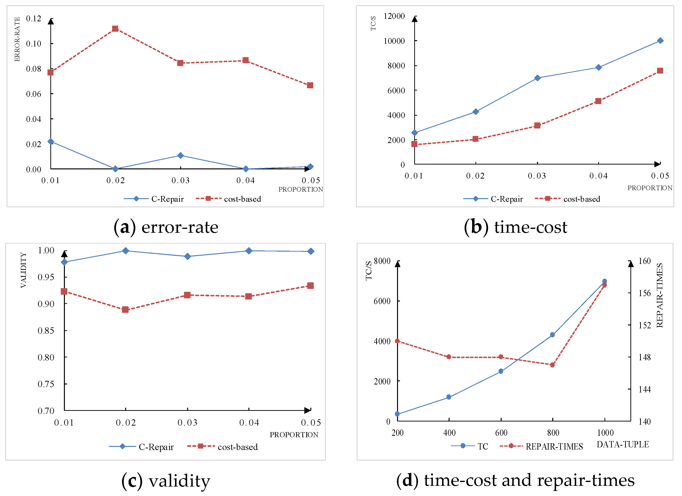
3.2.3. Analysis of the Experimental Results

There were 1000 data tuples, 9 attributes, and 9000 data elements in the original data instance, I, with no missing elements. We obtained the detection accuracy of the DLA and the CFD^Ps based algorithm by setting multiple inconsistent elements (proportion), and the results are shown in Figure 3.

We can see from Figure 3 that the two algorithms have little fluctuation in the detection accuracy of different proportions, and the DLA always performs better than the CFD^Ps based algorithm. However, for a data instance, I, although the DLA performs well in all indexes of the detection accuracy, it is not perfect in all the precision, recall and F-measure index. We think it is caused by errors of the LHS attributes in dependencies.

Next, we analyzed the repair time-cost ($T_c$) of the two algorithms by setting multiple inconsistent data proportions (proportion) and data tuples (data-tuple) in I. The results of the required system time for the two algorithms detection of inconsistent elements are shown in Figure 4.

In the experiment, the $T_c$ was recorded by the average time of 10 runs. As can be seen from the Figure 4a, in the case of fixed data tuples, multiple inconsistent elements’ proportions have small effects on the DLA or the CFD^Ps based algorithm, and Figure 4b shows a sharp increase in the $T_c$ of the two algorithms as data tuples increase in the case of a fixed proportion. In summary, from the experimental results in Figure 4, it is not difficult to see that the $T_c$ of the DLA is always higher than the CFD^Ps based algorithm; that is mainly because the DLA needs get all $rcf{d}^p$ contained in $cf{d}^p$. In this case, the dependencies in the MDS are often more than the given $cf{d}^p$, resulting in a longer detection time of the DLA.

According to the results in Figure 3 and Figure 4, the DLA has a higher time-cost than the CFD^Ps based algorithm, but it has more advantages in detection accuracy. In this paper, we regard this phenomenon as a process of time and accuracy exchange; the difference between detection accuracy and time-cost of the two algorithms was influenced by data tuples and the number of dependencies.

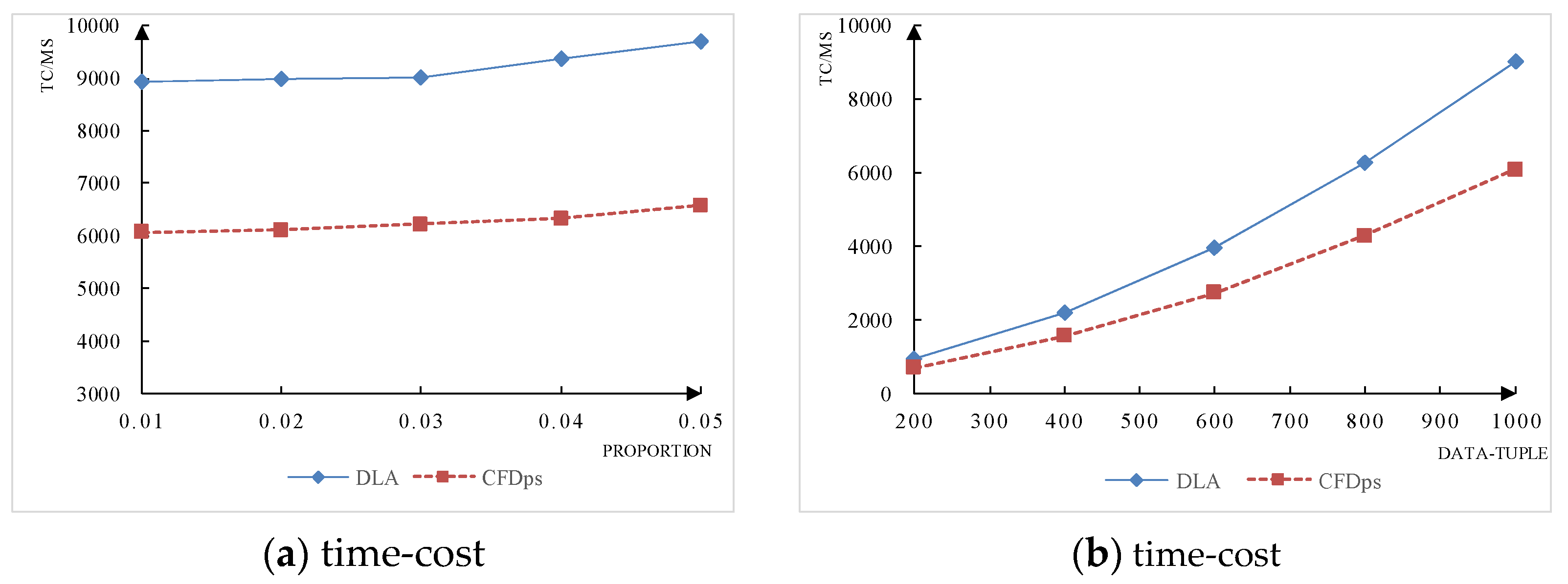
3.3. Experimental Results of the C-Repair

In view of inconsistent elements’ reparation in data instances, we compare the C-Repair with both cost-based and interpolation-based algorithms in the data instance, I, and HPART, and analyze the difference among algorithms in multiple data tuples (data-tuple) and inconsistent elements (proportion).

3.3.1. Evaluation Indexes

In the experiment, we select three indexes, error-rate, time-cost, and validity, to evaluate the pros and cons of C-Repair and two cost-based algorithms in the data instance, I, and select three indexes, validity, satisfaction, and time-cost, to evaluate the pros and cons of C-Repair and two interpolation-based algorithms in the data instance, HPART. Because the C-Repair uses an improved K-NN algorithm combining the attribute correlation and repair cost to do reparation, which selects the most relevant elements in the corresponding conflict-free data instance to replace the original elements in nature, there is no guarantee that the data elements obtained by every reparation will be conflict-free. The error-rate index was used to measure the inconsistent data amount remaining after reparation, and the time-cost index was used to measure the running time of different reparation algorithms, the validity index was used to measure the variation amount of inconsistent elements before and after reparation, and the satisfaction index was used to measure the satisfaction degree of repaired results and initial truth values. The specific computing method is shown as follows.

(1) Error-Rate

Because the repair results of two algorithms cannot always be conflict-free considering the attribute correlation, we introduced the error-rate index, which can be computed as follows, to measure the inconsistent elements remaining in the repaired data instance, I’:

$$error-rate=\frac{{\displaystyle {\sum }_{I\prime }sum\_vio}}{{\displaystyle {\sum }_{I}sum\_vio}}$$

(16)

where ${\displaystyle \sum }_{I^{\prime }}sum\_vio$ means the inconsistent elements amount remaining in a repaired instance, I’; and ${\displaystyle \sum }_{I}sum\_vio$ means the inconsistent elements’ amount in the original instance, I.

(2) Time-Cost

Similar to the time-cost index in Section 3.2, the time-cost ($T_c$) of the reparation algorithm is also described by the system time of the algorithms.

(3) Validity

In the experiment, the validity index is described by the ratio of variation amount in inconsistent elements before and after reparation to the total amount of inconsistent elements in the data instance, I, which can be computed as follows:

$$validity=\frac{{\displaystyle {\sum }_{I}sum\_vio}-{\displaystyle {\sum }_{I\prime }sum\_vio}}{{\displaystyle {\sum }_{I}sum\_vio}}$$

(17)

where ${\displaystyle \sum }_{I}sum\_vio$ means the inconsistent elements amount in the original instance; and ${\displaystyle \sum }_{I^{\prime }}sum\_vio$ means the inconsistent elements’ amount remaining in the repaired instance.

(4) Satisfaction

In inconsistent data reparation, different algorithms always have different repaired values, although all of them may satisfy the given dependency, and there is a gap between them and truth values. In this case, we measured the quality of different repaired values by comparing relative distances between repaired values and corresponding truth values:

$$satisfaction=1-\frac{{\displaystyle {\sum }_n\frac{Dis(repaired,truth)}{Max(repaired,truth)}}}{n}$$

(18)

where $Dis\left(repaired,truth\right)$ means the distance between repaired values and the corresponding truth values, which was measured by the Euclidean distance and edit distance for the numeric attributes and other types, respectively. The $Max\left(repaired,truth\right)$ indicates the larger one between repaired values and truth values, which was measured by the numeric size and string length for the numeric attributes and other types, respectively.

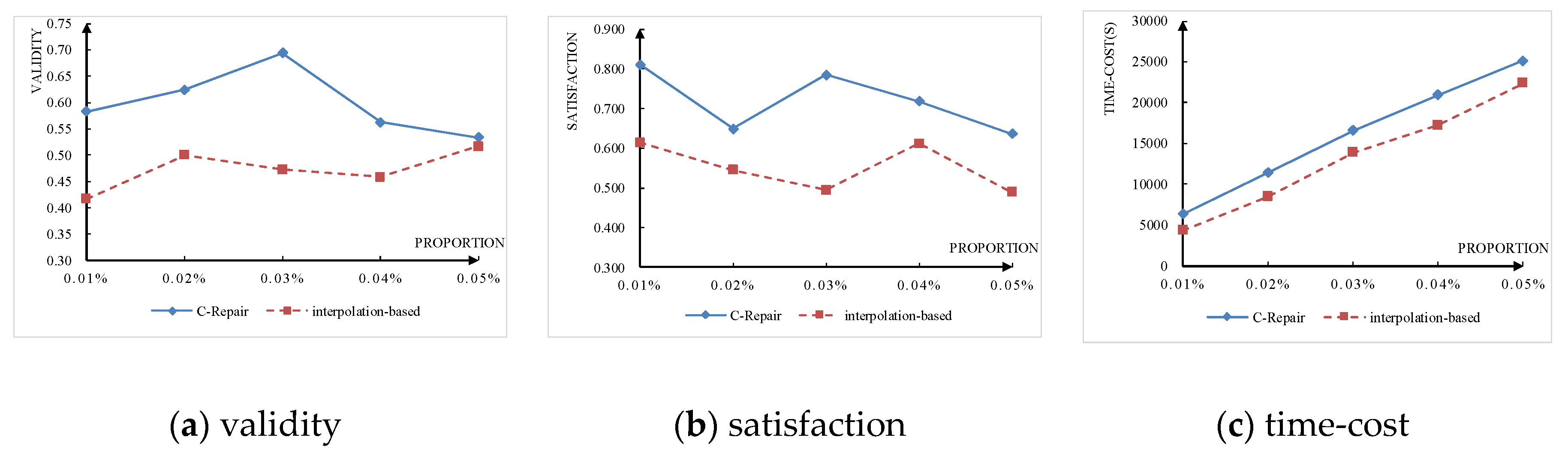
3.3.2. Analysis of the Experimental Results

In the experiment, we first compared the C-Repair algorithm with the cost-based algorithm by setting multiple proportions and data tuples in the data instance, I, and observed the repair capabilities of the two algorithms.

For the data instance, I, with 1000 tuples and 9 attributes, the results of error-rate, time-cost, and validity indexes are shown in Figure 5a–c, respectively, by setting multiple proportions.

To analyze the effect of data tuples on the time-cost ($T_c$) and repair times (repair-times) of the C-Repair algorithm, we set multiple tuples to do the experiment with the fixed inconsistent elements amount (proportion = 0.03), and the results are shown in Figure 5d.

As we can see from Figure 5a–c, although every reparation round of the C-Repair algorithm cannot guarantee a conflict-free result, there were few inconsistent data elements after reparation, and even in the experiment, the repaired data instance, I’, is completely conflict-free many times. We think this is due to a re-computing of the PQ after every reparation round. In Figure 5a–c, the C-Repair algorithm outperforms the cost-based algorithm in both error-rate and validity indexes, but the time-cost is relatively large.

In Figure 5d, we changed the data tuples to observe the $T_c$ and repair-times of the C-Repair algorithm with the fixed proportion. It is not difficult to see that the $T_c$ increased sharply as the data tuples increases, but the repair times were basically stable for the fixed proportion.

For the HPART instance, we compared the C-Repair with the interpolation-based algorithm by setting multiple proportions to observe the repair capabilities of two algorithms.

We set the inconsistent proportions to 0.01%, 0.02%, 0.03%, 0.04%, and 0.05% in the HPART, and the results of the validity, satisfaction, and time-cost indexes are shown in Figure 6a–c, respectively.

From the results in Figure 6a,b, we can see that the validity and satisfaction of the C-Repair algorithm is always higher than the interpolation-based algorithm with the inconsistent proportion change in the HPART instance. In other words, the C-Repair can ensure better results compared with the interpolation-based algorithm, and has less inconsistent data remaining and closer distance between the repaired results and initial truth values. From the results in Figure 6c the time-cost of the two algorithms increases dramatically, and the C-Repair is always higher.

In the experiment, there are two reasons why the C-Repair always has a higher time-cost: (1) We need a high time-cost to learn the correlation from the corresponding $I_{nv}$ because of large data tuples; and (2) we need to compute the WDis between each tuple in $I_{nv}$ and the candidate element to select class tuples; in this case, the time-cost can be high too. In big data, we should make some improvements to satisfy data sets with a huge scale, and it may be a good idea to divide the origin data set into blocks. However, it is worth considering how to divide blocks to improve the time efficiency on the basis of guaranteeing the repair ability.

Combining the results of Figure 5 and Figure 6, we can find that, although the C-Repair can perform better in validity and satisfaction indexes compared with the interpolation-based algorithm in the HPART instance, it is hard to obtain such good results of the simulated instance, I. That is because, unlike the MDS in the simulated instance, I, the truth value of every inconsistent element is unique in the HPART instance. In this case, the repaired results only need to satisfy the MDS of instance, I, to achieve our repair purpose, but a perfect repair result in the HPART instance must be exactly the same as the initial truth value.

4. Discussion

For the inconsistent data cleaning in data instances, we propose the DLA and C-Repair to do detection and reparation, respectively. From the results in Section 3.2, the DLA has a higher detection accuracy and completeness than the traditional dependency-based detection algorithm (CFDs and CFD^Ps), so we think it is feasible to detect inconsistent elements by finding the MDS from given dependency sets. However, the DLA cannot perform perfectly on either the precision or recall index; that is, it cannot detect all inconsistent elements in data instances. We hold the opinion that this may be due to some errors on the LHS attributes of given dependencies, making such inconsistent errors unable to be detected by the MDS, which is also the limitation of DLA. From the results in Section 3.3, the C-Repair algorithm performs better than the cost-based and interpolation-based algorithm in the error-rate, validity, and satisfaction indexes in both simulated data instance, I and HPART. In this case, we think it is feasible to do reparation based on the attributes correlation in an unsupervised environment.

The reason why the DLA performance is better in inconsistent data detection is that it can find recessive dependencies to enlarge the dependency amount, so the detection accuracy and completeness can be improved accordingly. When repairing, there is always a certain correlation among attributes in actual data sets, and the data is not a random occurrence, so we can obtain better results by learning the correlation to guide our repair using the symmetric uncertainty method. Moreover, the C-Repair is an unsupervised repair algorithm without manual intervention, which is also a feature and advantage of the algorithm.

Meanwhile, we find two interesting phenomena in the experiment: (1) The C-Repair algorithm considers the correlation among attributes, and the repair results select the most relevant elements from the corresponding conflict-free instance, instead of directly modifying the values to satisfy the dependencies. Therefore, there may still be a small number of inconsistent elements in the repaired instance, I’. However, when we do experiments on the simulated instance, we get so many consistent results; and (2) the C-Repair can perform better on the simulated instance, I, than the HPART, which may be the unique truth value for every inconsistent element in the HPART instance. The repair results only need to satisfy the MDS in instance, I, which reduces the requirements.

However, both the DLA and C-Repair have a higher time-cost while improving the detection accuracy and repair ability, especially the C-Repair. So, how to reduce the time complexity of two algorithms while maintaining the detection and reparation ability is a problem worth considering. The subsequent research will explore the following three aspects:

(1)

Because dependencies in data instances are not always specified in advance, we may improve the applicability of the DLA through some data mining techniques (i.e., association rules mining [21] (pp. 54–69) and frequent pattern mining [22] (pp. 104–114)), which can obtain dependencies automatically;

(2)

exploring whether we can reduce the time complexity of two algorithms while keeping the detection and reparation ability, which means they can be applied to big data and improves the ability of DLA algorithm to LHS attribute errors; and

(3)

in an unsupervised environment, can the C-Repair algorithm, which integrates the minimum cost idea and attribute correlation, be applied to other data quality problems, such as missing data filling [23] (pp. 157–166) and inaccurate data correction [24] (pp. 230–234).

5. Conclusions

The main achievements of this paper are to propose a data cleaning framework for inconsistent elements and two detection and repair algorithms, DLA and C-Repair. From the experimental results, the DLA can improve the detection accuracy and completeness compared with the dependency-based algorithm, while the C-Repair uses unsupervised machine learning to obtain the correlation among attributes, and gets the most relevant repair results under minimal repair times. Compared with the cost-based and interpolation-based algorithm, the C-Repair performs better in error-rate, validity, and satisfaction indexes, and does not require any manual intervention, so it has a certain applicability in unsupervised cleaning, but also provides a method that can be referenced by other data quality problems.

References

1. Fan, W. Data Quality: From Theory to Practice. ACM SIGMOD Rec. 2015, 44, 7–18. [Google Scholar] [CrossRef]
2. Tu, S.; Huang, M. Scalable Functional Dependencies Discovery from Big Data. In Proceedings of the IEEE Second International Conference on Multimedia Big Data, Taipei, Taiwan, 20–22 April 2016; pp. 426–431. [Google Scholar]
3. Zhou, J.; Diao, X.; Cao, J.; Pan, Z. An Optimization Strategy for CFDMiner: An Algorithm of Discovering Constant Conditional Functional Dependencies. IEICE Trans. Inf. Syst. 2016, E99-D, 537–540. [Google Scholar] [CrossRef]
4. Ma, S.; Duan, L.; Fan, W.; Hu, C.; Chen, W. Extending Conditional Dependencies with Built-in Predicates. IEEE Trans. Knowl. Data Eng. 2015, 27, 3274–3288. [Google Scholar] [CrossRef]
5. Liu, X.-L.; Li, J.-Z. Consistent Estimation of Query Result in Inconsistent Data. Chin. J. Comput. 2015, 38, 1727–1738. [Google Scholar]
6. Parisi, F.; Grant., J. On repairing and querying inconsistent probabilistic spatio-temporal databases. Int. J. Approx. Reason. 2017, 84, 41–74. [Google Scholar] [CrossRef]
7. Bohannon, P.; Fan, W.; Flaster, M.; Rastogi, R. A cost-based model and effective heuristic for repairing constraints by value modification. In Proceedings of the ACM SIGMOD International Conference on Management of Data, Baltimore, MD, USA, 14–16 June 2005; pp. 143–154. [Google Scholar]
8. Brisaboa, N.R.; Rodríguez, M.A.; Seco, D.; Troncoso, R.A. Rank-based strategies for cleaning inconsistent spatial databases. Int. J. Geogr. Inf. Sci. 2015, 29, 280–304. [Google Scholar] [CrossRef]
9. Bai, L.; Shao, Z.; Lin, Z.; Cheng, S. Fixing inconsistencies of fuzzy spatiotemporal XML data. Appl. Intell. 2017, 1–19. [Google Scholar] [CrossRef]
10. Liu, B.; C, M.; Zhou, X. Study on Data Repair and Consistency Query Processing. Comput. Sci. 2016, 43, 232–236, 241. [Google Scholar]
11. Arieli, O.; Zamansky, A. A Graded Approach to Database Repair by Context-Aware Distance Semantics; Elsevier North-Holland, Inc.: Amsterdam, The Netherlands, 2016. [Google Scholar] [CrossRef]
12. Xu, Y.; Li, Z.; Chen, Q.; Zhong, P. Repairing Inconsistent Relational Data Based on Possible Word Model. J. Softw. 2016, 27, 1685–1699. [Google Scholar]
13. Liu, B.; Liu, H. Data consistency repair method for enterprise information integration. Comput. Integr. Manuf. Syst. 2013, 10, 2664–2669. [Google Scholar]
14. Kim, J.; Jang, G.J.; Lee, M. Investigation of the Efficiency of Unsupervised Learning for Multi-task Classification in Convolutional Neural Network. In Neural Information Processing; Springer International Publishing: New York, NY, USA, 2016; pp. 547–554. ISSN 0302-9743. [Google Scholar]
15. Scholtus, S. A generalized Fellegi-Holt paradigm for automatic error localization. Surv. Methodol. 2016, 42, 1–18. [Google Scholar]
16. Zhang, C.; Diao, Y. Conditional functional dependency discovery and data repair based on decision tree. In Proceedings of the International Conference on Fuzzy Systems and Knowledge Discovery, Changsha, China, 13–15 August 2016; pp. 864–868. [Google Scholar]
17. Cao, J.; Diao, X. Introduction to Data Quality; National Defense Industry Press: Beijing, China, 2017; pp. 69–71. ISBN 9787118114058. [Google Scholar]
18. Le, H.T.; Urruty, T.; Gbèhounou, S.; Lecellier, F.; Martinet, J.; Fernandez-Maloigne, C. Improving retrieval framework using information gain models. Signal Image Video Process. 2017, 11, 1–8. [Google Scholar] [CrossRef]
19. Ye, M.; Gao, L.; Wu, C.; Wan, C. Informative Gene Selection Method Based on Symmetric Uncertainly and SVM Recursive Feature Elimination. Pattern Recognit. Artif. Intell. 2017, 30, 429–438. [Google Scholar]
20. Ahmad, H.A.; Wang, H. An effective weighted rule-based method for entity resolution. Distrib. Parallel Databases 2018, 36, 593–612. [Google Scholar] [CrossRef]
21. Martin, D.; Rosete, A.; Alcala-Fdez, J.; Herrera, F. A New Multiobjective Evolutionary Algorithm for Mining a Reduced Set of Interesting Positive and Negative Quantitative Association Rules. IEEE Trans. Evol. Comput. 2014, 18, 54–69. [Google Scholar] [CrossRef]
22. Zhang, X.J.; Wang, M.; Meng, X.F. An Accurate Method for Mining top-k Frequent Pattern Under Differential Privacy. J. Comput. Res. Dev. 2014, 104–114. [Google Scholar]
23. Pedersen, A.B.; Mikkelsen, E.M.; Croninfenton, D.; Kristensen, N.R.; Pham, T.M.; Pedersen, L.; Petersen, I. Missing data and multiple imputation in clinical epidemiological research. Clin. Epidemiol. 2017, 9, 157–166. [Google Scholar] [CrossRef] [PubMed]
24. Diao, Y.; Liu, K.Y.; Meng, X.; Ye, X.; He, K. A Big Data Online Cleaning Algorithm Based on Dynamic Outlier Detection. In Proceedings of the International Conference on Cyber-Enabled Distributed Computing and Knowledge Discovery, Nanjing, China, 12–14 October 2015; pp. 230–234. [Google Scholar]
Figure 1. Inconsistent data detection and reparation framework.
Symmetry 10 00516 g001
Figure 2. Pointer merging processes of the WS attribute.
Symmetry 10 00516 g002
Figure 3. The effect of different proportions on detection precision (the (ac) are all conducted in the instance, I, with 1000 data tuples).
Symmetry 10 00516 g003
Figure 4. Time cost experimental results (the experiment is conducted in the instance, I, the (a) with data-tuple = 1000 and the (b) with proportion = 0.03).
Symmetry 10 00516 g004
Figure 5. Experimental results of two algorithms in I (the (ac) are all conducted with data-tuple = 1000 and the (d) with proportion = 0.03).
Symmetry 10 00516 g005
Figure 6. Experimental results of two algorithms in HPART instance (the (ac) are all conducted in HPART instance with 1460 tuples and 81 attributes).
Symmetry 10 00516 g006