Invariant Graph Partition Comparison Measures

Abstract

Symmetric graphs have non-trivial automorphism groups. This article starts with the proof that all partition comparison measures we have found in the literature fail on symmetric graphs, because they are not invariant with regard to the graph automorphisms. By the construction of a pseudometric space of equivalence classes of permutations and with Hausdorff’s and von Neumann’s methods of constructing invariant measures on the space of equivalence classes, we design three different families of invariant measures, and we present two types of invariance proofs. Last, but not least, we provide algorithms for computing invariant partition comparison measures as pseudometrics on the partition space. When combining an invariant partition comparison measure with its classical counterpart, the decomposition of the measure into a structural difference and a difference contributed by the group automorphism is derived.

1. Introduction

Partition comparison measures are routinely used in a variety of tasks in cluster analysis: finding the proper number of clusters, assessing the stability and robustness of solutions of cluster algorithms, comparing different solutions of randomized cluster algorithms or comparing optimal solutions of different cluster algorithms in benchmarks [1], or in competitions like the 10th DIMACS graph-clustering challenge [2]. Their development has been for more than a century an active area of research in statistics, data analysis and machine learning. One of the oldest and still very well-known measure is the one of Jaccard [3]; more recent approaches were by Horta and Campello [4] and Romano et al. [5]. For an overview of many of these measures, see Appendix B. Besides the need to compare clustering partitions, there is an ongoing discussion of what actually are the best clusters [6,7]. Another problem often addressed is how to measure cluster validity [8,9].

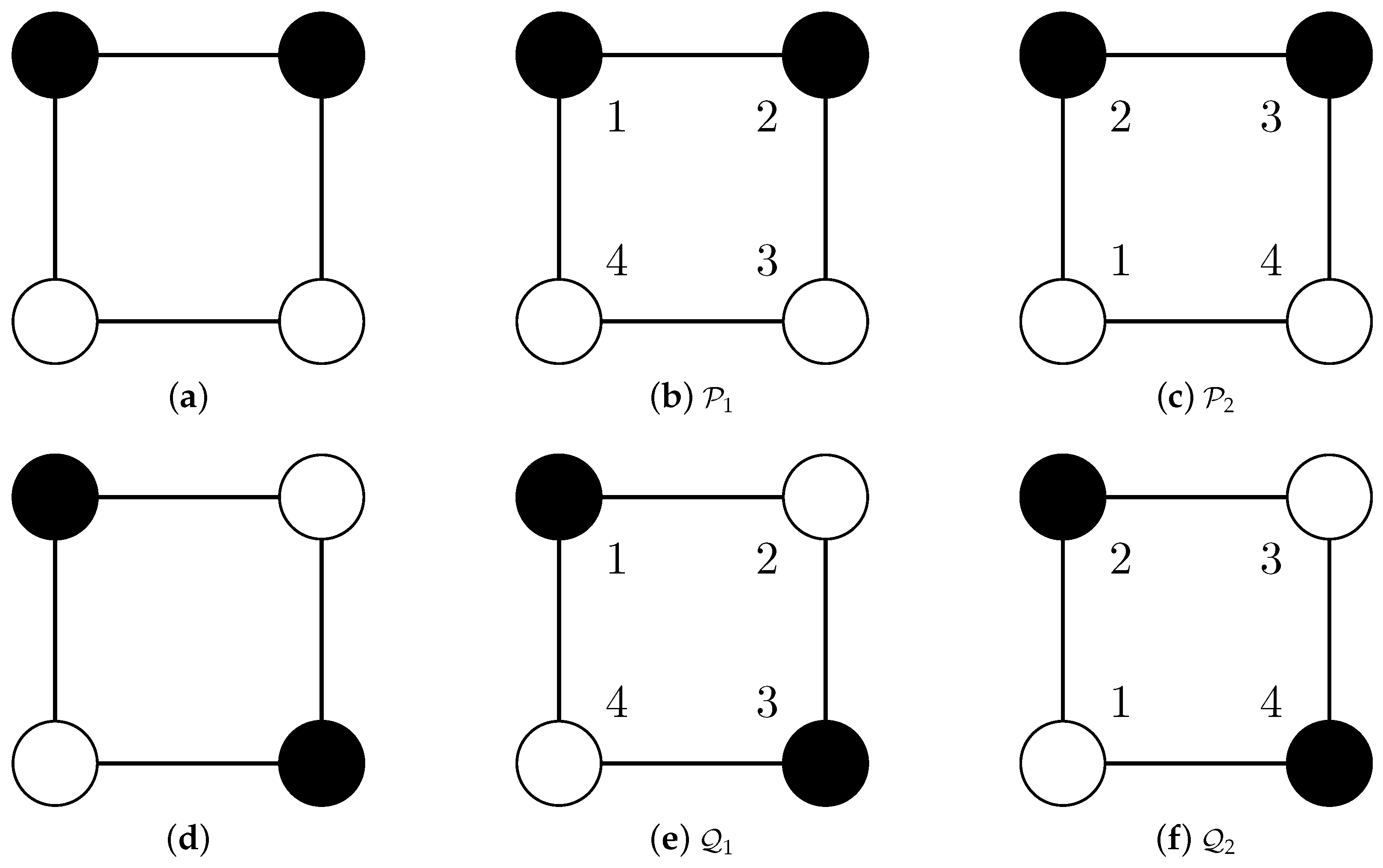
However, the comparison of graph partitions leads to new challenges because of the need to handle graph automorphisms properly. The following small example shows that standard partition comparison measures have unexpected results when applied to graph partitions: in Figure 1, we show two different ways of partitioning the cycle graph $C_4$ (Figure 1a,d). Partitioning means grouping the nodes into non-overlapping clusters. The nodes are arbitrarily labeled with 1 to 4 (Figure 1b,e), and then, there are four possibilities of relabeling the nodes so that the edges stay the same. One possibility is relabeling 1 by 2, 2 by 3, 3 by 4 and 4 by 1, and the images resulting from this relabeling are shown in Figure 1c,f. The relabeling corresponds to a counterclockwise rotation of the graph by 90°, and formal details are given in Section 2. The effects of this relabeling on the partitions ${\mathcal{P}}_1$ and ${\mathcal{Q}}_1$ are different:

• Partition ${\mathcal{P}}_1=\left\{\{1,2\},\{3,4\}\right\}$ is mapped to the structurally equivalent partition ${\mathcal{P}}_2=\left\{\{1,4\},\{2,3\}\right\}$.
• Partition ${\mathcal{Q}}_1=\left\{\{1,3\},\{2,4\}\right\}$ is mapped to the identical partition ${\mathcal{Q}}_2$.

Table 1. The Rand index is $RI=\frac{N_{11}+N_{00}}{N_{11}+N_{10}+N_{01}+N_{00}}$. $N_{11}$ indicates the number of nodes that are in both partitions together in a cluster; $N_{10}$ and $N_{01}$ are the number of nodes that are together in a cluster in one partition, but not in the other; and $N_{00}$ are the number of nodes that are in both partitions in different clusters. See Appendix B for the formal definitions. Partitions ${\mathcal{P}}_1$ and ${\mathcal{P}}_2$ are equivalent (yet not equal, denoted “∼”), and partitions ${\mathcal{Q}}_1$ and ${\mathcal{Q}}_2$ are identical (thus, also equivalent, denoted “=”). However, the comparison of the structurally different partitions (denoted “≠”) ${\mathcal{P}}_i$ and ${\mathcal{Q}}_j$ yields the same result as the comparison between the equivalent partitions ${\mathcal{P}}_1$ and ${\mathcal{P}}_2$. This makes the recognition of structural differences impossible.

Case	Compared Partitions	Relation	${\mathit{N}}_{11}$	${\mathit{N}}_{10}$	${\mathit{N}}_{01}$	${\mathit{N}}_{00}$	RI
1	${\mathcal{P}}_1,{\mathcal{P}}_1$	=	2	0	0	4	1
2	${\mathcal{P}}_2,{\mathcal{P}}_2$	=	2	0	0	4	1
3	${\mathcal{Q}}_1,{\mathcal{Q}}_1$ or ${\mathcal{Q}}_1,{\mathcal{Q}}_2$ or ${\mathcal{Q}}_2,{\mathcal{Q}}_2$	=	2	0	0	4	1
4	${\mathcal{P}}_1,{\mathcal{Q}}_1$ or ${\mathcal{P}}_1,{\mathcal{Q}}_2$	≠	0	2	2	2	$\frac{1}{3}$
5	${\mathcal{P}}_2,{\mathcal{Q}}_1$ or ${\mathcal{P}}_2,{\mathcal{Q}}_2$	≠	0	2	2	2	$\frac{1}{3}$
6	${\mathcal{P}}_1,{\mathcal{P}}_2$	∼	0	2	2	2	$\frac{1}{3}$

illustrates the failure of partition comparison measures (here, the Rand Index (RI)) to recognize structural differences:

• Because ${\mathcal{P}}_1$ and ${\mathcal{P}}_2$ are structurally equivalent, the RI should be one (as for Cases 1, 2 and 3) instead of $1/3$.
• Comparisons of structurally different different partitions (Cases 4 and 5) and comparisons of structurally equivalent partitions (Case 6) should not result in the same value.

One may argue that graphs in real applications contain symmetries only rarely. However, recent investigations of graph symmetries in real graph datasets show that a non-negligible proportion of these graphs contain symmetries. MacArthur et al. [10] state that “a certain degree of symmetry is also ubiquitous in complex systems” [10] (p. 3525). Their study includes a small number of biological, technological and social networks. In addition, Darga et al. [11] studied automorphism groups in very large sparse graphs (circuits, road networks and the Internet router network), with up to five million nodes with eight million links with execution times below 10 s. Katebi et al. [12] reported symmetries in 268 of 432 benchmark graphs. A recent large-scale study conducted by the authors of this article for approximately 1700 real-world graphs revealed that about three quarters of these graphs contain symmetries [13].

The rather frequent occurrence of symmetries in graphs and the obvious deficiencies of classic partition comparison measures demonstrated above have motivated our analysis of the effects of graph automorphisms on partition comparison measures.

Our contribution has the following structure: Permutation groups and graph automorphisms are introduced in Section 2. The full automorphism group of the butterfly graph serves as a motivating example for the formal definition of stable partitions, stable with regard to the actions of the automorphism group of a graph. In Section 3, we first provide a definition that captures the property that a measure is invariant with regard to the transformations in an automorphism group. Based on this definition, we first give a simple proof by counterexample for each partition comparison measure in Appendix B, that these measures based on the comparison of two partitions are not invariant to the effects of automorphisms on partitions. The non-existence of partition comparison measures for which the identity and the invariance axioms hold simultaneously is proven subsequently. In Section 4, we construct three families of invariant partition comparison measures by a two-step process: First, we define a pseudometric space by defining equivalence classes of partitions as the orbit of a partition under the automorphism group $Aut\left(G\right)$. Second, the definitions of the invariant counterpart of a partition comparison measure are given: we define them as the computation of the maximum, the minimum and the average of the direct product of the two equivalence classes. The section also contains a proof of the equivalence of several variants of the computation of the invariant measures, which—by exploiting the group properties of $Aut\left(G\right)$—differ in the complexity of the computation. In Section 5, we introduce the decomposition of the measures into a structurally stable and unstable part, as well as upper bounds for instability. In Section 6, we present an application of the decomposition of measures for analyzing partitions of the Karate graph. The article ends with a short discussion, conclusion and outlook in Section 7.

2. Graphs, Permutation Groups and Graph Automorphisms

We consider connected, undirected, unweighted and loop-free graphs. Let $G=(V,E)$ denote a graph where V is a finite set of nodes and E is a set of edges. An edge is represented as $\{u,v\}\in \left\{\{x,y\}\mid (x,y)\in V\times V\wedge x\ne y\right\}$. Nodes adjacent to $u\in V$ (there exists an edge between u and those nodes) are called neighbors. A partition $\mathcal{P}$ of a graph G is a set of subsets $C_i,i=1,\dots ,k$ of V with the usual properties: (i) $C_i\cap C_j=\varnothing (i\ne j)$, (ii) ${\bigcup }_i{C}_i=V$ and (iii) $C_i\ne \varnothing$. Each subset is called a cluster, and it is identified by its labeled nodes.

As a partition quality criterion, we use the well-known modularity measure Q of Newman and Girvan [14] (see Appendix A). It is a popular optimization criterion for unsupervised graph clustering algorithms, which try to partition the nodes of the graph in a way that the connectivity within the clusters is maximized and the number of edges connecting the clusters is minimized. For a fast and efficient randomized state-of-the-art algorithm, see Ovelgönne and Geyer-Schulz [15].

Partitions are compared by comparison measures, which are functions of the form $m:P\left(V\right)\times P\left(V\right)\to \mathbb{R}$ where $P\left(V\right)$ denotes the set of all possible partitions of the set V. A survey of many of these measures is given in Appendix B.

A permutation on V is a bijection $g:V\to V$. We denote permutations by the symbols $f,g$ and h. Each permutation can be written in cycle form: for a permutation with a single cycle of length r, we write $c=(v_1{v}_2\dots v_r)$. c maps $v_i$ to $v_{i+1}(i=1,\dots ,r-1)$, $v_r$ to $v_1$ and leave all other nodes fixed. Permutations with more than one cycle are written as a product of disjoint cycles (i.e., no two cycles have a common element). $\left(v_k\right)$ means that the element $v_k$ remains fixed, and for brevity, these elements are omitted.

Permutations are applied from the right: The image of u under the permutation g is $ug$. The composition of g and h is $h\circ g$, with ∘ being the permutation composition symbol. For brevity, $h\circ g$ is written as $gh$, so that $u\left(gh\right)=\left(ug\right)h$ holds. Computer scientists call this a postfix notation; in prefix notation, we have $h\left(g\right(u\left)\right)$. Often, we also find $u^g$, which we will use in the following. For k compositions $g\circ g\circ g\circ \dots$, we write $g^k$ and $g^0=id$.

A set of permutation functions forms a permutation group H, if the usual group axioms hold [16]:

• Closure: $\forall g,h\in H:g\circ h\in H$
• Unit element: The identity function $id\in H$ acts as the neutral element: $\forall g\in H:id\circ g=g\circ id=g$
• Inverse element: For any g in H, the inverse permutation function $g^{-1}\in H$ is the inverse of g: $\forall g\in H:g\circ g^{-1}=g^{-1}\circ g=id$
• Associativity: The associative law holds: $\forall f,g,h\in H:f\circ \left(g\circ h\right)=\left(f\circ g\right)\circ h$

If $H_1$ is a subset of H and if $H_1$ is a group, $H_1$ is a subgroup of H (written $H_1\le H$). The set of all permutations of V is denoted by $Sym\left(V\right)$. $Sym\left(V\right)$ is a group, and it is called the symmetric group (see [17]). $Sym\left(V\right)\sim Sym\left(V^{\prime }\right)$ iff $\left|V\right|=\left|V^{\prime }\right|$ with ∼ denoting isomorphism. A generator of a finite permutation group H is a subset of the permutations of H from which all permutations in H can be generated by application of the group axioms [18].

An action of H on V (H acts on V) is called the group action of a set [19] (p. 5):

• $u^{id}=u,\forall u\in V$
• ${\left(u^g\right)}^h=u^{gh},\forall u\in V,\forall g,h\in H$

Groups acting on a set V also act on combinatorial structures defined on V [20] (p. 149), for example the power set $2^V$, the set of all partitions $P\left(V\right)$ or the set of graphs $G\left(V\right)$. We denote combinatorial structures as capital calligraphic letters; in the following, only partitions ($\mathcal{P}$) are of interest because they are the results of graph cluster algorithms. The action of a permutation g on a combinatorial structure is performed by pointwise application of g. For instance, for $\mathcal{P}$, the image of g is ${\mathcal{P}}^g=\{\{u^g\mid u\in C\}\mid C\in \mathcal{P}\}$.

Let H be a permutation group. When H acts on V, a node u is mapped by the elements of H onto other nodes. The set of these images is called the orbit of u under H:

$$u^H=\left\{u^h\mid h\in H\right\}.$$

The group of permutations $H_u$ that fixes u is called the stabilizer of u under H:

$$H_u=\{h\in H\mid u^h=u\}.$$

The orbit stabilizer theorem is given without proof [16]. It links the order of a permutation group with the cardinality of an orbit and the order of the stabilizer:

Theorem 1.

The relation:

$$\left|H\right|=|u^H\left|·\right|H_u|$$

holds.

The action of H on V induces an equivalence relation on the set: for $u_1,u_2\in V$, let $u_1\sim u_2$ iff there exists $h\in H$ so that $u_1=u_2^h$. All elements of an orbit are equivalent, and the orbits of a group partition the set V. An orbit of length one (in terms of set cardinality) is called trivial. Analogously, for a partition $\mathcal{P}$, the definition is:

Definition 1.

The image of the action of H on a partition $\mathcal{P}$ (or the orbit of $\mathcal{P}$ under H) is the set of all equivalent partitions of partition $\mathcal{P}$ under H

$${\mathcal{P}}^H=\left\{{\mathcal{P}}^h\mid h\in H\right\}.$$

A graph automorphism f is a permutation that preserves edges, i.e., $\{u^f,v^f\}\in E\iff \{u,v\}\in E$, $\forall u,v\in V$.

The automorphism group of a graph contains all permutations of vertices that map edges to edges and non-edges to non-edges. The automorphism group of G is defined as:

$$Aut\left(G\right)=\left\{f\in Sym\left(V\right)\mid E^f=E\right\}$$

where $E^f=\left\{\{u^f,v^f\}\mid \{u,v\}\in E\right\}$. Of course, $Aut\left(G\right)\le Sym\left(V\right)$.

Example 1.

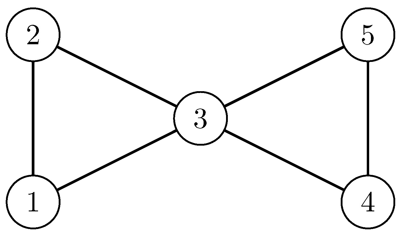
Let $G_{bf}$ be the butterfly graph (Figure 2, e.g., Erdős et al. [21], Burr et al. [22]) whose full automorphism group is given in

Table 2. The full automorphism group $Aut\left(G_{bf}\right)=\left\{id,g_1,\dots ,g_7\right\}$ of the butterfly graph in Figure 2 and its effect on three partitions. Bold partitions are distinct. A possible generator is $\left\{g_1,g_4\right\}$.

Permutation	${\mathcal{P}}_1,\mathit{Q}=0$	${\mathcal{P}}_2,\mathit{Q}=\frac{1}{9}$	${\mathcal{P}}_3,\mathit{Q}=-\frac{1}{18}$
$id=\left(1\right)\left(2\right)\left(3\right)\left(4\right)\left(5\right)$	$\{\mathbf{1},\mathbf{2}\},\left\{\mathbf{3}\right\},\{\mathbf{4},\mathbf{5}\}$	$\{\mathbf{1},\mathbf{2},\mathbf{3}\},\{\mathbf{4},\mathbf{5}\}$	$\{\mathbf{1},\mathbf{2},\mathbf{3},\mathbf{4}\},\left\{\mathbf{5}\right\}$
$g_1=\left(12\right)$	$\{2,1\},\left\{3\right\},\{4,5\}$	$\{2,1,3\},\{4,5\}$	$\{2,1,3,4\},\left\{5\right\}$
$g_2=\left(45\right)$	$\{1,2\},\left\{3\right\},\{5,4\}$	$\{1,2,3\},\{5,4\}$	$\{\mathbf{1},\mathbf{2},\mathbf{3},\mathbf{5}\},\left\{\mathbf{4}\right\}$
$g_3=\left(12\right)\left(45\right)$	$\{2,1\},\left\{3\right\},\{5,4\}$	$\{2,1,3\},\{5,4\}$	$\{2,1,3,5\},\left\{4\right\}$
$g_4=\left(14\right)\left(25\right)$	$\{4,5\},\left\{3\right\},\{1,2\}$	$\{\mathbf{4},\mathbf{5},\mathbf{3}\},\{\mathbf{1},\mathbf{2}\}$	$\{\mathbf{4},\mathbf{5},\mathbf{3},\mathbf{1}\},\left\{\mathbf{2}\right\}$
$g_5=\left(15\right)\left(24\right)$	$\{5,4\},\left\{3\right\},\{2,1\}$	$\{5,4,3\},\{2,1\}$	$\{5,4,3,2\},\left\{1\right\}$
$g_6=\left(1425\right)$	$\{4,5\},\left\{3\right\},\{2,1\}$	$\{4,5,3\},\{2,1\}$	$\{\mathbf{4},\mathbf{5},\mathbf{3},\mathbf{2}\},\left\{\mathbf{1}\right\}$
$g_7=\left(1524\right)$	$\{5,4\},\left\{3\right\},\{1,2\}$	$\{5,4,3\},\{1,2\}$	$\{5,4,3,1\},\left\{2\right\}$

(first column). The permutation $\left(25\right)$ is not an automorphism, because it does not preserve the edges from 1 to 2 and from 5 to 4. The butterfly graph has the two orbits $\{1,2,4,5\}$ and $\left\{3\right\}$. The group $H=\{id,g_1,g_2,g_3\}$ is a subgroup of $Aut\left(G_{bf}\right)$.

Definition 2.

Let $G=(V,E)$ be a graph. A partition $\mathcal{P}$ is called stable, if $|{\mathcal{P}}^{Aut\left(G\right)}|=1$, otherwise it is called unstable.

Stability here means that the automorphism group of the graph does not affect the given partition by tearing apart clusters.

Example 2.

Only ${\mathcal{P}}_1$ in Table 2 is stable because its orbit is trivial. The two modularity optimal partitions (e.g., ${\mathcal{P}}_2^{id}$ and ${\mathcal{P}}_2^{g_4}$) are not stable because $|{\mathcal{P}}_2^{Aut\left(G_{bf}\right)}|=2$. Furthermore, $|{\mathcal{P}}_3^{Aut\left(G_{bf}\right)}|=4$.

For the evaluation of graph clustering solutions, the effects of graph automorphisms on graph partitions are of considerable importance:

• Automorphisms may lead to multiple equivalent optimal solutions as the butterfly graph shows (${\mathcal{P}}_2^{id}$ and ${\mathcal{P}}_2^{g_4}$ in Table 2).
• Partition comparison measures are not invariant with regard to automorphisms, as we show in Section 3.

3. Graph Partition Comparison Measures Are Not Invariant

When comparing graph partitions, a natural requirement is that the partition comparison measure is invariant under automorphism.

Definition 3.

A partition comparison measure $m:P\left(V\right)\times P\left(V\right)\to \mathbb{R}$ is invariant under automorphism, if:

$$m(\mathcal{P},\mathcal{Q})=m(\tilde{\mathcal{P}},\tilde{\mathcal{Q}})$$

for all $\mathcal{P},\mathcal{Q}\in P\left(V\right)$ and $\tilde{\mathcal{P}}\in {\mathcal{P}}^{Aut\left(G\right)}$, $\tilde{\mathcal{Q}}\in {\mathcal{Q}}^{Aut\left(G\right)}$.

Observe that if $\mathcal{Q}\in {\mathcal{P}}^{Aut\left(G\right)}$, then such a measure m cannot distinguish between $\mathcal{P}$ and $\mathcal{Q}$, since $m(\mathcal{P},\mathcal{Q})=m(\mathcal{P},\mathcal{P})$ by definition.

However, unfortunately, as we show in the rest of this section, such a partition comparison measure does not exist. In the following, we present two proofs of this fact, which differ both in their level of generality and sophistication.

3.1. Variant 1: Construction of a Counterexample

Theorem 2.

The measures for comparing partitions defined in Appendix B do not fulfill Definition 3 in general.

Proof. 

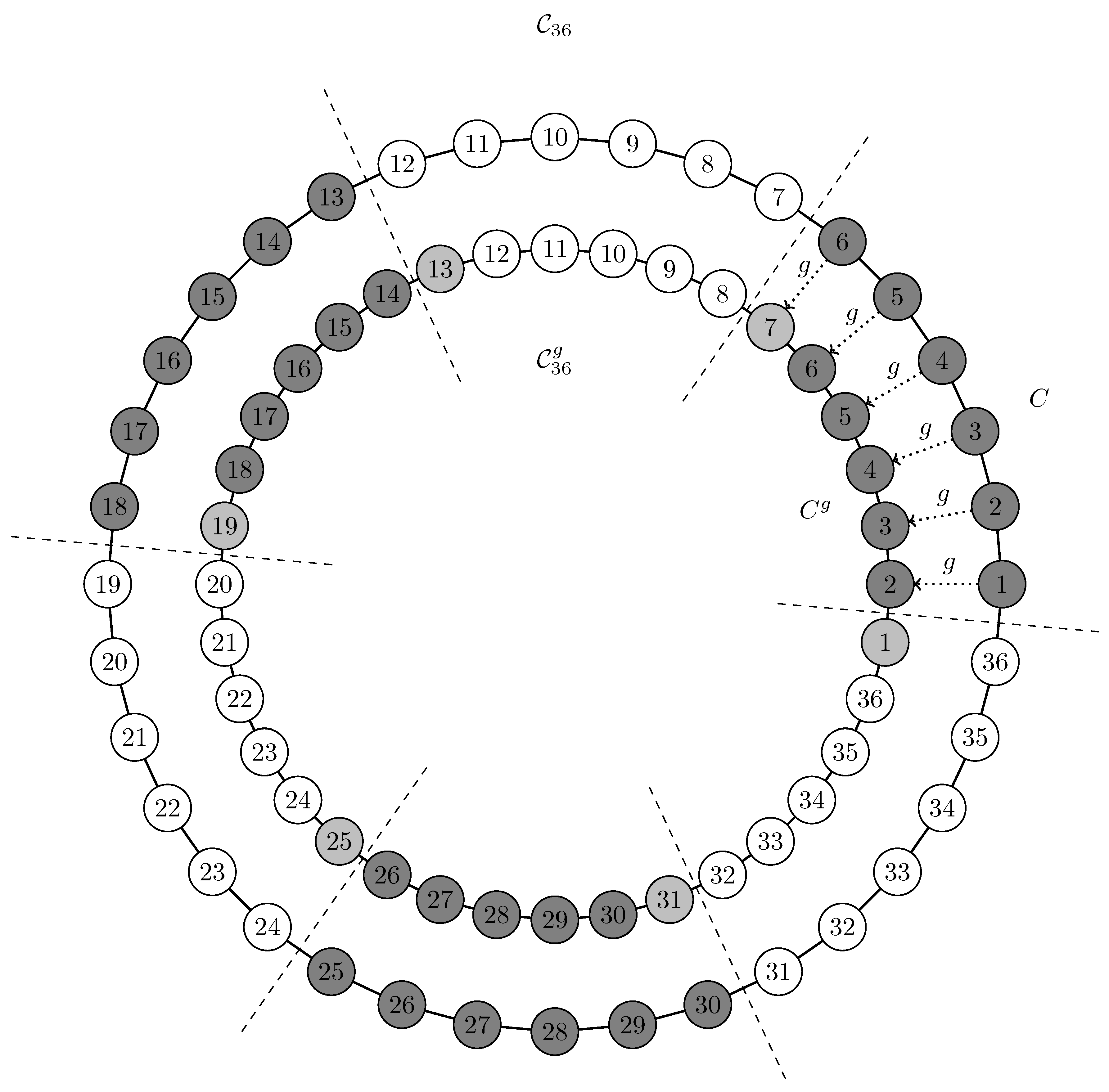
We choose the cycle graph $C_{36}$ and compute all modularity maximal partitions with $Q=2/3$. Each of these six partitions has six clusters, and each of these clusters consists of a chain of six nodes (see Figure 3).

Clearly, since all partitions are equivalent, an invariant partition comparison measure should identify them as equivalent:

$$m({\mathcal{P}}_0,{\mathcal{P}}_0^{g^0})=\dots =m({\mathcal{P}}_0,{\mathcal{P}}_0^{g^5})$$

(1)

Computing $m({\mathcal{P}}_0,{\mathcal{P}}_0^{g^k})$ for $k=0,\dots ,5$ produces

Table 3. Comparing the modularity maximizing partitions of the cycle graph $C_{36}$ with modularity $Q=\frac{2}{3}$. The six optimal partitions consist of six clusters (see Figure 3). The number of pairs in the same cluster in both partitions is denoted by $N_{11}$, in different clusters by $N_{00}$ and in the same cluster in one partition, but not in the other, by $N_{01}$ or $N_{10}$. For the definitions of all partition comparison measures, see Appendix B. To compute this table, the R package partitionComparison has been used [23].

Measure	$\mathit{m}({\mathcal{P}}_0,{\mathcal{P}}_0^{{\mathit{g}}^{\mathit{k}}})$ with $\mathit{g}=\left(123\mathit{\dots }3536\right)$ for k:
	0	1	2	3	4	5
	Pair counting measures ($f(N_{11},N_{00},N_{01},N_{10})$; see Table A1 and Table A2)
RI	$1.0$	$0.90476$	$0.84762$	$0.82857$	$0.84762$	$0.90476$
ARI	$1.0$	$$0.61111$$	$0.37778$	$0.3$	$0.37778$	$0.61111$
H	$1.0$	$0.80952$	$0.69524$	$0.65714$	$0.69524$	$0.80952$
CZ	$1.0$	$0.66667$	$0.46667$	$0.4$	$0.46667$	$0.66667$
K	$1.0$	$0.66667$	$0.46667$	$0.4$	$0.46667$	$0.66667$
MC	$1.0$	$0.33333$	$-0.06667$	$-0.2$	$-0.06667$	$0.33333$
P	$1.0$	$0.61111$	$0.37778$	$0.3$	$0.37778$	$0.61111$
WI	$1.0$	$0.66667$	$0.46667$	$0.4$	$0.46667$	$0.66667$
WII	$1.0$	$0.66667$	$0.46667$	$0.4$	$0.46667$	$0.66667$
FM	$1.0$	$0.66667$	$0.46667$	$0.4$	$0.46667$	$0.66667$
$\Gamma$	$1.0$	$0.61111$	$0.37778$	$0.3$	$0.37778$	$0.61111$
SS1	$1.0$	$0.80556$	$0.68889$	$0.65$	$0.68889$	$0.80556$
B1	$1.0$	$0.91383$	$0.87084$	$0.85796$	$0.87084$	$0.91383$
GL	$1.0$	$0.95$	$0.91753$	$0.90625$	$0.91753$	$0.95$
SS2	$1.0$	$0.33333$	$0.17949$	$0.14286$	$0.17949$	$0.33333$
SS3	$1.0$	$0.62963$	$0.42519$	$0.36$	$0.42519$	$0.62963$
RT	$1.0$	$0.82609$	$0.73554$	$0.70732$	$0.73554$	$0.82609$
GK	$1.0$	$0.94286$	$0.79937$	$0.71429$	$0.79937$	$0.94286$
J	$1.0$	$0.5$	$0.30435$	$0.25$	$0.30435$	$0.5$
RV	$1.0$	$0.61039$	$0.37662$	$0.29870$	$0.37662$	$0.61039$
RR	$0.14286$	$0.09524$	$0.06667$	$0.05714$	$0.06667$	$0.09524$
M	$0.0$	12$0.0$	19$2.0$	21$6.0$	19$2.0$	12$0.0$
Mi	$0.0$	$0.81650$	$1.03280$	$1.09545$	$1.03280$	$0.81650$
Pe	$0.00002$	$0.00001$	$0.00001$	$0.00001$	$0.00001$	$0.00001$
B2	$0.12245$	$0.07483$	$0.04626$	$0.03673$	$0.04626$	$0.07483$
LI	2$4.37212$	1$4.89407$	$9.20724$	$7.31163$	$9.20724$	1$4.89407$
NLI	$1.0$	$0.61111$	$0.37778$	$0.3$	$0.37778$	$0.61111$
FMG	$0.94730$	$0.61396$	$0.41396$	$0.34730$	$0.41396$	$0.61396$
	Set-based comparison measures (see Table A3)
LA	$1.0$	$0.83333$	$0.66667$	$0.5$	$0.66667$	$0.83333$
$d_{CE}$	$0.0$	$0.16667$	$0.33333$	$0.5$	$0.33333$	$0.16667$
D	$0.0$	1$2.0$	2$4.0$	3$6.0$	2$4.0$	1$2.0$
	Information theory-based measures (see Table A4)
MI	$1.79176$	$1.34120$	$1.15525$	$1.09861$	$1.15525$	$1.34120$
NMI (max)	$1.0$	$0.74854$	$0.64475$	$0.61315$	$0.64475$	$0.74854$
NMI (min)	$1.0$	$0.74854$	$0.64475$	$0.61315$	$0.64475$	$0.74854$
NMI ($\mathsf{\Sigma }$)	$1.0$	$0.74854$	$0.64475$	$0.61315$	$0.64475$	$0.74854$
VI	$0.0$	$0.90112$	$1.27303$	$1.38629$	$1.27303$	$0.90112$

. Because the values in each row differ (in contrast to the requirements defined by Equation (1)), each row of Table 3 contains the counterexample for the measure used.  □

3.2. Variant 2: Inconsistency of the Identity and the Invariance Axiom

Theorem 3.

Let $G=(V,E)$ be a graph with $\left|V\right|>2$ and nontrivial $Aut\left(G\right)$. For partition comparison measures $m:P\left(V\right)\times P\left(V\right)\to \mathbb{R}$, it is impossible to fulfill jointly the identity axiom $m(\mathcal{P},\mathcal{Q})=c$, if and only if $\mathcal{P}=\mathcal{Q}$ (e.g., for a distance measure $c=0$, for a similarity measure $c=1$, etc.) for all $\mathcal{P},\mathcal{Q}\in P\left(V\right)$ and the axiom of invariance (from Definition 3) $m(\mathcal{P},\mathcal{Q})=c,\forall \mathcal{Q}\in {\mathcal{P}}^{Aut\left(G\right)}$.

Proof. 

• Since $Aut\left(G\right)$ is nontrivial, a nontrivial orbit with at least two different partitions, namely $\mathcal{P}$ and $\mathcal{Q}$, exists because $|{\mathcal{P}}^{Aut\left(G\right)}|>1$. It follows from the invariance axiom that $m(\mathcal{P},\mathcal{Q})=c$.
• The identity axiom implies that it follows from $m(\mathcal{P},\mathcal{Q})=c$ that $\mathcal{P}=\mathcal{Q}$.
• This contradicts the assumption that $\mathcal{P}$ and $\mathcal{Q}$ are different.

 □

4. The Construction of Invariant Measures for Finite Permutation Groups

The purpose of this section is to construct invariant counterparts for most of the partition comparison measures in Appendix B. We proceed in two steps:

• We construct a pseudometric space from the images of the actions of $Aut\left(G\right)$ on partitions in $P\left(V\right)$ (Definition 1).
• We extend the metrics for partition comparison by constructing invariant metrics on the pseudo-metric space of partitions.

4.1. The Construction of the Pseudometric Space of Equivalence Classes of Graph Partitions

We use a variant of the idea of Doob’s concept of a pseudometric space [24] (p. 5). A metric for a space S (with $s,t,u\in S$) is a function $d:S\times S\to {\mathbb{R}}^{+}$ for which the following holds:

• Symmetry: $d(s,t)=d(t,s)$.
• Identity: $d(s,t)=0$ if and only if $s=t$.
• Triangle inequality: $d(s,u)\le d(s,t)+d(t,u)$.

A pseudometric space $(S,d^{\ast })$ relaxes the identity condition to $d^{\ast }(s,s)=0$. The distance between two elements $s_1,s_2$ of an equivalence class $\left[s\right]$ is defined as $d^{\ast }(s_1,s_2)=0$ by Definition 3.

For graphs, S is the finite set of partitions $P\left(V\right)$ and $S^{\ast }$ is the partition of $P\left(V\right)$ into orbits of $Aut\left(G\right)$:

$$S^{\ast }\left(V\right)=P{\left(V\right)}^{Aut\left(G\right)}=\left\{{\mathcal{P}}^{Aut\left(G\right)}\mid \mathcal{P}\in P\left(V\right)\right\}.$$

A partition $\mathcal{P}$ in S corresponds to its orbit ${\mathcal{P}}^{Aut\left(G\right)}$ in $S^{\ast }$. The relations between the spaces used in the following are:

• $(S,d)$ is a metric space with $S=P\left(V\right)$ and with the function $d:P\left(V\right)\times P\left(V\right)\to \mathbb{R}$.
• $(S^{\ast },d^{\ast })$ is a metric space with $S^{\ast }=P{\left(V\right)}^{Aut\left(G\right)}=\{{\mathcal{P}}^{Aut\left(G\right)}\mid \mathcal{P}\in P\left(V\right)\}$ and the function $d^{\ast }$: $P{\left(V\right)}^{Aut\left(G\right)}\times P{\left(V\right)}^{Aut\left(G\right)}\to \mathbb{R}$. We construct three variants of $d^{\ast }$ in Section 4.2.
• $(S,d^{\ast })$ is the pseudometric space with $S=P\left(V\right)$ and with the metric $d^{\ast }$. The partitions in S are mapped to arguments of $d^{\ast }$ by the transformation $ec:P\left(V\right)\to P{\left(V\right)}^{Aut\left(G\right)}$, which is defined as $ec\left(\mathcal{P}\right){\mathcal{P}}^{Aut\left(G\right)}$.

Table 4. The equivalence classes of the pseudometric space $(S,d^{\ast })$ of the butterfly graph (see Figure 2). Classes are grouped by their partition type, which is the corresponding integer partition. k is the number of partitions per type; l is the number of clusters the partitions of a type consists of; ${dia}_{1-RI}$ is the diameter (see Equation (2)) of the equivalence class computed for the distance $d_{RI}$ computed from the Rand Index (RI) by $1-RI$.

	${\mathcal{P}}^{\mathit{Aut}\left(\mathit{G}\right)}$	Q	${dia}_{1-\mathit{RI}}$
	Partition type $(1,1,1,1,1)$, $k=1$, $l=5$
${\mathit{E}}_{\mathbf{1}}$	$\left\{1\right\},\left\{2\right\},\left\{3\right\},\left\{4\right\},\left\{5\right\}$	$-\frac{2}{9}$	$0.0$
	Partition type $(1,1,1,2)$, $k=10$, $l=4$
$E_2$	$\left\{1\right\},\left\{2\right\},\left\{3\right\},\{4,5\}\{1,2\},\left\{3\right\},\left\{4\right\},\left\{5\right\}$	$-\frac{1}{9}$	$0.2$
$E_3$	$\left\{1\right\},\left\{2\right\},\{3,4\},\left\{5\right\}\left\{1\right\},\left\{2\right\},\{3,5\},\left\{4\right\}\left\{1\right\},\{2,3\},\left\{4\right\},\left\{5\right\}$	$-\frac{1}{6}$	$0.2$
	$\{1,3\},\left\{2\right\},\left\{4\right\},\left\{5\right\}$
$E_4$	$\left\{1\right\},\{2,4\},\left\{3\right\},\left\{5\right\}\left\{1\right\},\{2,5\},\left\{3\right\},\left\{4\right\}\{1,4\},\left\{2\right\},\left\{3\right\},\left\{5\right\}$	$-\frac{5}{18}$	$0.2$
	$\{1,5\},\left\{2\right\},\left\{3\right\},\left\{4\right\}$
	Partition type $(1,1,3)$ $k=10$, $l=3$
$E_5$	$\left\{1\right\},\left\{2\right\},\{3,4,5\}\left\{4\right\},\left\{5\right\},\{1,2,3\}$	0	$0.6$
$E_6$	$\left\{1\right\},\left\{3\right\},\{2,4,5\}\left\{3\right\},\left\{5\right\},\{1,2,4\}\left\{3\right\},\left\{4\right\},\{1,2,5\}$	$-\frac{2}{9}$	$0.4$
	$\left\{2\right\},\left\{3\right\},\{1,4,5\}$
$E_7$	$\left\{1\right\},\left\{5\right\},\{2,3,4\}\left\{1\right\},\left\{4\right\},\{2,3,5\}\left\{2\right\},\left\{5\right\},\{1,3,4\}$	$-\frac{1}{6}$	$0.6$
	$\left\{2\right\},\left\{4\right\},\{1,3,5\}$
	Partition type $(1,2,2)$, $k=15$, $l=3$
${\mathit{E}}_{\mathbf{8}}$	$\left\{3\right\},\{1,2\},\{4,5\}$	0	$0.0$
$E_9$	$\left\{3\right\},\{1,4\},\{2,5\}\left\{3\right\},\{1,5\},\{2,4\}$	$-\frac{1}{3}$	$0.4$
$E_{10}$	$\left\{1\right\},\{2,3\},\{4,5\}\left\{5\right\},\{1,2\},\{3,4\}\left\{4\right\},\{1,2\},\{3,5\}$	$-\frac{1}{18}$	$0.4$
	$\left\{2\right\},\{1,3\},\{4,5\}$
$E_{11}$	$\left\{1\right\},\{2,4\},\{3,5\}\left\{1\right\},\{2,5\},\{3,4\}\left\{5\right\},\{1,3\},\{2,4\}$	$-\frac{2}{9}$	$0.4$
	$\left\{4\right\},\{1,3\},\{2,5\}\left\{2\right\},\{1,4\},\{3,5\}\left\{5\right\},\{1,4\},\{2,3\}$
	$\left\{2\right\},\{1,5\},\{3,4\}\left\{4\right\},\{1,5\},\{2,3\}$
	Partition type $(1,4)$, $k=5$, $l=2$
${\mathit{E}}_{\mathbf{12}}$	$\{1,2,4,5\},\left\{3\right\}$	$-\frac{2}{9}$	$0.0$
$E_{13}$	$\{2,3,4,5\},\left\{1\right\}\{1,2,3,4\},\left\{5\right\}\{1,2,3,5\},\left\{4\right\}$	$-\frac{1}{18}$	$0.6$
	$\{1,3,4,5\},\left\{2\right\}$
	Partition type $(2,3)$, $k=10$, $l=2$
$E_{14}$	$\{1,2\},\{3,4,5\}\{4,5\},\{1,2,3\}$	$\frac{1}{9}$	$0.4$
$E_{15}$	$\{3,5\},\{1,2,4\}\{3,4\},\{1,2,5\}\{1,3\},\{2,4,5\}$	$-\frac{1}{6}$	$0.6$
	$\{2,3\},\{1,4,5\}$
$E_{16}$	$\{2,5\},\{1,3,4\}\{2,4\},\{1,3,5\}\{1,4\},\{2,3,5\}$	$-\frac{2}{9}$	$0.6$
	$\{1,5\},\{2,3,4\}$
	Partition type $\left(5\right)$, $k=1$, $l=1$
${\mathit{E}}_{\mathbf{17}}$	$\{1,2,3,4,5\}$	0	$0.0$

illustrates $S^{\ast }$ (the space of equivalence classes) of the pseudometric space $(S,d^{\ast })$ of the butterfly graph (shown in Figure 2). $S^{\ast }$ is the partition of $P\left(\right\{1,2,3,4,5\left\}\right)$ into 17 equivalence classes. Only the four classes $E_1$, $E_8$, $E_{12}$ and $E_{17}$ are stable because they are trivial orbits. The three partitions from Table 2 are contained in the following equivalence classes: ${\mathcal{P}}_1\in E_8$, ${\mathcal{P}}_2\in E_{14}$, and ${\mathcal{P}}_3\in E_{13}$.

4.2. The Construction of Left-Invariant and Additive Measures on the Pseudometric Space of Equivalence Classes of Graph Partitions

In the following, we consider only partition comparison measures, which are distance functions of a metric space. Note that a normalized similarity measure s can be transformed into a distance by the transformation $d=1-s$.

In a pseudometric space $(S,d^{\ast })$, we measure the distance $d^{\ast }(\mathcal{P},\mathcal{Q})$ between equivalence classes (which are sets) of partitions instead of the distance $d(\mathcal{P},\mathcal{Q})$ between partitions. The partitions $\mathcal{P}$ and $\mathcal{Q}$ are formal arguments of $d^{\ast }$, which are expanded to equivalence classes by ${\mathcal{P}}^{Aut\left(G\right)}$ and ${\mathcal{Q}}^{Aut\left(G\right)}$. The standard construction of a distance measure between sets has been developed for the point set topology and is due to Felix Hausdorff [25] (p. 166) and Kazimierz Kuratowski [26] (p. 209). For finite sets, it requires the computation of the distances for all pairs of the direct product of the two sets. Since for finite permutation groups, we deal with distances between two finite sets of partitions, we use the following definitions for the lower and upper measures, respectively. Both definitions have the form of an optimization problem:

$$d_L^{\ast }(\mathcal{P},\mathcal{Q})=\underset{\begin{array}{c}\tilde{\mathcal{P}}\in {\mathcal{P}}^{Aut\left(G\right)},\\ \tilde{\mathcal{Q}}\in {\mathcal{Q}}^{Aut\left(G\right)}\end{array}}{min}d(\tilde{\mathcal{P}},\tilde{\mathcal{Q}})$$

and:

$$d_U^{\ast }(\mathcal{P},\mathcal{Q})=\left\{\begin{array}{cc}0& if{\mathcal{P}}^{Aut\left(G\right)}={\mathcal{Q}}^{Aut\left(G\right)}\\ \underset{\begin{array}{c}\tilde{\mathcal{P}}\in {\mathcal{P}}^{Aut\left(G\right)},\\ \tilde{\mathcal{Q}}\in {\mathcal{Q}}^{Aut\left(G\right)}\end{array}}{max}d(\tilde{\mathcal{P}},\tilde{\mathcal{Q}})& \mathrm{else}\end{array}\right.$$

The diameter of a finite equivalence class of partitions is defined by

$$dia\left(\mathcal{P}\right)=\underset{\begin{array}{c}\tilde{\mathcal{P}}\in {\mathcal{P}}^{Aut\left(G\right)},\\ \tilde{\mathcal{Q}}\in {\mathcal{P}}^{Aut\left(G\right)}\end{array}}{max}d(\tilde{\mathcal{P}},\tilde{\mathcal{Q}}).$$

(2)

The third option of defining a distance between two finite equivalence classes of partitions of taking the average distance is due to John von Neumann [27]:

$$d_{av}^{\ast }(\mathcal{P},\mathcal{Q})=\left\{\begin{array}{cc}0& \mathrm{if}{\mathcal{P}}^{Aut\left(G\right)}={\mathcal{Q}}^{Aut\left(G\right)}\\ \frac{1}{|{\mathcal{P}}^{Aut\left(G\right)}\left|·\right|{\mathcal{Q}}^{Aut\left(G\right)}|}\sum _{\begin{array}{c}\tilde{\mathcal{P}}\in {\mathcal{P}}^{Aut\left(G\right)},\\ \tilde{\mathcal{Q}}\in {\mathcal{Q}}^{Aut\left(G\right)}\end{array}}d(\tilde{\mathcal{P}},\tilde{\mathcal{Q}})& \mathrm{else}\end{array}\right.$$

Note that the definitions for $d_L^{\ast }$, $d_U^{\ast }$ and $d_{av}^{\ast }$ require the computation of the minimal, maximal and average distance of all pairs of the direct product ${\mathcal{P}}^{Aut\left(G\right)}\times {\mathcal{Q}}^{Aut\left(G\right)}$. The computational complexity of this is quadratic in the size of the larger equivalence class.

Posed as a measurement problem, we can instead fix one partition in one of the orbits and measure the minimal, maximal and average distance between all pairs of either the direct product of $\left\{\mathcal{P}\right\}\times {\mathcal{Q}}^{Aut\left(G\right)}$ or $\left\{\mathcal{Q}\right\}\times {\mathcal{P}}^{Aut\left(G\right)}$. The complexity of this is linear in the size of the smaller equivalence class.

Theorems 4 and 5 and their proofs are based on these observations. They are the basis for the development of algorithms for the computation of invariant partition comparison measures of a computational complexity of at most linear order and often of constant order.

Theorem 4.

For all ${\mathcal{P}}^{Aut\left(G\right)}\ne {\mathcal{Q}}^{Aut\left(G\right)}$, the following equations hold:

$$\begin{array}{ccc}\hfill d_L^{\ast }(\mathcal{P},\mathcal{Q})& =\underset{\begin{array}{c}\tilde{\mathcal{P}}\in {\mathcal{P}}^{Aut\left(G\right)},\\ \tilde{\mathcal{Q}}\in {\mathcal{Q}}^{Aut\left(G\right)}\end{array}}{min}d(\tilde{\mathcal{P}},\tilde{\mathcal{Q}})\hfill & =\underset{g,h\in Aut\left(G\right)}{min}d({\mathcal{P}}^h,{\mathcal{Q}}^g)\hfill \\ & =\underset{\tilde{\mathcal{Q}}\in Q^{Aut\left(G\right)}}{min}d(\mathcal{P},\tilde{\mathcal{Q}})\hfill & =\underset{g\in Aut\left(G\right)}{min}d(\mathcal{P},{\mathcal{Q}}^g)\hfill \\ & =\underset{\tilde{\mathcal{P}}\in P^{Aut\left(G\right)}}{min}d(\tilde{\mathcal{P}},\mathcal{Q})\hfill & =\underset{h\in Aut\left(G\right)}{min}d({\mathcal{P}}^h,\mathcal{Q})\hfill \end{array}$$

For ${\mathcal{P}}^{Aut\left(G\right)}\ne {\mathcal{Q}}^{Aut\left(G\right)}$:

$$\begin{array}{ccc}\hfill d_U^{\ast }(\mathcal{P},\mathcal{Q})& =\underset{\begin{array}{c}\tilde{\mathcal{P}}\in {\mathcal{P}}^{Aut\left(G\right)},\\ \tilde{\mathcal{Q}}\in {\mathcal{P}}^{Aut\left(G\right)}\end{array}}{max}d(\tilde{\mathcal{P}},\tilde{\mathcal{Q}})\hfill & =\underset{g,h\in Aut\left(G\right)}{max}d({\mathcal{P}}^h,{\mathcal{Q}}^g)\hfill \\ & =\underset{\tilde{\mathcal{Q}}\in Q^{Aut\left(G\right)}}{max}d(\mathcal{P},\tilde{\mathcal{Q}})\hfill & =\underset{g\in Aut\left(G\right)}{max}d(\mathcal{P},{\mathcal{Q}}^g)\hfill \\ & =\underset{\tilde{\mathcal{P}}\in P^{Aut\left(G\right)}}{max}d(\tilde{\mathcal{P}},\mathcal{Q})\hfill & =\underset{h\in Aut\left(G\right)}{max}d({\mathcal{P}}^h,\mathcal{Q})\hfill \end{array}$$

Proof. 

Let $g,h,f\in Aut\left(G\right)$, $\tilde{\mathcal{P}}\in {\mathcal{P}}^{Aut\left(G\right)}$ and $\tilde{\mathcal{Q}}\in {\mathcal{Q}}^{Aut\left(G\right)}$, that is $\tilde{\mathcal{P}}={\mathcal{P}}^h$ and $\tilde{\mathcal{Q}}={\mathcal{Q}}^g$. Then, since the orbits of both partitions are generated by $Aut\left(G\right)$, the following identities between distances hold:

$$\begin{array}{ccc}\hfill d(\mathcal{P},\tilde{\mathcal{Q}})& =d(\mathcal{P},{\mathcal{Q}}^g)\hfill & =d({\mathcal{P}}^{g^{-1}},\mathcal{Q}),\hfill \\ \hfill d(\tilde{\mathcal{P}},\mathcal{Q})& =d({\mathcal{P}}^h,\mathcal{Q})\hfill & =d(\mathcal{P},{\mathcal{Q}}^{h^{-1}})\hfill \end{array}$$

as well as:

$$d(\tilde{\mathcal{P}},\tilde{\mathcal{Q}})=d({\mathcal{P}}^h,{\mathcal{Q}}^g)=d({\mathcal{P}}^{h{g}^{-1}},\mathcal{Q}),$$

and:

$$d(\tilde{\mathcal{P}},\tilde{\mathcal{Q}})=d({\mathcal{P}}^h,{\mathcal{Q}}^g)=d(\mathcal{P},{\mathcal{Q}}^{g{h}^{-1}}).$$

Furthermore, let $f=g{h}^{-1}$.

• For $d_L^{\ast }$, we have:

  $$\begin{array}{ccc}\hfill \underset{\tilde{\mathcal{Q}}\in {\mathcal{Q}}^{Aut\left(G\right)}}{min}d(\mathcal{P},\tilde{\mathcal{Q}})& =\underset{g\in Aut\left(G\right)}{min}d(\mathcal{P},{\mathcal{Q}}^g)\hfill & \\ & =\underset{g^{-1}\in Aut\left(G\right)}{min}d({\mathcal{P}}^{g^{-1}},\mathcal{Q})\hfill & =\underset{\tilde{\mathcal{P}}\in {\mathcal{P}}^{Aut\left(G\right)}}{min}d(\tilde{\mathcal{P}},\mathcal{Q})\hfill \end{array}$$

  by switching the reference systems. In the next sequence of equations, we establish that taking the minimum over all reference systems is equivalent to finding the minimum for one arbitrarily fixed reference system.

  $$\begin{array}{ccc}\hfill \underset{\begin{array}{c}\tilde{\mathcal{P}}\in {\mathcal{P}}^{Aut\left(G\right)},\\ \tilde{\mathcal{Q}}\in {\mathcal{Q}}^{Aut\left(G\right)}\end{array}}{min}d(\tilde{\mathcal{P}},\tilde{\mathcal{Q}})& =\underset{g,h\in Aut\left(G\right)}{min}d({\mathcal{P}}^h,{\mathcal{Q}}^g)\hfill & =\underset{g,h\in Aut\left(G\right)}{min}d(\mathcal{P},{\mathcal{Q}}^{g{h}^{-1}})\hfill \\ & =\underset{f\in Aut\left(G\right)}{min}d(\mathcal{P},{\mathcal{Q}}^f)\hfill & =\underset{\tilde{\mathcal{Q}}\in {\mathcal{Q}}^{Aut\left(G\right)}}{min}d(\mathcal{P},\tilde{\mathcal{Q}})\hfill \end{array}$$
• For the proof of $d_U^{\ast }$ for ${\mathcal{P}}^{Aut\left(G\right)}\ne {\mathcal{Q}}^{Aut\left(G\right)}$ we substitute max for min in the proof of $d_L^{\ast }$.

Theorem 5.

For all ${\mathcal{P}}^{Aut\left(G\right)}\ne {\mathcal{Q}}^{Aut\left(G\right)}$, the following equations hold:

$$\begin{array}{cc}\hfill d_{av}^{\ast }(\mathcal{P},\mathcal{Q})& =\frac{1}{|{\mathcal{P}}^{Aut\left(G\right)}\left|·\right|{\mathcal{Q}}^{Aut\left(G\right)}|}\sum _{\begin{array}{c}\tilde{\mathcal{P}}\in {\mathcal{P}}^{Aut\left(G\right)},\\ \tilde{\mathcal{Q}}\in {\mathcal{Q}}^{Aut\left(G\right)}\end{array}}d(\tilde{\mathcal{P}},\tilde{\mathcal{Q}})\hfill \end{array}$$

(3)

$$\begin{array}{c}=\frac{1}{{\left|Aut\left(G\right)\right|}^2}\sum _{h,g\in Aut\left(G\right)}d({\mathcal{P}}^h,{\mathcal{Q}}^g)\hfill \end{array}$$

(4)

$$\begin{array}{c}=\frac{1}{|{\mathcal{P}}^{Aut\left(G\right)}|}\sum _{\tilde{\mathcal{P}}\in {\mathcal{P}}^{Aut\left(G\right)}}d(\tilde{\mathcal{P}},\mathcal{Q})\hfill \end{array}$$

(5)

$$\begin{array}{c}=\frac{1}{\left|Aut\right(G\left)\right|}\sum _{h\in Aut\left(G\right)}d({\mathcal{P}}^h,\mathcal{Q})\hfill \end{array}$$

(6)

$$\begin{array}{c}=\frac{1}{|{\mathcal{Q}}^{Aut\left(G\right)}|}\sum _{\tilde{\mathcal{Q}}\in {\mathcal{Q}}^{Aut\left(G\right)}}d(\mathcal{P},\tilde{\mathcal{Q}})\hfill \end{array}$$

(7)

$$\begin{array}{c}=\frac{1}{\left|Aut\right(G\left)\right|}\sum _{g\in Aut\left(G\right)}d(\mathcal{P},{\mathcal{Q}}^g)\hfill \end{array}$$

(8)

Proof. 

For the proof of the equality of the identities of $d_{av}^{\ast }$, we use the property of an average of n observations $x_{i,j}$ with k identical groups of size m with $i\in 1,\cdots ,k$, $j\in 1,\cdots ,m$:

$$\frac{1}{n}\sum _{i=1}^k\sum _{j=1}^m{x}_{i,j}=\frac{k}{km}\sum _{j=1}^m{x}_{1,j}=\frac{1}{m}\sum _{j=1}^m{x}_{1,j}$$

(9)

The computation of an average over the group equals the result of the computation of an average over the orbit, because the orbit stabilizer Theorem 1 implies that each element of the orbit is generated ${|Aut\left(G\right)}_{\mathcal{P}}|$ times, and this means that we average ${|Aut\left(G\right)}_{\mathcal{P}}|$ groups of identical values and that Equation (9) applies. This establishes the equality of Expressions (3) and (4), as well as of Expressions (5) and (6) and of Expressions (7) and (8), respectively.

The two decompositions of the direct product $Aut\left(G\right)\times Aut\left(G\right)$ establish the equality of Expressions (4) and (6), as well as of Expressions (4) and (8).

Note that these proofs also show that $d_L^{\ast }(\mathcal{P},\mathcal{Q})$, $d_U^{\ast }(\mathcal{P},\mathcal{Q})$ and $d_{av}^{\ast }(\mathcal{P},\mathcal{Q})$ are invariant. Next, we prove that the three measures $d_L^{\ast }(\mathcal{P},\mathcal{Q})$, $d_U^{\ast }(\mathcal{P},\mathcal{Q})$ and $d_{av}^{\ast }(\mathcal{P},\mathcal{Q})$ are invariant measures.

Theorem 6.

The lower pseudometric space $(S,d_L^{\ast })$ has the following properties:

• Identity: $d_L^{\ast }(\mathcal{P},\mathcal{Q})=0$, if ${\mathcal{P}}^{Aut\left(G\right)}={\mathcal{Q}}^{Aut\left(G\right)}$.
• Invariance: $d_L^{\ast }(\mathcal{P},\mathcal{Q})=d_L^{\ast }(\tilde{\mathcal{P}},\tilde{\mathcal{Q}})$, for all $\mathcal{P},\mathcal{Q}\in P\left(V\right)$ and $\tilde{\mathcal{P}}\in {\mathcal{P}}^{Aut\left(G\right)}$, $\tilde{\mathcal{Q}}\in {\mathcal{Q}}^{Aut\left(G\right)}$.
• Symmetry: $d_L^{\ast }(\mathcal{P},\mathcal{Q})=d_L^{\ast }(\mathcal{Q},\mathcal{P})$.
• Triangle inequality: $d_L^{\ast }(\mathcal{P},\mathcal{R})\le d_L^{\ast }(\mathcal{P},\mathcal{Q})+d_L^{\ast }(\mathcal{Q},\mathcal{R})$

These properties also hold for the upper pseudometric space $(S,d_U^{\ast })$ and the average pseudometric space $(S,d_{av}^{\ast })$.

Proof. 

• Identity holds because of the definition of the distance $d^{\ast }$ between two elements in an equivalence class of the pseudometric space $(S,d^{\ast })$.
• Invariance of $d_L^{\ast }(\mathcal{P},\mathcal{Q})$, $d_U^{\ast }(\mathcal{P},\mathcal{Q})$ and $d_{av}^{\ast }(\mathcal{P},\mathcal{Q})$ is proven by Theorems 4 and 5.
• Symmetry holds, because d is symmetric, and min, max and the average do not depend on the order of their respective arguments.
• To proof the triangular inequality, we make use of Theorems 4 and 5 and of the fact that d is a metric for which the triangular inequality holds:

  (a)

  For $d_L^{\ast }$ follows:

  $$\begin{array}{cc}\hfill d_L^{\ast }(\mathcal{P},\mathcal{R})& =\underset{\begin{array}{c}\tilde{\mathcal{P}}\in {\mathcal{P}}^{Aut\left(G\right)},\\ \tilde{\mathcal{R}}\in {\mathcal{R}}^{Aut\left(G\right)}\end{array}}{min}d(\tilde{\mathcal{P}},\tilde{\mathcal{R}})\hfill \\ & \le \underset{\begin{array}{c}\tilde{\mathcal{P}}\in {\mathcal{P}}^{Aut\left(G\right)},\\ \tilde{\mathcal{Q}}\in {\mathcal{Q}}^{Aut\left(G\right)},\\ \tilde{\mathcal{R}}\in {\mathcal{R}}^{Aut\left(G\right)}\end{array}}{min}\left(d(\tilde{\mathcal{P}},\tilde{\mathcal{Q}})+d(\tilde{\mathcal{Q}},\tilde{\mathcal{R}})\right)\hfill \\ & =\underset{\begin{array}{c}\tilde{\mathcal{P}}\in {\mathcal{P}}^{Aut\left(G\right)},\\ \tilde{\mathcal{R}}\in {\mathcal{R}}^{Aut\left(G\right)}\end{array}}{min}\left(d(\tilde{\mathcal{P}},\mathcal{Q})+d(\mathcal{Q},\tilde{\mathcal{R}})\right)\hfill \\ & =\underset{\tilde{\mathcal{P}}\in {\mathcal{P}}^{Aut\left(G\right)}}{min}d(\tilde{\mathcal{P}},\mathcal{Q})+\underset{\tilde{\mathcal{R}}\in {\mathcal{R}}^{Aut\left(G\right)}}{min}d(\mathcal{Q},\tilde{\mathcal{R}})\hfill \\ & =d_L^{\ast }(\mathcal{P},\mathcal{Q})+d_L^{\ast }(\mathcal{Q},\mathcal{R})\hfill \end{array}$$

  (b)

  For the proof of the triangular inequality for $d_U^{\ast }$, we substitute max for min and $d_U$ for $d_L$ in the proof of the triangular inequality for $d_L^{\ast }$.

  (c)

  For $d_{av}^{\ast }$, it follows:

  $$\begin{array}{cc}\hfill d_{av}^{\ast }(\mathcal{P},\mathcal{R})& =\frac{1}{|{\mathcal{P}}^{Aut\left(G\right)}\left|·\right|{\mathcal{R}}^{Aut\left(G\right)}|}\sum _{\tilde{\mathcal{P}}\in {\mathcal{P}}^{Aut\left(G\right)}}\sum _{\tilde{\mathcal{R}}\in {\mathcal{R}}^{Aut\left(G\right)}}d(\tilde{\mathcal{P}},\tilde{\mathcal{R}})\hfill \\ & \le \frac{1}{|{\mathcal{P}}^{Aut\left(G\right)}\left|·\right|{\mathcal{R}}^{Aut\left(G\right)}|}\sum _{\tilde{\mathcal{P}}}\sum _{\tilde{\mathcal{R}}}\left[d(\tilde{\mathcal{P}},\mathcal{Q})+d(\mathcal{Q},\tilde{\mathcal{R}})\right]\hfill \\ & =\frac{1}{|{\mathcal{P}}^{Aut\left(G\right)}\left|·\right|{\mathcal{R}}^{Aut\left(G\right)}|}\sum _{\tilde{\mathcal{P}}}\sum _{\tilde{\mathcal{R}}}d(\tilde{\mathcal{P}},\mathcal{Q})+\frac{1}{|{\mathcal{P}}^{Aut\left(G\right)}\left|·\right|{\mathcal{R}}^{Aut\left(G\right)}|}\sum _{\tilde{\mathcal{P}}}\sum _{\tilde{\mathcal{R}}}d(\mathcal{Q},\tilde{\mathcal{R}})\hfill \\ & =\frac{1}{|{\mathcal{R}}^{Aut\left(G\right)}|}\sum _{\tilde{\mathcal{R}}}{d}_{av}^{\ast }(\mathcal{P},\mathcal{Q})+\frac{1}{|{\mathcal{P}}^{Aut\left(G\right)}|}\sum _{\tilde{\mathcal{P}}}{d}_{av}^{\ast }(\mathcal{Q},\mathcal{R})\hfill \\ & =d_{av}^{\ast }(\mathcal{P},\mathcal{Q})+d(\tilde{\mathcal{Q}},\mathcal{R})\hfill \end{array}$$

 □

5. Decomposition of Partition Comparison Measures

In this section, we assess the structural (dis)similarity between two partitions and the effect of the group actions by combining a partition comparison measure and its invariant counterpart defined in Section 4. The distances $d(\mathcal{P},\mathcal{Q})$, $d_L^{\ast }(\mathcal{P},\mathcal{Q})$, $d_U^{\ast }(\mathcal{P},\mathcal{Q})$ and $d_{av}^{\ast }(\mathcal{P},\mathcal{Q})$ allow the decomposition of a partition comparison measure (transformed into a distance) into a structural component $d_{struc}$ and the effect $d_{Aut\left(G\right)}$ of the automorphism group $Aut\left(G\right)$:

$$\begin{array}{cc}\hfill d(\mathcal{P},\mathcal{Q})& =\underset{d_{struc}}{\underbrace{d_L^{\ast }(\mathcal{P},\mathcal{Q})}}+\underset{d_{Aut\left(G\right)}}{\underbrace{\left(d(\mathcal{P},\mathcal{Q})-d_L^{\ast }(\mathcal{P},\mathcal{Q})\right)}}\hfill \\ & =\underset{d_{struc}}{\underbrace{d_U^{\ast }(\mathcal{P},\mathcal{Q})}}-\underset{d_{Aut\left(G\right)}}{\underbrace{\left(d_U^{\ast }(\mathcal{P},\mathcal{Q})-d(\mathcal{P},\mathcal{Q})\right)}}\hfill \\ & =\underset{d_{struc}}{\underbrace{d_{av}^{\ast }(\mathcal{P},\mathcal{Q})}}-\underset{d_{Aut\left(G\right)}}{\underbrace{\left(d_{av}^{\ast }(\mathcal{P},\mathcal{Q})-d(\mathcal{P},\mathcal{Q})\right)}}\hfill \end{array}$$

$dia\left(\mathcal{P}\right)$ measures the effect of the automorphism group $Aut\left(G\right)$ on the equivalence class ${\mathcal{P}}^{Aut\left(G\right)}$ (see the last column of Table 4). $e_{max}^{Aut\left(G\right)}$ is an upper bound of the automorphism effect on the distance of two partitions $\mathcal{P}$ and $\mathcal{Q}$:

$$e_{max}^{Aut\left(G\right)}=min(dia\left(\mathcal{P}\right),dia\left(\mathcal{Q}\right)).$$

This follows from Theorem 4. Note that $e_{max}^{Aut\left(G\right)}\ge d_U^{\ast }-d_L^{\ast }$, as Case 1 in

Table 5. Measure decomposition for partitions of the butterfly graph for the Rand distance $d_{RI}=1-RI$.

Case	$\mathcal{P}$	$\mathcal{Q}$	${\mathit{d}}_{\mathit{RI}}$	${\mathit{d}}^{\ast }$	${\mathit{d}}_{\mathit{struc}}$	${\mathit{d}}_{\mathit{Aut}\left(\mathit{G}\right)}$
1	$\left\{\right\{1,2,3,4\left\}\right\{5\left\}\right\}$	$\left\{\right\{4\left\}\right\{5\left\}\right\{1,2,3\left\}\right\}$	0.3	$d_L^{\ast }$	0.3	0.0
	$\in E_{13}$	$\in E_5$	0.3	$d_{av}^{\ast }$	0.5	−0.2
	$dia\left(E_{13}\right)=0.6$	$dia\left(E_5\right)=0.6$	0.3	$d_U^{\ast }$	0.7	−0.4
2	$\left\{\right\{2,4\left\}\right\{1,3,5\left\}\right\}$	$\left\{\right\{3\left\}\right\{1,4\left\}\right\{2,5\left\}\right\}$	0.6	$d_L^{\ast }$	0.2	0.4
	$\in E_{16}$	$\in E_9$	0.6	$d_{av}^{\ast }$	0.4	0.2
	$dia\left(E_{16}\right)=0.6$	$dia\left(E_9\right)=0.4$	0.6	$d_U^{\ast }$	0.6	0.0
3	$\left\{\right\{1\left\}\right\{2,5\left\}\right\{3,4\left\}\right\}$	$\left\{\right\{1\left\}\right\{2,3\left\}\right\{4\left\}\right\{5\left\}\right\}$	0.3	$d_L^{\ast }$	0.1	0.2
	$\in E_{11}$	$\in E_3$	0.3	$d_{av}^{\ast }$	0.25	0.05
	$dia\left(E_{11}\right)=0.4$	$dia\left(E_3\right)=0.2$	0.3	$d_U^{\ast }$	0.3	0.0
4	$\left\{\right\{3\left\}\right\{1,2\left\}\right\{4,5\left\}\right\}$	$\left\{\right\{1\left\}\right\{2,3\left\}\right\{4,5\left\}\right\}$	0.3	$d_L^{\ast }$	0.3	0.0
	$\in E_8$	$\in E_{10}$	0.3	$d_{av}^{\ast }$	0.3	0.0
	($dia\left(E_8\right)=0$, stable)	$dia\left(E_{10}\right)=0.4$	0.3	$d_U^{\ast }$	0.3	0.0

shows.

In Table 5, we show a few examples of measure decomposition for partitions of the butterfly graph for the Rand distance $d_{RI}$:

• In Case 1, we compare two partitions from nontrivial equivalence classes: the difference of $0.4$ between $d_U^{\ast }$ and $d_L^{\ast }$ indicates that the potential maximal automorphism effect is larger than the lower measure. In addition, it is also smaller (by $0.2$) than the automorphism effect in each of the equivalence classes. That $d_{Aut\left(G\right)}$ is zero for the lower measure implies that the pair $(\mathcal{P},\mathcal{Q})$ is a pair with the minimal distance between the equivalence classes. The fact that $d_{av}^{\ast }=0.5$ is the mid-point between the lower and upper measures indicates a symmetric distribution of the distances between the equivalence classes.
• That $d_{Aut\left(G\right)}$ is zero for the upper measure in Case 2 means that we have found a pair with the maximal distance between the equivalence classes.
• In Case 3, we have also found a pair with maximal distance between the equivalence classes. However, the maximal potential automorphism effect is smaller than for Cases 1 and 2. In addition, the distribution of distances between the equivalence classes is asymmetric.
• Case 4 shows the comparison of a partition from a trivial with a partition from a non-trivial equivalence class. Note, that in this case, all three invariant measures, as well as $d_{RI}$ coincide and that no automorphism effect exists.

A different approach to measure the potential instability in clustering a graph G is the computation of the Kolmogorov–Sinai entropy of the finite permutation group $Aut\left(G\right)$ acting on the graph [28]. Note, that the Kolmogorov–Sinai entropy of a finite permutation group is a measure of the uncertainty of the automorphism group. It cannot be used as a measure to compare two graph partitions.

6. Invariant Measures for the Karate Graph

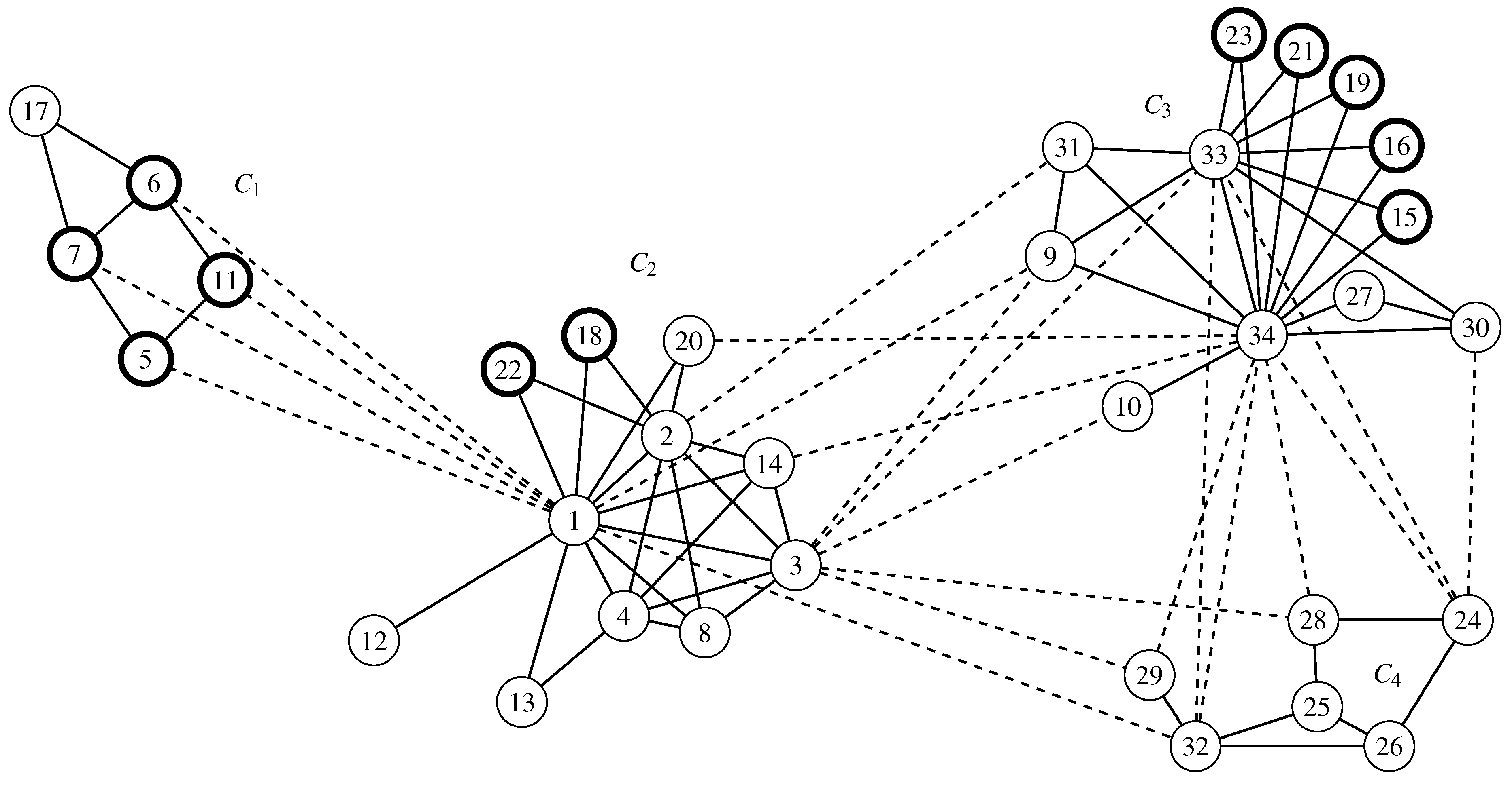
In this section, we illustrate the use of invariant measures for the three partitions ${\mathcal{P}}_O$, ${\mathcal{P}}_1$ and ${\mathcal{P}}_2$ of the Karate graph K [29], which is shown in Figure 4. $Aut\left(K\right)$ is of order 480, and it consists of the three subgroups $G_1=Sym\left({\Omega }_1\right)$ with ${\Omega }_1=\{15,16,19,21,23\}$, $G_2=Sym\left({\Omega }_2\right)$ with ${\Omega }_2=\{18,22\}$ and $G_3=\{\left(\right),\left(511\right),\left(67\right)\}$. In addition to the modularity optimal partition ${\mathcal{P}}_O$ (with its clusters separated by longer and dashed lines in Figure 4), we use the partitions ${\mathcal{P}}_1$ and ${\mathcal{P}}_2$:

$$\begin{array}{cc}\hfill {\mathcal{P}}_1=& \left\{\left\{\mathit{5},6,7,\mathbf{19},\mathbf{21}\right\},\left\{1,2,3,4,8,12,13,14,18,20,22\right\},\right.\hfill \\ & \left.\left\{9,10,\mathit{11},\mathbf{15},\mathbf{16},17,\mathbf{23},27,30,31,33,34\right\},\left\{24,25,26,28,29,32\right\}\right\}\hfill \\ \hfill {\mathcal{P}}_2=& \left\{\left\{\mathit{5},6,7,8,12,\mathbf{19},\mathbf{21}\right\},\left\{1,2,3,4,13,14,18,20,22\right\},\right.\hfill \\ & \left.\left\{9,10,\mathit{11},\mathbf{15},\mathbf{16},17,\mathbf{23},27,30,31,33,34\right\},\left\{24,25,26,28,29,32\right\}\right\}\hfill \end{array}$$

Both partitions are affected by the orbits $\{\mathbf{15},\mathbf{16},\mathbf{19},\mathbf{21},\mathbf{23}\}$ and $\{\mathit{5},\mathit{11}\}$, each overlapping two clusters. The dissimilarity to ${\mathcal{P}}_O$ is larger for ${\mathcal{P}}_2$, which is reflected in

Table 6. Diameter (computed using $d_{RI}$), orbit size and stability of partitions ${\mathcal{P}}_O$, ${\mathcal{P}}_1$ and ${\mathcal{P}}_2$.

$\mathcal{X}$	${\mathcal{P}}_{\mathit{O}}$	${\mathcal{P}}_1$	${\mathcal{P}}_2$
$dia\left(\mathcal{X}\right)$	$0.0000$	$0.1176$	$0.1390$
$|{\mathcal{X}}^{Aut\left(G\right)}|$	1	20	20
$\mathcal{X}$ stable?	yes	no	no

and

Table 7. Invariant measures and automorphism effects for the Karate graph. The R package partitionComparison has been used for the computations [23].

Measure $\mathit{d}={\mathit{d}}_{\mathit{RI}}$	$\mathit{m}({\mathcal{P}}_{\mathit{O}},{\mathcal{P}}_1)$	$\mathit{m}({\mathcal{P}}_{\mathit{O}},{\mathcal{P}}_2)$	$\mathit{m}({\mathcal{P}}_1,{\mathcal{P}}_2)$
d	$0.0927$	$0.1426$	$0.0499$
$d_L^{\ast }+d_{Aut\left(G\right)}$	$0.0927$	$0.1426$	$0.0499+0.0000$
$d_U^{\ast }-d_{Aut\left(G\right)}$	$0.0927$	$0.1426$	$0.1676-0.1176$
$d_{av}^{\ast }-d_{Aut\left(G\right)}$	$0.0927$	$0.1426$	$0.1280-0.0781$
$e_{max}^{Aut\left(K\right)}$	$0.0000$	$0.0000$	$0.1176$

.

For the optimal partition ${\mathcal{P}}_O$ of type $(5,6,11,12)$, the upper bound of the size of the equivalence class is 480 [30] (p. 112). The actual size of the equivalence class of ${\mathcal{P}}_O$ is one, which means the optimal solution is not affected by $Aut\left(K\right)$. Partition ${\mathcal{P}}_1$, which is of the same type as ${\mathcal{P}}_O$, also has an upper bound of 480 for its equivalence class. The actual size of the equivalence classes of both ${\mathcal{P}}_1$ and ${\mathcal{P}}_2$ is 20. Note that the actual size of the equivalence classes that drive the complexity of computing invariant measures is in our example far below the upper bound. Table 6 shows the diameters of the equivalence classes of the partitions.

Table 7 illustrates the decomposition into structural effects and automorphism effects for the three partitions of the Karate graph. We see that for the comparison of a stable partition (${\mathcal{P}}_O$) with one of the unstable partitions, the classic partition comparison measures are sufficient. However, when comparing the two unstable partitions ${\mathcal{P}}_1$ and ${\mathcal{P}}_2$, the structural effect ($0.0499$) is dominated by the maximal automorphism effect ($0.1176$). Furthermore, we note that the distribution of values over the orbit of the automorphism group is asymmetric (by looking at $d_L^{\ast }$, $d_U^{\ast }$ and $d_{av}^{\ast }$).

The analysis of the effects of the automorphism group of the Karate network showed that the automorphism group does not affect the stability of the optimal partition. However, the first results show that the situation is different for other networks like the Internet AS graph with 40,164 nodes and 85,123 edges (see Rossi et al. [31], and the data of of the graph tech-internet-as are from Rossi and Ahmed [32]): for this graph, several locally optimal solutions with a modularity value above $0.694$ exist, all of which are unstable. Further analysis of the structural properties of the solution landscape of this graph is work in progress.

7. Discussion, Conclusions and Outlook

In this contribution, we study the effects of graph automorphisms on partition comparison measures. Our main results are:

• A formal definition of partition stability, namely $\mathcal{P}$ is stable iff $|{\mathcal{P}}^{Aut\left(G\right)}|=1$.
• A proof of the non-invariance of all partition comparison measures if the automorphism group is nontrivial ($\left|Aut\right(G\left)\right|>1$).
• The construction of a pseudometric space of equivalence classes of graph partitions for three classes of invariant measures concerning finite permutation groups of graph automorphisms.
• The proof that the measures are invariant and that for these measures (after the transformation to a distance), the axioms of a metric space hold.
• The space of partitions is equipped with a metric (the original partition comparison measure) and a pseudometric (the invariant partition comparison measure).
• The decomposition of the value of a partition comparison measure into a structural part and a remainder that measures the effect of group actions.

Our definitions of invariant measures have the advantage that any existing partition comparison measure (as long as it is a distance or can be transformed into one) can still be used for the task. Moreover, the decomposition of measures restores the primary purpose of the existing comparison measures, which is to quantify structural difference. However, the construction of these measures leads directly to the classic graph isomorphism problem, whose complexity—despite considerable efforts and hopes to the contrary [33]—is still an open theoretical problem [34,35]. However, from a pragmatic point of view, today, quite efficient and practically usable algorithms exist to tackle the graph isomorphism problem [34]. In addition, for very large and sparse graphs, algorithms for finding generators of the automorphism group exist [11]. Therefore, this dependence on a computationally hard problem in general is not an actual disadvantage and allows one to implement the presented measure decomposition. The efficient implementation of algorithms for the decomposition of graph partition comparison measures is left for further research.

Another constraint is that we have investigated the effects of automorphisms on partition comparison measures in the setting of graph clustering only. The reason for this restriction is that the automorphism group of the graph is already defined by the graph itself and, therefore, is completely contained in the graph data. For arbitrary datasets, the information about the automorphism group is usually not contained in the data, but must be inferred from background theories. However, provided we know the automorphism group, our results on the decomposition of the measures generalize to arbitrary cluster problems.

All in all, this means that this article provides two major assets: first, it provides a theoretic framework that is independent of the preferred measure and the data. Second, we provide insights into a source of possible partition instability that has not yet been discussed in the literature. The downsides (symmetry group must be known and graph clustering only) are in our opinion not too severe, as we discussed above. Therefore, we think that our study indicates that a better understanding of the principle of symmetry is important for future research in data analysis.

References

- Melnykov, V.; Maitra, R. CARP: Software for fishing out good clustering algorithms. J. Mach. Learn. Res. 2011, 12, 69–73. [Google Scholar]
- Bader, D.A.; Meyerhenke, H.; Sanders, P.; Wagner, D. (Eds.) 10th DIMACS Implementation Challenge—Graph Partitioning and Graph Clustering; Rutgers University, DIMACS (Center for Discrete Mathematics and Theoretical Computer Science): Piscataway, NJ, USA, 2012. [Google Scholar]
- Jaccard, P. Nouvelles recherches sur la distribution florale. Bull. Soc. Vaud. Sci. Nat. 1908, 44, 223–270. [Google Scholar]
- Horta, D.; Campello, R.J.G.B. Comparing hard and overlapping clusterings. J. Mach. Learn. Res. 2015, 16, 2949–2997. [Google Scholar]
- Romano, S.; Vinh, N.X.; Bailey, J.; Verspoor, K. Adjusting for chance clustering comparison measures. J. Mach. Learn. Res. 2016, 17, 1–32. [Google Scholar]
- Von Luxburg, U.; Williamson, R.C.; Guyon, I. Clustering: Science or art? JMLR Workshop Conf. Proc. 2011, 27, 65–79. [Google Scholar]
- Hennig, C. What are the true clusters? Pattern Recognit. Lett. 2015, 64, 53–62. [Google Scholar] [CrossRef]
- Van Craenendonck, T.; Blockeel, H. Using Internal Validity Measures to Compare Clustering Algorithms; Benelearn 2015 Poster Presentations (Online); Benelearn: Delft, The Netherlands, 2015; pp. 1–8. [Google Scholar]
- Filchenkov, A.; Muravyov, S.; Parfenov, V. Towards cluster validity index evaluation and selection. In Proceedings of the 2016 IEEE Artificial Intelligence and Natural Language Conference, St. Petersburg, Russia, 10–12 November 2016; pp. 1–8. [Google Scholar]
- MacArthur, B.D.; Sánchez-García, R.J.; Anderson, J.W. Symmetry in complex networks. Discret. Appl. Math. 2008, 156, 3525–3531. [Google Scholar] [CrossRef] [Green Version]
- Darga, P.T.; Sakallah, K.A.; Markov, I.L. Faster Symmetry Discovery Using Sparsity of Symmetries. In Proceedings of the 2008 45th ACM/IEEE Design Automation Conference, Anaheim, CA, USA, 8–13 June 2008; pp. 149–154. [Google Scholar]
- Katebi, H.; Sakallah, K.A.; Markov, I.L. Graph Symmetry Detection and Canonical Labeling: Differences and Synergies. In Turing-100. The Alan Turing Centenary; EPiC Series in Computing; Voronkov, A., Ed.; EasyChair: Manchester, UK, 2012; Volume 10, pp. 181–195. [Google Scholar]
- Ball, F.; Geyer-Schulz, A. How symmetric are real-world graphs? A large-scale study. Symmetry 2018, 10, 29. [Google Scholar] [CrossRef]
- Newman, M.E.J.; Girvan, M. Finding and evaluating community structure in networks. Phys. Rev. E 2004, 69, 026113. [Google Scholar] [CrossRef] [PubMed]
- Ovelgönne, M.; Geyer-Schulz, A. An Ensemble Learning Strategy for Graph Clustering. In Graph Partitioning and Graph Clustering; Bader, D.A., Meyerhenke, H., Sanders, P., Wagner, D., Eds.; American Mathematical Society: Providence, RI, USA, 2013; Volume 588, pp. 187–205. [Google Scholar]
- Wielandt, H. Finite Permutation Groups; Academic Press: New York, NY, USA, 1964. [Google Scholar]
- James, G.; Kerber, A. The Representation Theory of the Symmetric Group. In Encyclopedia of Mathematics and Its Applications; Addison-Wesley: Reading, MA, USA, 1981; Volume 16. [Google Scholar]
- Coxeter, H.; Moser, W. Generators and Relations for Discrete Groups. In Ergebnisse der Mathematik und ihrer Grenzgebiete; Springer: Berlin, Germany, 1965; Volume 14. [Google Scholar]
- Dixon, J.D.; Mortimer, B. Permutation Groups. In Graduate Texts in Mathematics; Springer: New York, NY, USA, 1996; Volume 163. [Google Scholar]
- Beth, T.; Jungnickel, D.; Lenz, H. Design Theory; Cambridge University Press: Cambridge, UK, 1993. [Google Scholar]
- Erdős, P.; Rényi, A.; Sós, V.T. On a problem of graph theory. Stud. Sci. Math. Hung. 1966, 1, 215–235. [Google Scholar]
- Burr, S.A.; Erdős, P.; Spencer, J.H. Ramsey theorems for multiple copies of graphs. Trans. Am. Math. Soc. 1975, 209, 87–99. [Google Scholar] [CrossRef]
- Ball, F.; Geyer-Schulz, A. R Package Partition Comparison; Technical Report 1-2017, Information Services and Electronic Markets, Institute of Information Systems and Marketing; KIT: Karlsruhe, Germany, 2017. [Google Scholar]
- Doob, J.L. Measure Theory. In Graduate Texts in Mathematics; Springer: New York, NY, USA, 1994. [Google Scholar]
- Hausdorff, F. Set Theory, 2nd ed.; Chelsea Publishing Company: New York, NY, USA, 1962. [Google Scholar]
- Kuratowski, K. Topology Volume I; Academic Press: New York, NY, USA, 1966; Volume 1. [Google Scholar]
- Von Neumann, J. Construction of Haar’s invariant measure in groups by approximately equidistributed finite point sets and explicit evaluations of approximations. In Invariant Measures; American Mathematical Society: Providence, RI, USA, 1999; Chapter 6; pp. 87–134. [Google Scholar]
- Ball, F.; Geyer-Schulz, A. Weak invariants of actions of the automorphism group of a graph. Arch. Data Sci. Ser. A 2017, 2, 1–22. [Google Scholar]
- Zachary, W.W. An information flow model for conflict and fission in small groups. J. Anthropol. Res. 1977, 33, 452–473. [Google Scholar] [CrossRef]
- Bock, H.H. Automatische Klassifikation: Theoretische und praktische Methoden zur Gruppierung und Strukturierung von Daten; Vandenhoeck und Ruprecht: Göttingen, Germany, 1974. [Google Scholar]
- Rossi, R.; Fahmy, S.; Talukder, N. A Multi-level Approach for Evaluating Internet Topology Generators. In Proceedings of the 2013 IFIP Networking Conference, Trondheim, Norway, 2–4 June 2013; pp. 1–9. [Google Scholar]
- Rossi, R.A.; Ahmed, N.K. The Network Data Repository with Interactive Graph Analytics and Visualization. In Proceedings of the Twenty-Ninth AAAI Conference on Artificial Intelligence, Austin, TX, USA, 25–30 January 2015. [Google Scholar]
- Furst, M.; Hopcroft, J.; Luks, E. Polynomial-time Algorithms for Permutation Groups. In Proceedings of the 21st Annual Symposium on Foundations of Computer Science, Syracuse, NY, USA, 13–15 October 1980; pp. 36–41. [Google Scholar]
- McKay, B.D.; Piperno, A. Practical graph isomorphism, II. J. Symb. Comput. 2014, 60, 94–112. [Google Scholar] [CrossRef] [Green Version]
- Babai, L. Graph isomorphism in quasipolynomial time. arXiv, 2015; arXiv:1512.03547. [Google Scholar]
- Fortunato, S.; Barthélemy, M. Resolution limit in community detection. Proc. Natl. Acad. Sci. USA 2007, 104, 36–41. [Google Scholar] [CrossRef] [PubMed]
- Lancichinetti, A.; Fortunato, S. Limits of modularity maximization in community detection. Phys. Rev. E 2011, 84, 66122. [Google Scholar] [CrossRef] [PubMed]
- Geyer-Schulz, A.; Ovelgönne, M.; Stein, M. Modified randomized modularity clustering: Adapting the resolution limit. In Algorithms from and for Nature and Life; Lausen, B., Van den Poel, D., Ultsch, A., Eds.; Studies in Classification, Data Analysis, and Knowledge Organization; Springer International Publishing: Heidelberg, Germany, 2013; pp. 355–363. [Google Scholar]
- Meilǎ, M. Comparing clusterings—An information based distance. J. Multivar. Anal. 2007, 98, 873–895. [Google Scholar] [CrossRef]
- Youness, G.; Saporta, G. Some measures of agreement between close partitions. Student 2004, 51, 1–12. [Google Scholar]
- Denœud, L.; Guénoche, A. Comparison of distance indices between partitions. In Data Science and Classification; Batagelj, V., Bock, H.H., Ferligoj, A., Žiberna, A., Eds.; Studies in Classification, Data Analysis, and Knowledge Organization; Springer: Berlin/Heidelberg, Germany, 2006; pp. 21–28. [Google Scholar]
- Albatineh, A.N.; Niewiadomska-Bugaj, M.; Mihalko, D. On similarity indices and correction for chance agreement. J. Classif. 2006, 23, 301–313. [Google Scholar] [CrossRef]
- Rand, W.M. Objective criteria for the evaluation of clustering algorithms. J. Am. Stat. Assoc. 1971, 66, 846–850. [Google Scholar] [CrossRef]
- Hubert, L.; Arabie, P. Comparing partitions. J. Classif. 1985, 2, 193–218. [Google Scholar] [CrossRef]
- Hamann, U. Merkmalsbestand und Verwandtschaftsbeziehungen der Farinosae: Ein Beitrag zum System der Monokotyledonen. Willdenowia 1961, 2, 639–768. [Google Scholar]
- Czekanowski, J. “Coefficient of Racial Likeness” und “Durchschnittliche Differenz”. Anthropol. Anz. 1932, 9, 227–249. [Google Scholar]
- Kulczynski, S. Zespoly roslin w Pieninach. Bull. Int. Acad. Pol. Sci. Lett. 1927, 2, 57–203. [Google Scholar]
- McConnaughey, B.H. The determination and analysis of plankton communities. Mar. Res. 1964, 1, 1–40. [Google Scholar]
- Peirce, C.S. The numerical measure of the success of predictions. Science 1884, 4, 453–454. [Google Scholar] [CrossRef] [PubMed]
- Wallace, D.L. A method for comparing two hierarchical clusterings: Comment. J. Am. Stat. Assoc. 1983, 78, 569–576. [Google Scholar] [CrossRef]
- Fowlkes, E.B.; Mallows, C.L. A method for comparing two hierarchical clusterings. J. Am. Stat. Assoc. 1983, 78, 553–569. [Google Scholar] [CrossRef]
- Yule, G.U. On the association of attributes in statistics: With illustrations from the material of the childhood society. Philos. Trans. R. Soc. A 1900, 194, 257–319. [Google Scholar] [CrossRef]
- Sokal, R.R.; Sneath, P.H.A. Principles of Numerical Taxonomy; W. H. Freeman: San Francisco, CA, USA; London, UK, 1963. [Google Scholar]
- Baulieu, F.B. A classification of presence/absence based dissimilarity coefficients. J. Classif. 1989, 6, 233–246. [Google Scholar] [CrossRef]
- Gower, J.C.; Legendre, P. Metric and euclidean properties of dissimilarity coefficients. J. Classif. 1986, 3, 5–48. [Google Scholar] [CrossRef]
- Rogers, D.J.; Tanimoto, T.T. A computer program for classifying plants. Science 1960, 132, 1115–1118. [Google Scholar] [CrossRef] [PubMed]
- Goodman, L.A.; Kruskal, W.H. Measures of association for cross classifications. J. Am. Stat. Assoc. 1954, 49, 732–764. [Google Scholar]
- Robert, P.; Escoufier, Y. A unifying tool for linear multivariate statistical methods: The RV-coefficient. J. R. Stat. Soc. Ser. C 1976, 25, 257–265. [Google Scholar] [CrossRef]
- Russel, P.F.; Rao, T.R. On habitat and association of species of anopheline larvae in south-eastern madras. J. Malar. Inst. India 1940, 3, 153–178. [Google Scholar]
- Mirkin, B.G.; Chernyi, L.B. Measurement of the distance between partitions of a finite set of objects. Autom. Remote Control 1970, 31, 786–792. [Google Scholar]
- Hilbert, D. Gesammelte Abhandlungen von Hermann Minkowski, Zweiter Band; Number 2; B. G. Teubner: Leipzig, UK; Berlin, Germany, 1911. [Google Scholar]
- Pearson, K. On the coefficient of racial likeness. Biometrika 1926, 18, 105–117. [Google Scholar] [CrossRef]
- Lerman, I.C. Comparing Partitions (Mathematical and Statistical Aspects). In Classification and Related Methods of Data Analysis; Bock, H.H., Ed.; North-Holland: Amsterdam, The Netherlands, 1988; pp. 121–132. [Google Scholar]
- Fager, E.W.; McGowan, J.A. Zooplankton species groups in the north pacific co-occurrences of species can be used to derive groups whose members react similarly to water-mass types. Science 1963, 140, 453–460. [Google Scholar] [CrossRef] [PubMed]
- Larsen, B.; Aone, C. Fast and Effective Text Mining Using Linear-time Document Clustering. In Proceedings of the Fifth ACM SIGKDD International Conference on Knowledge Discovery and Data Mining, San Diego, CA, USA, 15–18 August 1999; ACM: New York, NY, USA, 1999; pp. 16–22. [Google Scholar]
- Meilǎ, M.; Heckerman, D. An experimental comparison of model-based clustering methods. Mach. Learn. 2001, 42, 9–29. [Google Scholar] [CrossRef]
- Van Dongen, S. Performance Criteria for Graph Clustering and Markov Cluster Experiments; Technical Report INS-R 0012; CWI (Centre for Mathematics and Computer Science): Amsterdam, The Netherlands, 2000. [Google Scholar]
- Vinh, N.X.; Epps, J.; Bailey, J. Information theoretic measures for clusterings comparison: Variants, properties, normalization and correction for chance. J. Mach. Learn. Res. 2010, 11, 2837–2854. [Google Scholar]
- Meilǎ, M. Comparing clusterings by the variation of information. In Learning Theory and Kernel Machines; Schölkopf, B., Warmuth, M.K., Eds.; Number 2777 in Lecture Notes in Computer Science; Springer: Berlin/Heidelberg, Germany, 2003; pp. 173–187. [Google Scholar]
- Danon, L.; Díaz-Guilera, A.; Duch, J.; Arenas, A. Comparing community structure identification. J. Stat. Mech. Theory Exp. 2005, 2005, P09008. [Google Scholar] [CrossRef]
Figure 1.
Two structurally different partitions of the cycle graph C4: grouping pairs of neighbors (a) and grouping pairs of diagonals (d). Equally-colored nodes represent graph clusters, and the choice of colors is arbitrary. Adding, again arbitrary, but fixed, node labels impacts the node partitions and results in the failure to recognize the structural difference when comparing these partitions with partition comparison measures (see Table 1). The different images (b,c) (, and (e,f) ) emerge from the graph’s symmetry.
Figure 2.
The butterfly graph (five nodes, with two node pairs connected by the bridging node 3).
Figure 3.
The cycle graph (the “outer” cycle) and an initial partition of six clusters (connected nodes of the same color, separated by dashed lines). A single application of “rotates” the graph by one node (the “inner” cycle ). As a consequence, in each cluster, one node drops out and is added to another cluster: For instance, Node 1 drops out of the “original” cluster , and Node 7 is added, resulting in . All dropped nodes are shown in light gray.
Figure 4.
Zachary’s Karate graph K with the vertices of the orbits of the three subgroups of in bold and the clusters of separated by dashed edges.