Application of Relative Entropy and Gradient Boosting Decision Tree to Fault Prognosis in Electronic Circuits


1
Department of Communication, National Digital Switching System Engineering and Technology R&D Center(NDSC), Zhengzhou 450002, China
2
College of Mechanical and Electrical Engineering, Henan Agricultural University, Zhengzhou 450002, China
*
Author to whom correspondence should be addressed.
Symmetry 2018, 10(10), 495; https://doi.org/10.3390/sym10100495
Submission received: 25 September 2018
/
Revised: 11 October 2018
/
Accepted: 11 October 2018
/
Published: 15 October 2018
Abstract
:Fault prognosis of electronic circuits is the premise of guaranteeing normal operation of a system and carrying out on-condition maintenance. In this work, the remaining useful life (RUL) of electronic elements was estimated by selecting fault features based on variance, measuring fault severity based on relative entropy distance, and conducting fault prognosis based on the gradient boosting decision tree (GBDT) model. At first, the corresponding voltages of amplitude-frequency response, under conditions of changing full-band element parameters, were extracted, and then the frequency bands with large change amplitude were further selected based on variance. Afterwards, using relative entropy distance, the degradation of element parameters was measured, and then the RUL of electronic elements was diagnosed through regression analysis by GBDT. By comparing the data with those arising from the use of other distance-measuring methods, the relative entropy distance shows a larger change range and less apt to suffer interference from noise, which is favorable to subsequent regression prediction. The regression analysis through GBDT is easy to understand and conveniently applied in engineering practice. The application of the method proposed in the study in two examples of electronic circuits indicates that the prediction accuracy of the method for RUL of electronic elements is higher than that of the other distance-measuring methods, and its application in engineering practice is convenient.
1. Introduction
Prognostic and health management (PHM) is a health management programme used to observe the operational state of equipment proposed by comprehensively utilizing the latest research achievements of modern information and artificial intelligence technologies. A PHM system can predict the possibility of system failure in a given period of time in the future and guide measures for on-condition maintenance. In electronic systems, PHM needs to foresee the elements probably being subjected to faults and evaluate the remaining useful life (RUL) of systems in advance, realizing the on-condition maintenance of electronic systems [1,2,3,4]. Because of the processing technique and working mechanism, the electronic elements of an electronic system are inevitably subjected to degradation-induced faults, such as aging and parameter drift. The high temperatures induced by long-term operation can also accelerate the aging rate until the elements lose their efficacy. The premise for conducing fault prognosis of electronic elements is to extract effective fault features. According to distance of fault features to the state of normal elements, the health of an element could be measured. That is, the degree of deviation of a given fault state from the norm needs to be quantified using a fault indicator (FI).
The easily measured voltages of some circuits are generally taken as extracted features. For example, in the literature [5,6,7,8,9,10,11], the voltage signals in the amplitude-frequency response curve were uniformly extracted as eigenvalues. Owing to the large dataset, the voltage amplitudes of frequency response corresponding to typical frequencies were selected as eigenvalues [7,12,13]. In the literature [5], the first five voltage features output from amplitude-frequency characteristic curves were preferentially selected based on a minimum redundancy maximum relevance (mRMR) principle and were considered as the optimal fault features.
The health of an element is generally measured on the basis of distance. For example, in the literature [6,12,13], the degradation of elements was measured using cosine distance and Pearson’s correlation coefficient and calculated by extracting signals containing the frequency-domain response of circuits under test to characterise the health of circuit elements. The change range of cosine distance and Pearson’s correlation coefficient in literature is [1 0.996], in the literature [10], Euclidean distance was applied as the FI. In the literature [8,9,10], the eigenvalues were extracted by applying a wavelet packet transform and the health of elements was measured based on Pearson’s correlation coefficient and Euclidean distance. Afterwards, the RUL of electronic elements was predicted by carrying out regression analyses using support vector machines [5,6,7,8,9,10,11,12,13] and particle filters [14] based on FI. Gradient boosting decision tree (GBDT) can be applied to both regression and classification, with the advantages of completeness, robustness, and a good explanation therewith. It has been used in the virtual screening for hyperuricemia [15], soil property retrieval [16], and short-term subway ridership [17]; however, it has not yet been applied in fault prognosis.
The rate of change in the health of elements calculated after extracting features based on the methods is extremely small, resulting in poor anti-jamming ability and a finite prediction accuracy for RUL. To improve the prediction accuracy for RUL of elements, the characteristic quantity of elements with a large variance in their degradation was extracted using variance selection. Compared with existing methods in which features are not screened, or are selected according to experience, the method can be applied to select several features that make greatest contributions to component health and RUL of elements to simplify the subsequent computations. Compared with the other measurement methods, the method of measuring the health of elements using relative entropy distance shows greater amplitude of change, which is favorable for subsequent prediction for RUL. The RUL prediction was carried out using regression analysis based on ensemble learning, that is, multiple weak classifier models were integrated to form a strong classifier to solve over-fitting issues, enhance the generalization performance of models, and thus improve the accuracy of prediction.
The rest of the study is presented as follows. Section 2 explains how to acquire the degradation features of elements and define their health, Section 3 covers the method for fault diagnosis based on a gradient boosting decision tree (GBDT), Section 4 presents the simulation process and predicted result, and conclusions are drawn in Section 5.
2. Processing of Fault Data
By analyzing the operational process of an analogue circuit, it can be seen that (1) the circuit is in a healthy state over the long-term and thus plenty of healthy samples can be obtained; (2) the features in a fault state are significantly different from those in a healthy state so that fault information is easily distinguished from healthy information, for example, the voltage in fault state is lower than the healthy state. That is, faults are easily found from the circuit features; however, it is difficult to evaluate the degree of parameter degradation induced by a fault among various elements. Therefore, how to define the health of elements according to a feature set is critical. The parameter degradation-induced faults of resistors and capacitors in an analogue circuit greatly influence the performance of the circuit as explored here.
2.1. Feature Extraction
While extracting engineering features from time-domain response signals, time series are vulnerable to noise, likely to be scaling or shifting [18]. The frequency-domain analysis of analog circuits can provide feature information that is more intuitive than time-domain waveform data. Therefore, the voltage value on the frequency-response curve is selected as the eigenvector. Owing to the change of electronic elements generally influencing the specific frequency bands of the frequency response instead of the full-wave band, the voltage corresponding to the frequency band with the greatest change in output voltage is taken as the eigenvector. By employing a variance-based selection method, features are selected to extract the features showing the most change. The specific process is as follows: variances of various features are calculated and then based on the threshold value; the features whose variance exceeds the threshold value are selected.
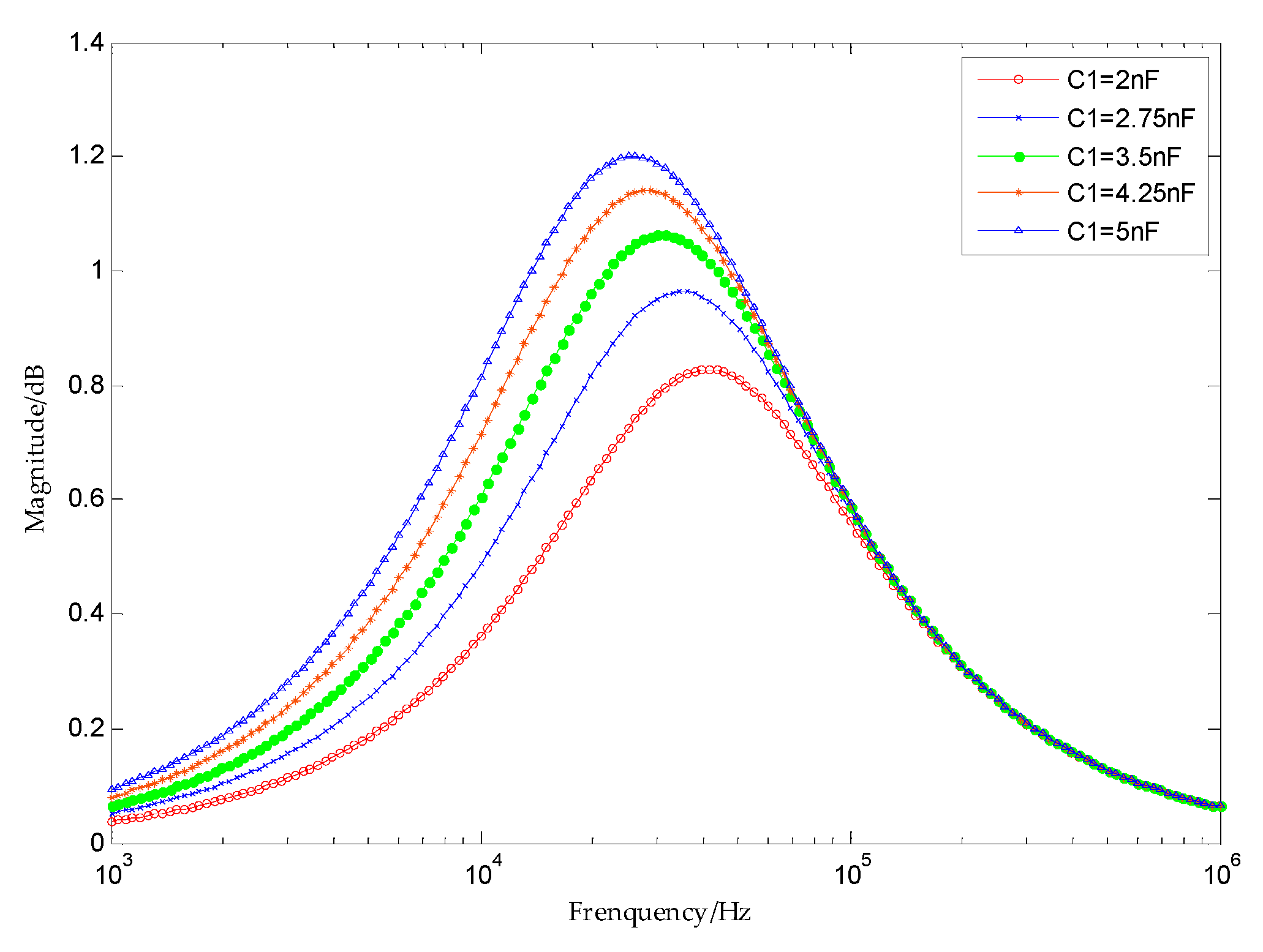
Figure 1 shows the frequency-response curve of a representative element during the degradation of parameters, from the amplitude-frequency characteristic curve of the circuit, it can be seen that the influence of the change in C1 on the circuit is mainly concentrated in the low-frequency band, but exhibits almost no change in the high-frequency band. Therefore, it is feasible to extract the voltage features corresponding to the first n frequency bands by utilizing variance selection, while ignoring the voltage values in redundant frequency bands with an insignificant change of variance.
2.2. FI
The relative entropy is also called Kullback–Leible divergence (namely, KL divergence), [19,20,21,22]. It is supposed that and are two probability distributions of , so the relative entropy between and can be expressed as follows:
To some extent, entropy can measure the distance between two random variables. The relative entropy is an asymmetric measurement of the two probability distributions and . When the random distributions of the two variables are same, the relative entropy between the two variables is zero. On the condition that the random distributions of the two variables show a significant difference, the relative entropy between the two variables increases [22,23].
In terms of the definition of FI, the parameter degradation-induced faults and normal work of electronic elements are seen as two random states of the electronic element x. The voltage during a degradation-induced fault is regarded as the probability distribution of the output value in a true state, while the output voltage value in a normal state is taken as the theoretical probability distribution . Moreover, the relative entropy between degradation-induced fault and normal work is considered as the FI. When the element works normally, the relative entropy between the two conditions is zero. As the severity of the degradation-induced fault of the element increases, the relative entropy increases.
3. GBDT
GBDT, the gradient boosted decision tree or gradient boosted regression tree, is an iteratively accumulative decision tree algorithm. The algorithm can accumulate the results of multiple decision trees as the final prediction output by establishing a group of weak learners [24,25,26]. Its minimum loss function is expressed as follows:
where , , , and refer to the input sample, classification and regression tree (CART), parameters of CART, and weights of each tree, respectively. The process of regression analysis using GBDT is as follows.
The training set sample is input, with maximum number of iterations T and loss function L. A strong learner is output.
- (1)
- Initializing weak learners
- (2)
- As for the iterations t = 1, 2, …, T, so
- (a)
- Based on the sample i = 1, 2, …, m, the negative gradient is calculated:
- (b)
- Using , a CART is fitted to acquire the tth regression tree, whose corresponding leaf node is . Here, J refers to the number of leaf nodes of the regression tree t.
- (c)
- The best-fit value is calculated according to the leaf region .
- (d)
- Updating the strong learners,
- (3)
- The expression of the strong learner f(x) is thus attained:
The important parameters of GBDT are divided into two types: important parameters of the boosting framework and the weak learner ART. Boosting a framework mainly involves the following parameters: n_estimators (the maximum number of weak learners), poor fitting easily appears under a low number of n_estimators, while over-fitting easily occurs under an extremely large number of n_estimators; learning_rate, the weight reduction coefficient (also called step length) of each weak learner. For the same fitting effect from a given training set, a low learning_rate means more iterations need to be carried out for weak learners. Generally, the fitting effect of the algorithm is determined according to the step length and the maximum number of iterations; therefore, the two parameters (n_estimators and learning_rate) need to be synchronously adjusted; if the value of a sub-sample of the data is 1, all of the samples are applied, which indicates that sub-sampling is not used. If the value is smaller than 1, only some of samples are applied for the fitting of GBDT. Selecting the ratio lower than 1 can reduce variance, that is, preventing over-fitting; however, it can increase the deviation of sample fitting and therefore the value of sub-sample should not be too low. Loss refers to the loss function of the algorithm, and the mean square error (MSE) “ls” loss function is applied for the regression model. The prediction error is evaluated using the root mean square error (RMSE) between the predicted and actual values, which is the square root of the ratio of the square of the deviation between observed and actual values after n observations. The RMSE can reflect the goodness of fit between predicted and true values:
where and denote the predicted and actual values of the ith iteration, respectively.
In practical working environments, interference is inevitable; as common noise sources (thermal noise and shot noise) are Gaussian white noise and are generally taken as the ideal model of additive noise. The power spectrum of the noise is uniformly distributed, while its amplitude conforms to a Gaussian distribution. Moreover, two random variables at any two times are irrelevant and show statistical independence. The fault measurement of the measured electronic element is simulated by adding Gaussian white noise on the distance of relative entropy.
The parameter adjustment based on GBDT is performed using grid search and the sub-sample is generally in the range of 0.5 to 0.8 to improve operational efficiency. At first, a large step length (learning_rate) and low iterative times (n_estimators) are selected. The grid search is conducted by setting the step length (learning_rate) as 0.1 and the number of iterations (n_estimators) in the range of 10 to 100. After determining the iterative times, the step length is optimized.
4. Example Analysis
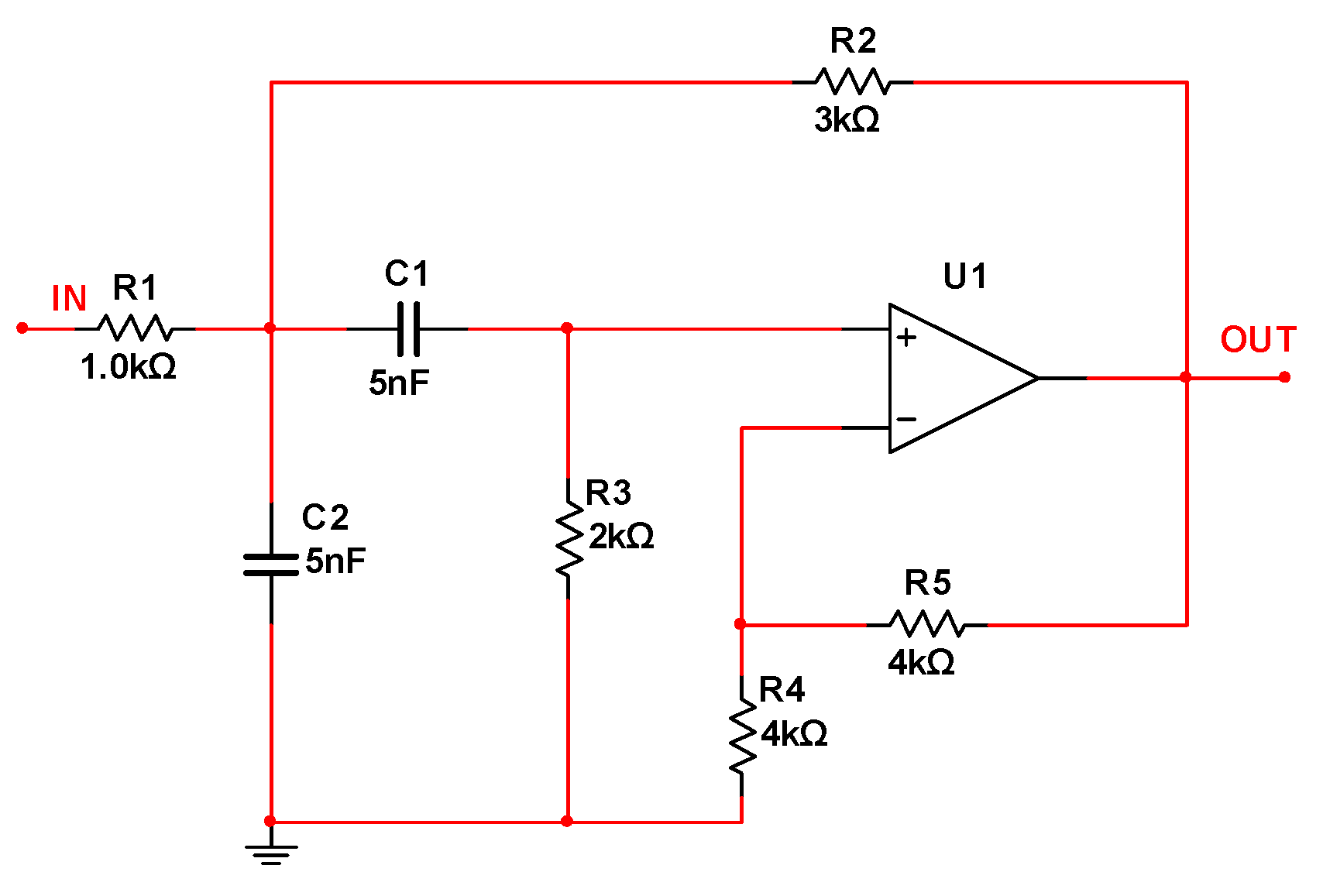
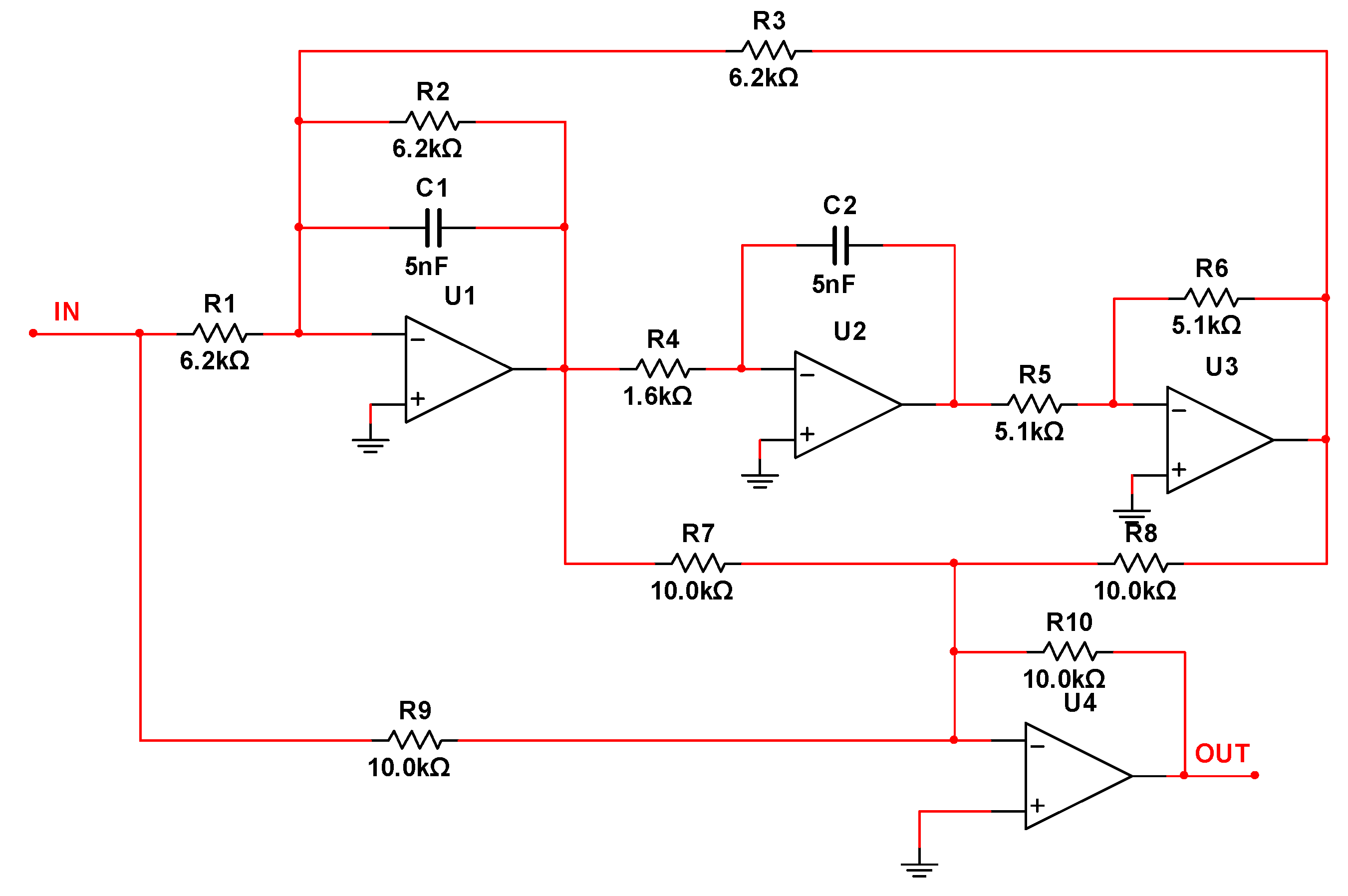
The Sallen–key filter and Tow–Thomas filter circuits are commonly used for fault diagnosis and fault prognosis of analogue circuits. To compare with current research results, the two circuits were also applied in the present study. Figure 2 shows the schematic diagram of a Sallen–key filter circuit, while Figure 3 illustrates that of the Tow–Thomas filter circuit. By selecting and analyzing the individual elements in each circuit most influencing the output, it can be seen that it is crucial to the performance of the whole circuit to predict the RULs of the elements therein.
In these circuits, degradation-induced faults in both capacitors and resistors were analyzed. The reason for this is that the capacitor is prone to electric charge leakage. When the electric leakage happens, the insulating property between the two polar plates of the capacitor decreases and thus leakage resistance appears between them. In this way, direct-current (DC) current passes through the capacitor. The blocking performance of the capacitor is reduced and its charge capacity decreases. This is a common fault in small capacitors and is hard to detect. The parameter degradation-induced faults of different resistance manufacturing technologies show diverse manifestations, while a majority of degradation-induced faults of resistors are seen as upward resistance drift. Therefore, the literature [12,13,27] shows evidence of such parameter degradation-induced faults in which resistance increases while capacitance decreases. In reference to each time index in the literature [27,28], the resistance and capacitance both vary at a rate of 0.4%. When a parameter of an electronic element deviates by 50% from its nominal value, it is inferred that a fault occurs [27,28]. Within the parameter degradation range of 60%, the analysis and RUL prediction were carried out, therefore, the output changes of each element were analyzed under 150 time indices and the 125th time index was taken as the fault threshold. Each of the two circuits was separately analyzed in the following sections.
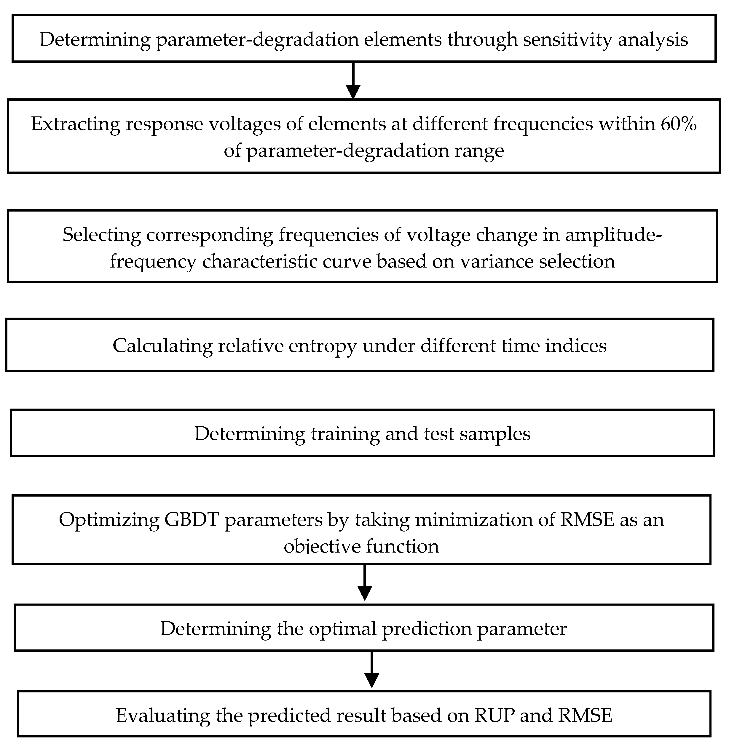
The specific process of fault prediction is shown in Figure 4.
The specific process is described as follows:
- (1)
- There are numerous electronic elements in circuit systems. The elements prone to faults are determined according to sensitivity analysis and expert experience. A hard fault is the most extreme form of parameter degradation-induced faults, and is caused by the deterioration of parameter degradation-induced faults. Therefore, predicting parameter degradation-induced faults in electronic elements is key to conducting on-condition maintenance of circuit systems.
- (2)
- The common parameter degradation-induced faults in which capacitance gradually decreases, while resistance gradually increases, are analyzed. The characteristic curve of the amplitude-frequency response of the fault within its parameter-degradation range is extracted.
- (3)
- At different frequencies, some voltage amplitudes undergo no significant change and even remain unchanged. To improve the prediction efficiency, only those frequencies with a large amplitude change in the amplitude-frequency response curve within the parameter-degradation range were extracted for analysis.
- (4)
- By applying the relative entropy distance, the changes in output voltages of specific frequency responses under nominal values were examined with the changes in the parameters of some key electronic elements.
- (5)
- In the curve of relative entropy distance, the first 100 time indices were selected as training samples while the 101st to 150th time indices were taken as testing samples to carry out fault prediction.
- (6)
- By taking the RMSE of predicted and tested values as the objective function, the parameters of GBDT were optimized to determine the best predicted result.
- (7)
- Based on a predicted rational unified process (RUP) and RMSE, the prediction model was evaluated.
4.1. Feature Extraction and FI
4.1.1. The Sallen–Key Band-Pass FILTER Circuit
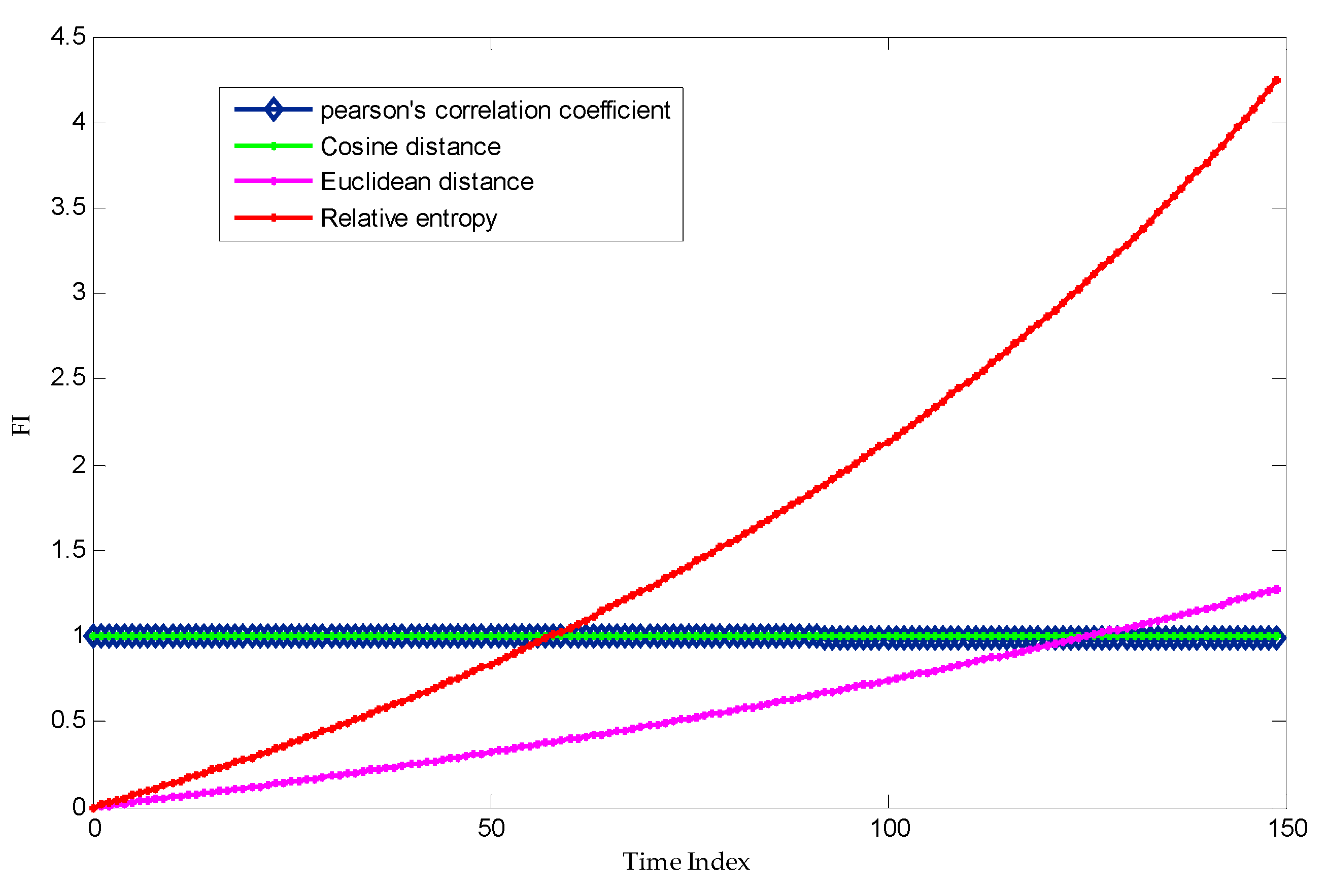
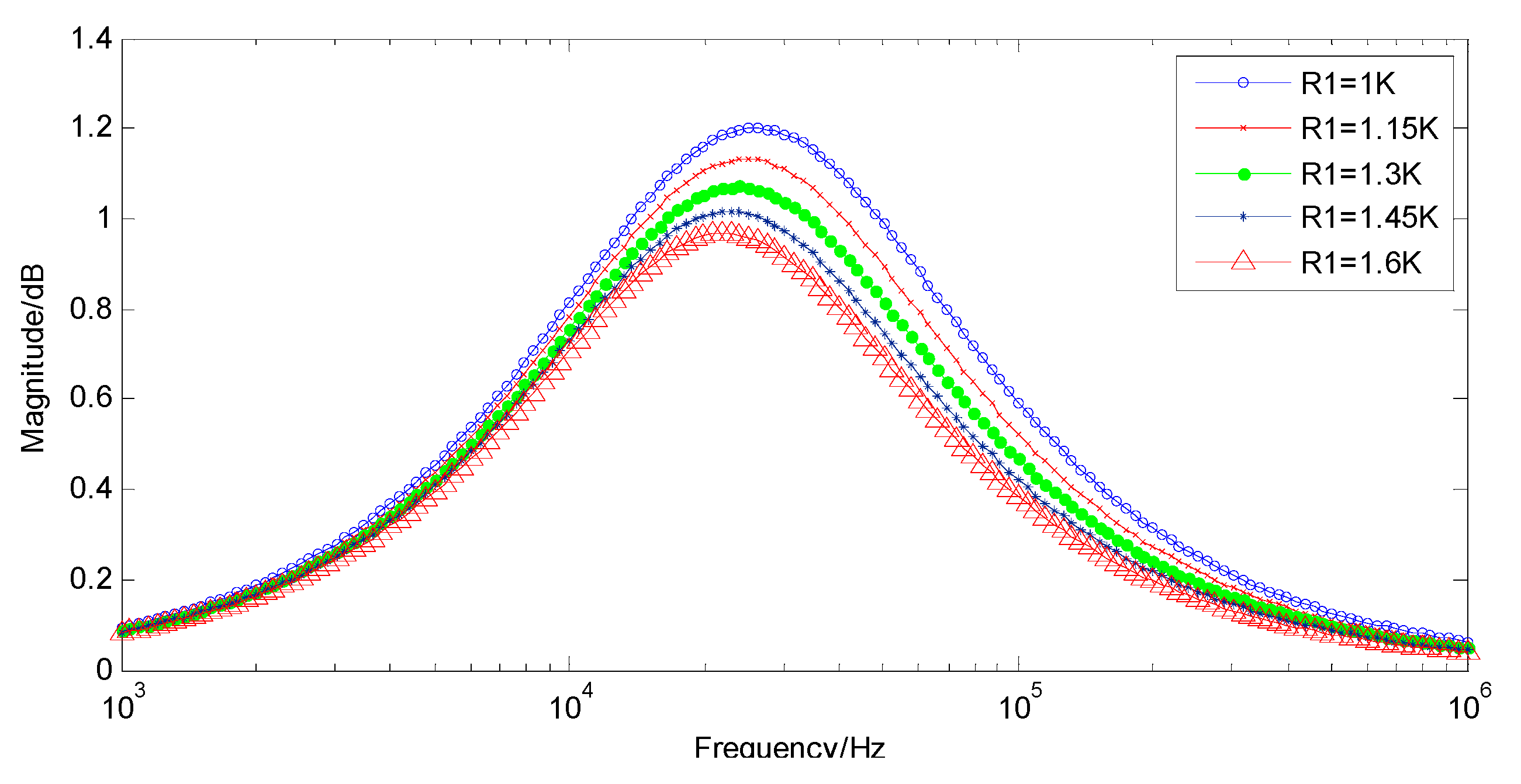
Through sensitivity analysis, it can be seen that the parameter changes of C1, C2, and R1 significantly influence the output. In terms of capacitor and resistor, C1 and R1 were taken separately as examples. According to the results of a parameter sweep, the change in C1 mainly influences the low-frequency part and does not significantly influence the high-frequency part. Figure 1 shows the spectral characteristic curve of C1 within the degradation ranges of parameters. Within the spectral response range, the characteristic voltages with variance greater than 0.02 were selected using the variance-based selection method, whose corresponding frequencies are 125,89.25 Hz, 14,125.38 Hz, 15,848.93 Hz, 17,782.79 Hz, 19,952.62 Hz, and 22,387.21 Hz, respectively. A comparison was made among the characteristic voltages in terms of the Pearson’s correlation coefficient, cosine distance, Euclidean distance, and distance of relative entropy, as shown in Figure 5. Among them, the cosine distance and Pearson’s correlation coefficient show a lower amplitude change over [1 0.996], akin to data shown in Figure 5. The result is consistent with the calculated results as in references [6,7,12,13]. It can be seen from Figure 5 that the relative entropy varies over [0 4.3] and the amplitude of the changes therein increases by about four times compared with commonly-used Euclidean distance measures in the range [0 1.1]. Hence, the former is more conducive to subsequent fault prediction; therefore, the relative entropy was applied to measure the health of elements.
When R1 increases, the amplitude-frequency scanning curve is shown in Figure 6 and the change in R1 mainly influences the amplitude of the high-frequency section. By applying the variance-selection method, the feature voltage values with a variance greater than 0.065 were selected, whose corresponding frequencies are 35,481.34 Hz, 39,810.72 Hz, 44,668.36 Hz, 50,118.72 Hz, and 56,234.13 Hz, respectively.
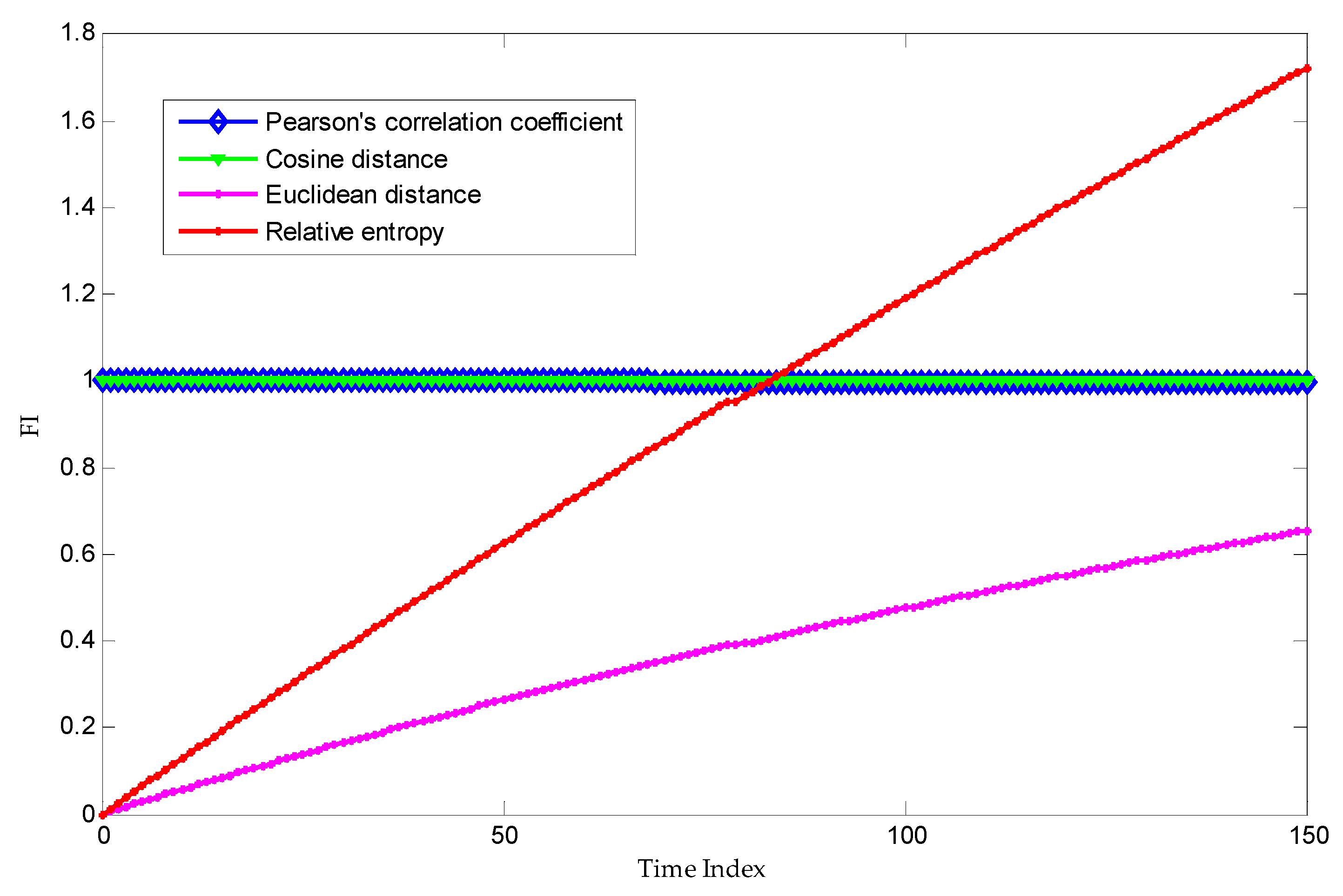
It can be seen from Figure 7 that, within the range of change of R1, the cosine distance and Pearson’s correlation coefficient change within [1 0.996] and are similar. The change in relative entropy of R1 is much greater than that in the cosine distance and Pearson’s correlation coefficient. The relative entropy changes in the range [0 1.8] and its amplitude of change increases nearly three-fold compared with the commonly-used Euclidean distance showing a range of change of [0 0.6]. Through these comparisons, it is shown that using relative entropy to measure faults deviating from normal states (FI) in the commonly used distance measurement shows a few advantages: a large amplitude change and a favorable linearity of FI. In the subsequent analysis, the FI measurement curve of relative entropy is presented.
4.1.2. The Tow–Thomas Filter Circuit
Both C2 and R4, with their high sensitivities, were selected for fault prediction and analysis of RUL of elements.
- (1)
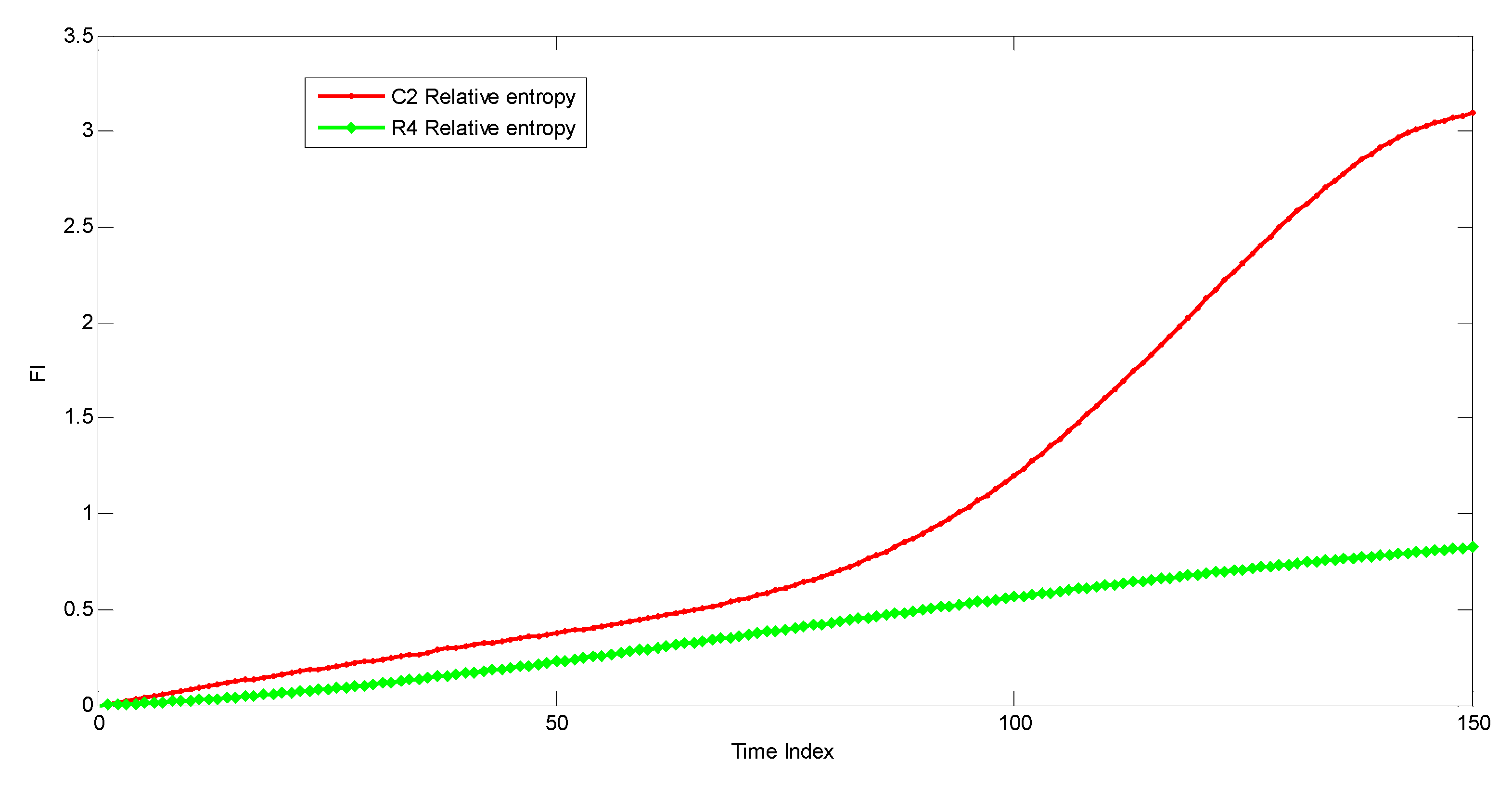
- Fault prediction for C2 was carried out using variance-based selection on its amplitude-frequency response: the voltages with a variance greater than 0.1 were selected, whose corresponding frequencies are 8912.509 Hz, 10 KHz, 11,220.18 Hz, 14,125.38 Hz, and 15,848.93 Hz, respectively. The relative entropies between the voltages values and amplitude-frequency voltage under nominal value conditions were calculated (Figure 8).
- (2)
- Fault prediction for R4 was conducted using variance-based selection on its amplitude-frequency response: the voltages with a variance greater than 0.015 were selected, whose corresponding frequencies are 6309.573 Hz, 7079.458 Hz, 7943.282 Hz, 11,220.18 Hz, and 12,589.25 Hz, respectively. The relative entropies between the voltages values and amplitude-frequency voltage under nominal value conditions were calculated (Figure 8). The changes in R4 mainly result in the forward shift of the cut-off frequency of the filter. Although the voltage changes at around 10 kHz, the relative entropy undergoes little change owing to the similar distribution of the model data.
4.2. Fault Prognostic
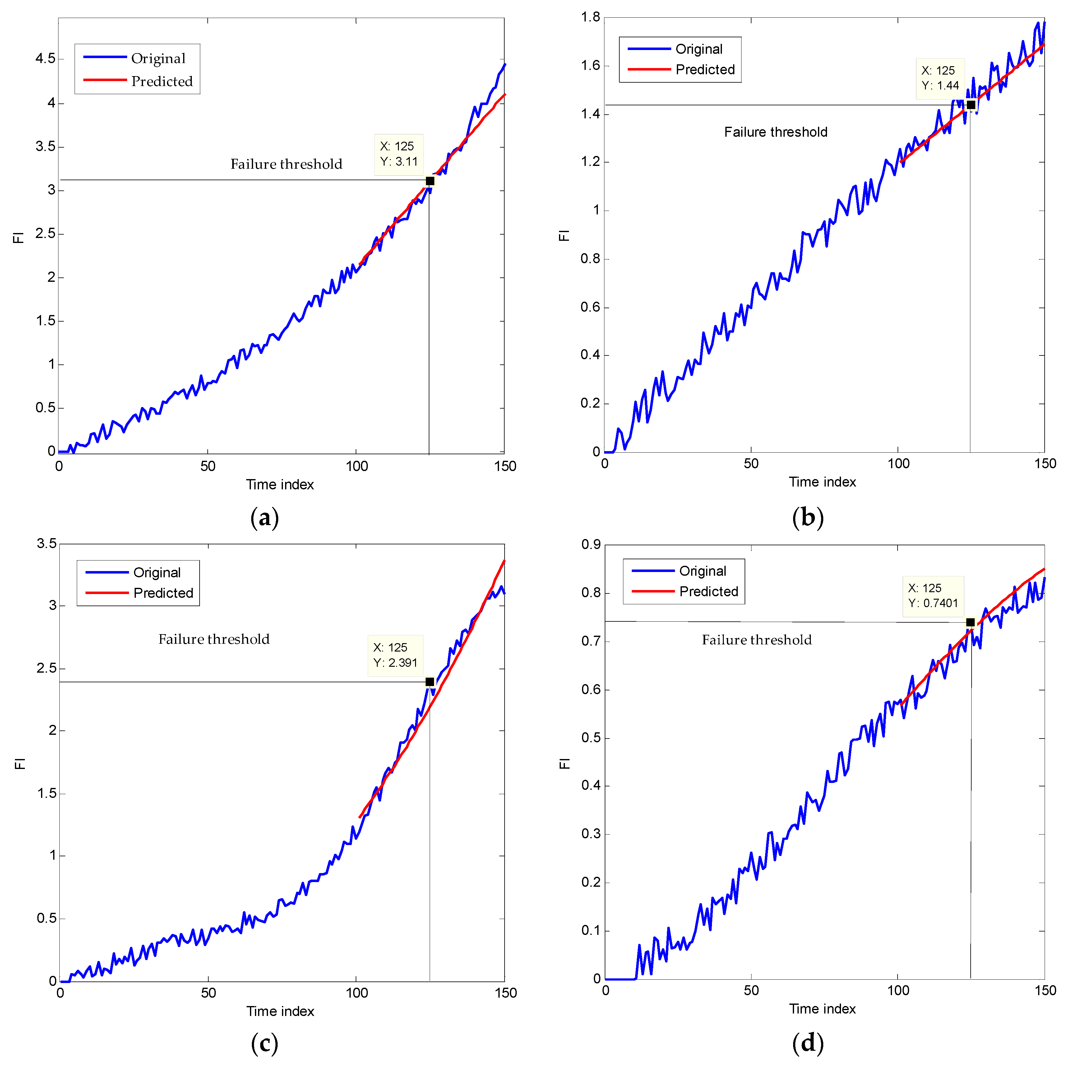
By applying Sallen–key filter and Tow–Thomas filter circuits, the method for fault prediction proposed in the study was verified. As stated above, by taking the parameter degradation of capacitor C1 and resistor R1 of Sallen–key filter circuit and the capacitor C2 and resistor R4 of a Tow–Thomas filter circuit as examples, the parameters degrade at the rate of 0.4% under each time index. When the parameter changes by 60%, there are 150 time indices. For each element, the first 100 time indices were taken as training data, while the last 50 were used for fault prediction; however, a circuit element that deviates by 50% from the nominal value is assumed faulty, that is, the 125th time index is the failure threshold of the element.
The RUL of elements is defined as follows:
where , , and represent the actual RUL of the elements, the time index corresponding to failure threshold, and the current time index, respectively.
where and refer to the predicted RUL of the elements and the time index corresponding to predicted failure threshold, respectively. The prediction error was evaluated using the 101st to 150th time indices.
The optimal parameters of GBDT of each element are listed in Table 1 and the predicted result and the curve obtained after adding Gaussian white noise, are shown in Figure 9. The predicted result shown as Table 2. The accuracy was calculated according to Formula (11).
Overall, the average RMSE is 0.22236, showing a prediction accuracy of 97.5%. A comparison of the predicted result obtained through GBDT with those acquired using other distance-measuring methods is shown in Table 3.
It can be seen from Table 3 that Pearson’s correlation coefficient and cosine distance both show a small range of change of [1 0.996], and therefore a low RMSE, so their average prediction accuracies are slightly lower than those of the other two methods; this will, however, lead to poor anti-jamming ability. The RMSE of Euclidean distance, as a measure, is slightly higher than that of relative entropy and its predictions deviates by more than that using relative entropy, so the average prediction accuracy of Euclidean distance is lower than that of relative entropy.
5. Conclusions
The output response is insignificant when the parameters of electronic elements vary, so it is difficult to recognize and measure. In this study, the health of electronic elements was measured using relative entropy, and their RULs were predicted by applying GBDT regression analysis. Compared with the other distance-measuring methods, under the condition of Gaussian white noise interference, the average prediction accuracy for RUL is improved to 97.5%. The innovations stemming from this research are as follows:
- (1)
- To improve the operational efficiency and reduce the amount of redundant data, several specific frequencies with a large change in output voltage were screened within the full-frequency band using a variance-based selection method. The corresponding voltage changes at these frequencies were taken as sample data for measuring parameter change.
- (2)
- Using relative entropy, the distances from changing parameters of elements to those under normal working conditions were measured. Through comparison, it can be seen that the distance obtained using relative entropy shows a larger amplitude change and improves the anti-jamming ability. The two examples of circuits under test is Sallen-key filter circuit and Tow–Thomas filter circuit. The first one, which is a single-amplifier filter circuit, has high sensitivity to component tolerances of the circuit. The second circuit, which is a multi-amplifier circuit, has low-sensitivity to passive component variations. The relative entropy of C1 is greater than C2, and that of R1 is greater than R4, which just proves this. We can also see the entropy distance of capacitor C1 and C2 is greater than resistor R1 and R4, which fits the circuitous design philosophy, the filter circuit is sensitive to the change of capacitor.
- (3)
- The regression prediction was carried out using GBDT, the average prediction accuracy is 97.5%.
Based on the predicted results arising from assessment of four electronic elements in two circuits, it can be seen that the distance-measuring method using relative entropy presents higher prediction accuracy for RUL than those based on cosine distance, Pearson’s correlation coefficient, and Euclidean distance. Moreover, in terms of prediction for one-dimensional data, fewer parameters remain to be optimised in GBDT. Additionally, the prediction process using GBDT is relatively simple, so it is feasible for future engineering application.
Author Contributions
L.W. and D.Z. conceived and designed this work; H.Z. and W.Z. collected and analysed the data; J.C. interpreted the results; L.W. drafted the manuscript; H.Z. revised the manuscript. All authors read and approved the final manuscript.
Funding
This research was supported by Science and Technology Key project of Henan Province (172102310244) and (182102110250) and China Postdoctoral Science Foundation (2017M612399).
Conflicts of Interest
The authors declare no conflict of interest.
References
- Xie, S.; Zhang, S.; Liu, J. A Simulation Research on Gradual Faults in Analog Circuits for PHM. In Engineering Asset Management—Systems, Professional Practices and Certification; Springer International Publishing: Berlin, Germany, 2015; pp. 1635–1647. [Google Scholar]
- Hou, W.; Fan, X. A testability modeling method for analog circuit fault prediction. In Proceedings of the 2016 Prognostics and System Health Management Conference, Chengdu, China, 19–21 October 2016; pp. 1–6. [Google Scholar]
- Zhang, L.; Qin, Q.; Shang, Y. Application of DE-ELM in analog circuit fault diagnosis. In Proceedings of the Prognostics and System Health Management Conference, Chengdu, China, 19–21 October 2016; pp. 1–6. [Google Scholar]
- Yin, M.; Ye, X.; Tian, Y. Research of fault prognostic based on LSSVM for electronic equipment. In Proceedings of the 2015 Prognostics and System Health Management Conference, Beijing, China, 21–23 October 2015; pp. 1–5. [Google Scholar]
- Sun, J.; Wang, C. Analog circuit fault diagnosis based on mRMR and optimized SVM. Chin. J. Sci. Instrum. 2013, 34, 221–226. [Google Scholar] [CrossRef]
- Lu, Z.K.; Ye, J. Cosine similarity measure between vague sets and its application of fault diagnosis. Res. J. Appl. Sci. Eng. Technol. 2013, 6, 2625–2629. [Google Scholar] [CrossRef]
- Zhang, C.; He, Y.; Deng, F. An approach for analog circuit fault prognostics based on QPSO-RVM. Chin. J. Sci. Instrum. 2014, 35, 1751–1757. [Google Scholar]
- Qi, T.; Zhang, Y.; Di, K. Analog Circuit Fault Prediction Based on LS-SVM Optimized by PSO. Comput. Meas. Control 2016, 24, 4–8. [Google Scholar]
- Li, M.; Xian, W.; Long, B. Prognostics of Analog Filters Based on Particle Filters Using Frequency Features. J. Electron. Test. Theory Appl. 2013, 29, 567–584. [Google Scholar] [CrossRef]
- Vasan, A.S.S.; Long, B.; Pecht, M. Diagnostics and prognostics method for analog electroniccircuits. IEEE Trans. Ind. Electron. 2013, 60, 5277–5291. [Google Scholar] [CrossRef]
- Sun, S.; Yu, H.; Du, T. Vibration and Acoustic Joint Fault Diagnosis of Conventional Circuit Breaker Based on Multi-Feature Fusion and Improved QPSO-RVM. Trans. China Electrotech. Soc. 2017, 32, 107–117. [Google Scholar] [CrossRef]
- Zhang, C.; He, Y.; Yuan, L. A Novel Approach for Diagnosis of Analog Circuit Fault by Using GMKL-SVM and PSO. J. Electron. Test. 2016, 32, 531–540. [Google Scholar] [CrossRef]
- Zhang, C.; He, Y.; Yuan, L. A multiple heterogeneous kernel RVM approach for analog circuit fault prognostic. Clust. Comput. 2018, 1–13. [Google Scholar] [CrossRef]
- Gao, M.; Xu, A.; Zhang, W. Adaptive modeling relevance vector machine and its application in electronic system state prediction. Syst. Eng. Electron. 2017, 39, 1898–1904. [Google Scholar]
- Ichikawa, D.; Saito, T.; Ujita, W. How can machine-learning methods assist in virtual screening for hyperuricemia? A healthcare machine-learning approach. J. Biomed. Inform. 2016, 64, 20–24. [Google Scholar] [CrossRef] [PubMed]
- Liu, L.; Ji, M.; Buchroithner, M. Combining Partial Least Squares and the Gradient-Boosting Method for Soil Property Retrieval Using Visible Near-Infrared Shortwave Infrared Spectra. Remote Sens. 2017, 9, 1299. [Google Scholar] [CrossRef]
- Ding, C.; Wang, D.; Ma, X. Predicting Short-Term Subway Ridership and Prioritizing Its Influential Factors Using Gradient Boosting Decision Trees. Sustainability 2016, 8, 1100. [Google Scholar] [CrossRef]
- Regadío, A.; Tabero, J.; Sánchezprieto, S. Impact of colored noise in pulse amplitude measurements: A time-domain approach using differintegrals. Nucl. Inst. Methods Phys. Res. A 2016, 811, 25–29. [Google Scholar] [CrossRef]
- Chandrasekaran, V.; Shah, P. Relative entropy optimization and its applications. Math. Program. 2016, 161, 1–32. [Google Scholar] [CrossRef]
- Winter, A. Tight Uniform Continuity Bounds for Quantum Entropies: Conditional Entropy, Relative Entropy Distance and Energy Constraints. Commun. Math. Phys. 2016, 347, 291–313. [Google Scholar] [CrossRef] [Green Version]
- Hao, D.; Li, Q.; Li, C. Digital Image Stabilization Method Based on Variational Mode Decomposition and Relative Entropy. Entropy 2017, 19, 623. [Google Scholar] [CrossRef]
- Rabiei, E.; Droguett, E.L.; Modarres, M. Fully Adaptive Particle Filtering Algorithm for Damage Diagnosis and Prognosis. Entropy 2018, 20, 100. [Google Scholar] [CrossRef]
- Kriheli, B.; Levner, E. Entropy-Based Algorithm for Supply-Chain Complexity Assessment. Algorithms 2018, 11, 35. [Google Scholar] [CrossRef]
- Friedman, J.H. Greedy Function Approximation: A Gradient Boosting Machine. Ann. Stat. 2001, 29, 1189–1232. [Google Scholar] [CrossRef]
- Zhang, Y.; Haghani, A. A gradient boosting method to improve travel time prediction. Transp. Res. Part C Emerg. Technol. 2015, 58, 308–324. [Google Scholar] [CrossRef]
- Brillante, L.; Gaiotti, F.; Lovat, L. Investigating the use of gradient boosting machine, random forest and their ensemble to predict skin flavonoid content from berry physical-mechanical characteristics in wine grapes. Comput. Electron. Agric. 2015, 117, 186–193. [Google Scholar] [CrossRef]
- Zhou, J.; Tian, S.; Yang, C. A novel prediction method about single components of analog circuits based on complex field modeling. Sci. World J. 2014, 2014, 530942. [Google Scholar] [CrossRef] [PubMed]
- Zhang, C.; He, Y.; Zuo, L.; Wang, J.; He, W. A novel approachto diagnosis of analog circuit incipient faults based on KECA and OAO LSSVM. Metrol. Meas. Syst. 2015, 22, 251–262. [Google Scholar] [CrossRef]
Figure 1.
Typical frequency-response curve concerning a degradation-induced fault.

Figure 2.
The Sallen–key filter circuit.

Figure 3.
The Tow–Thomas filter circuit.

Figure 4.
Flow chart for fault prediction. GBDT—gradient boosting decision tree; RUP—rational unified process; RMSE—root mean square error.
Figure 4.
Flow chart for fault prediction. GBDT—gradient boosting decision tree; RUP—rational unified process; RMSE—root mean square error.

Figure 5.
A comparison of fault indicators (FIs) for C1.

Figure 6.
Amplitude-frequency sweep curves with increasing R1.

Figure 7.
A comparison of FI for R1.

Figure 8.
FI curve of relative entropy of C2 and R4 in the Tow–Thomas filter circuit.

Figure 9.
A comparison of the predicted results, (a) C1; (b) R1; (c) C2; (d) R4.


Table 1.
Optimal parameters of the gradient boosting decision tree (GBDT). RMSE—root mean square error.
Table 1.
Optimal parameters of the gradient boosting decision tree (GBDT). RMSE—root mean square error.
| Circuit | Electronic Component | n_Estimators | Learning_Rate | Subsample | RMSE |
|---|---|---|---|---|---|
| Sallen–key | C1 | 80 | 0.2 | 0.7 | 0.1257797 |
| R1 | 100 | 0.1 | 0.8 | 0.0585154 | |
| Tow–Thomas | C2 | 90 | 0.3 | 0.7 | 0.1026238 |
| R4 | 80 | 0.3 | 0.6 | 0.0759023 |
Table 2.
Predicted result of the rational unified process (RUP).
| Circuit | Electronic Component | Real RUP | Estimated RUP | Deviation | Accuracy |
|---|---|---|---|---|---|
| Sallen–key | C1 | 50 | 48 | −2 | 96% |
| R1 | 50 | 50 | 0 | 100% | |
| Tow–Thomas | C2 | 50 | 52 | +2 | 96% |
| R4 | 50 | 51 | +1 | 98% |
Table 3.
A comparison of predicted results based on different distance measures.
| Average RMSE | Average Accuracy | |
|---|---|---|
| Relative entropy | 0.22236 | 97.5% |
| cosine distance | 5.0512 × 10⁻⁷ | 96.5% |
| Pearson’s correlation coefficient | 9.0165 × 10⁻⁸ | 96.0% |
| Euclidean distance | 0.25836 | 97.0% |
© 2018 by the authors. Licensee MDPI, Basel, Switzerland. This article is an open access article distributed under the terms and conditions of the Creative Commons Attribution (CC BY) license (http://creativecommons.org/licenses/by/4.0/).
Share and Cite
MDPI and ACS Style
Wang, L.; Zhou, D.; Zhang, H.; Zhang, W.; Chen, J. Application of Relative Entropy and Gradient Boosting Decision Tree to Fault Prognosis in Electronic Circuits. Symmetry 2018, 10, 495. https://doi.org/10.3390/sym10100495
AMA Style
Wang L, Zhou D, Zhang H, Zhang W, Chen J. Application of Relative Entropy and Gradient Boosting Decision Tree to Fault Prognosis in Electronic Circuits. Symmetry. 2018; 10(10):495. https://doi.org/10.3390/sym10100495
Chicago/Turabian StyleWang, Ling, Dongfang Zhou, Hao Zhang, Wei Zhang, and Jing Chen. 2018. "Application of Relative Entropy and Gradient Boosting Decision Tree to Fault Prognosis in Electronic Circuits" Symmetry 10, no. 10: 495. https://doi.org/10.3390/sym10100495
Note that from the first issue of 2016, this journal uses article numbers instead of page numbers. See further details here.