A Two-Stage Big Data Analytics Framework with Real World Applications Using Spark Machine Learning and Long Short-Term Memory Network

Abstract

Every day we experience unprecedented data growth from numerous sources, which contribute to big data in terms of volume, velocity, and variability. These datasets again impose great challenges to analytics framework and computational resources, making the overall analysis difficult for extracting meaningful information in a timely manner. Thus, to harness these kinds of challenges, developing an efficient big data analytics framework is an important research topic. Consequently, to address these challenges by exploiting non-linear relationships from very large and high-dimensional datasets, machine learning (ML) and deep learning (DL) algorithms are being used in analytics frameworks. Apache Spark has been in use as the fastest big data processing arsenal, which helps to solve iterative ML tasks, using distributed ML library called Spark MLlib. Considering real-world research problems, DL architectures such as Long Short-Term Memory (LSTM) is an effective approach to overcoming practical issues such as reduced accuracy, long-term sequence dependency, and vanishing and exploding gradient in conventional deep architectures. In this paper, we propose an efficient analytics framework, which is technically a progressive machine learning technique merged with Spark-based linear models, Multilayer Perceptron (MLP) and LSTM, using a two-stage cascade structure in order to enhance the predictive accuracy. Our proposed architecture enables us to organize big data analytics in a scalable and efficient way. To show the effectiveness of our framework, we applied the cascading structure to two different real-life datasets to solve a multiclass and a binary classification problem, respectively. Experimental results show that our analytical framework outperforms state-of-the-art approaches with a high-level of classification accuracy.

1. Introduction

Every day we experience unprecedented data growth from numerous sources, which contribute to big data in terms of volume, velocity, and variability. Thus, developing research-oriented frameworks and tools capable of controlling data size and extracting meaningful information is important research. Analyzing big data and collecting values from them is an important research topic for business intelligence. Thus, the research is not only limited to academia, but is also widely used in other fields, such as science, technology, and commerce.

Big data are generated from numerous and heterogeneous sources, including online transactions, emails, audio recordings, video recordings, social networking sites, and so on. Every corporation or organization that produces these data needs to manage and analyze it [1]. Big data can be defined as massive data collections (real-time, non-structured, streaming) that make it complicated to utilize conventional data management and analysis methods to manage, analyze, store, and obtain meaningful information [2].

To evaluate big data, it is essential to employ suitable analysis tools. This pressing need to control the increasingly huge amount of data has led to a major interest in designing suitable big data frameworks. Significant research has investigated various big data domains, e.g., infrastructure, management, data searching, mining, security, etc. Big data infrastructure has been developed to identify analytics to utilize quick, reliable, and versatile computational design, providing efficient quality attributes including flexibility, accessibility, and resource pooling with on-demand and ease-of-use [3,4].

This steadily developing requirement plays a vital role in improving massive industry data analytics frameworks. The demand for a suitable big data analysis framework becomes clear when executing any algorithm on huge data collections. Local systems usually employ a single Central processing unit (CPU), whereas as dataset and data collection sizes grow, multiple core Graphics processing units (GPUs) have become increasingly utilized to enhance performance. Parallel processing can be executed relatively easily due to the underlying distributed architecture, but GPUs are not always economically feasible or available; hence, the requirement remains for tools that utilize accessible CPUs in a distributed way within local systems.

Numerous open source technologies harness huge data volumes by distributing data storage and computation over a cluster of computers. One of the most suitable tools to accomplish this is Apache Hadoop (highly availability distributed object-oriented platform), an open source java-oriented programming tool. Hadoop’s primary purpose is to assist processing massive datasets in a distributed computing environment, sponsored by the Apache software foundation as part of the Apache project. It consists of various small projects, e.g., Hadoop distributed filesystem (HDFS), MapReduce, HBase, Pig, Hive, etc.

This article analyzes a more proficient and massive data processing framework, Apache Spark, a new big data processing tool for distributed computing, well-suited to iterative machine learning (ML) tasks [5,6,7]. Spark is a general distributed computing tool based on Hadoop MapReduce Algorithms that efficiently handles large volume datasets. Using the incorporated libraries separately, current systems have utilized Spark to study huge datasets.

Thus, there is an opportunity for analyzing new models that can produce outcomes with higher accuracy while retaining the Spark framework as the computational tool. Some essential points include:

• How to obtain meaningful information from previous data features to provide the highest accuracy;
• How to identify a class imbalance that commonly occurs in huge datasets;
• Howto integrate recent progress completed artificial intelligence (AI) areas while retaining Spark frame work computing power.

In this paper, we propose a framework that incorporates a two-stage learning process that can be helpful in solving the issues discussed above. The first step uses primary ML, and then apache Spark is merged with a deep multilayer perceptron (MLP) for the framework second learning stage through cascading. Information obtained from the first stage is fed into inherent attributes of the data set being evaluated and the improved knowledge gained is then added to the second-deep learning (DL) stage.

Our proposed framework can detect a class imbalance, which commonly occurs in big data collections, and data classification can quickly become very complex, due to the size and unbalanced nature [8]. For any real-world dataset, the goal is to suggest a structure that offers extremely precise and proficient predication models. Applications for the framework presented in this paper cover diverse domains. Healthcare data is appropriate for big data processing and analytics due to velocity, veracity, and data volume [9,10,11,12,13,14,15].

On the other hand, high-quality learning methods will enhance healthcare prediction and recommendation and our paper considers one such dataset explicitly as an example. The framework can also apply to educational performance evolution for student teachers and other staff and could be utilized industrially for data recording of multinational corporations. The framework incorporates AI, ML cascading, deep MLP, and long short-term memory (LSTM), and would therefore would have many applications in the information technology industry.

The rest of the paper is structured as follows. Section 2 presents some background concepts regarding big data analytics and discusses some related works concerning Spark, DL using MLP, recurrent LSTM networks, and cascade learning (CL). Section 3 provides the architectural detail and logic behind the proposed framework. Section 4 analyzes the implementation and simulation outcomes of the proposed framework. Section 5 illustrates and discusses experimental results with implications. Finally, Section 6 summarizes and concludes the paper by providing some possible future research directions.

2. Background and Related Work

In this section, we provide an overall perspective by evaluating several significant concepts and previous work in the big data, Spark, ML, DL and CL domains. We review this published work with the aim of evaluating the previous work in these fields and recognizing their shortcomings, in order to come up with a system for overcoming these drawbacks. The literature review related to this article is discussed in four categories, i.e., related work to Spark, Machine, DL with MLPs, LSTM and CL.

Apache Spark is a popular general-purpose clustering computing framework, constructed to be very reliable, fast, high level, fault lenient, and consistent with Hadoop. Spark provides a framework for distributed computation and analysis of very large data collections [16,17,18]. It was developed at AMPLAB, UC Berkeley in 2010 [19] and offers application programming interfaces in various programming languages, including Java, Python and Scala [20].

Figure 1a shows the fundamental components in Spark: Spark Core, Spark Cluster and Spark Stack. It includes Resilient Distributed Datasets (RDD) and supports in-memory computing, enabling faster data processing than Hadoop, which is a disk-based engine and general execution model [21]. Palo Alto [22] first proposed the Spark architecture and Apache Spark contains four main libraries: Structured Query Language (SQL), Streaming, Spark MLlib and GraphX [23].

Spark streaming is the core scheduling unit and achieves real-time stream computation. Relational queries can be implemented via Apache Spark SQL to extract different database systems and present new data abstraction models, known as Data Frames [5,18]. The graphical computation library lays on top of Spark and provides distributed processing models to manage the graph.

Spark MLlib is the most proficient high dimensional data analytical library currently available, implementing more than 55 expandable ML methods that gain from both data and process parallelization [21]. It is appropriate for iterative ML tasks and approximately 10-fold faster than Hadoop for iterative tasks. MLlib is the Spark ML library and its development began in 2012 as part of the ML Base project; in September 2013, it became open source. Apache Spark MLlib library contains various machine-learning approaches such as classification, clustering, regression, collaborative filtering, and dimension reduction that are essential to the advancement of epic ML applications.

Apache Spark MLlib components have been developed by many researchers to benefit big data analytics worldwide. Spark ML algorithm out-performs MapReduce by 100-fold. Figure 1b shows that the number of unique contributors per release has been steadily increasing for many years, and MLlib Spark contributors now number over 1000 [24].

Nair et al. [25] evaluated the Spark primary architecture running ML algorithms and reported extensive results that emphasized Spark’s advantages. Other groups [26,27] have employed Apache Spark for Twitter data sentiment analysis, and there have been many important contributions to large data collection analysis (interested readers are referred to [28,29,30,31] for further details).

Class imbalance problems have gained significant attention in the ML community recently [32,33]. Kotsiantis et al. [34] used different tools and techniques to handle class imbalance and Sonak et al. [35] analyzed several different methods of class imbalance problems. Classification becomes more cumbersome as data size increases, due to unbounded and unbalanced data quality. Class imbalance mostly occurs in data mining due to unequal data sample distribution, where one class contains significantly more samples (majority class) than the other (minority class). Primary algorithms target majority sample classification while neglecting or misclassifying minority samples.

Minority samples occur relatively infrequently, but they remain very significant. Algorithmic, data preprocessing and feature selection are the main approaches for classifying unbalanced datasets or data collections, where each approach has pros and cons [8]. A dominant part of analysis specified here includes manipulation as well as extracting relevant attributes from the datasets. Feature selection (also called attribute selection), chooses relevant features that play a vital role(s) in model construction. Several techniques have been employed for feature selection. Popescu et al. [36] explain the feature selection and extraction of ML in computer vision image classification.

Deep learning architecture, such as MLP and recurrent LSTM, have become popular in academia and industry and tend to show performance improvement by incorporating deeper architecture and bulk networks when dealing with high dimensional data. DL applications in various computationally severe problems are receiving significantly more attention and adoption and can be implemented in various domains, including computer vision, image processing (image classification and segmentation), and ML classification.

Some studies have considered DL as a deep neural network, i.e., an artificial neural network (ANN) with several hidden layer units between the input and output layers. Silva et al. [37] proposed the MLP that has become a popular feed-forward ANN for data classification and Zanaty et al. [38] compared MLP and support vector machine (SVM) for data classification and they showed that MLP with a fuzzy integral based sigmoid activation function outperformed conventional MLP. A few other studies have constructed a framework [39] to analyze and address high dimensionality data using MLP. MLP uses an elementary back propagation method to learn the model, whereas MLP, fuzzy sets, and classification use a primary back propagation method that describes how learning occurs in multi-layer networks.

This paper proposes a two-stage learning model. In particular, we align Spark, with efficient ML libraries, with MLP and LSTM. CL is commonly employed when there is some class imbalance and appropriate interpretation cannot be extracted from the dataset. The CL approach has been applied previously in various domains, including computer vision, image processing, natural language processing, etc., and has been shown to be quite effective. Sarwar et al. [40] proposed a time productive two-stage cascade classifier for buying session expectation as well as purchasing the item in that session. Simonovsky et al. [41] proposed a feature sharing deep classifier cascade known as onion Net, where consequent stages may add both new players and feature channels to preceding stages. Long et al. [42] proposed semantic segmentation by cascading fully convolved ANNs.

Traditionally, Recurrent neural network (RNN) recurrent hidden state, ${\mathrm{h}}_{\mathrm{t}}$, and output, ${\mathrm{y}}_{\mathrm{t}}$, relies on the preceding hidden state, ${\mathrm{h}}_{\mathrm{t}-1}$, and current input, ${\mathrm{x}}_{\mathrm{t}}$,

$${\mathrm{h}}_{\mathrm{t}}=\mathrm{g}({\mathrm{Wh}}_{\mathrm{t}-1}+{\mathrm{Ux}}_{\mathrm{t}})$$

(1)

and

$${\mathrm{y}}_{\mathrm{t}}=\mathrm{f}({\mathrm{Vh}}_{\mathrm{t}})$$

(2)

where $\mathrm{W}$, U, and $\mathrm{V}$ are weight matrices for the current hidden state, ${\mathrm{h}}_{\mathrm{t}}$, preceding hidden state, ${\mathrm{h}}_{\mathrm{t}-1}$, and the current input and output, respectively [43]; and $\mathrm{g}(.)\mathrm{and}\mathrm{f}(.)$ are element wise activation functions, e.g., sigmoid and hyperbolic functions, respectively. Conventional RNN can only use the pervious context information, but current output relies on not only past information but also on future context information. Bidirectional RNN was proposed to overcome this problem but suffers from vanishing and exploding gradient problems during training when processing long term dependencies. This stops Bidirectional RNN from being used for long term dependency problems and is the main problem for recurrent network performance [44].

An improved RNN structure was proposed to overcome this problem, commonly known as LSTM, that can control gradient exploding and vanishing problems efficiently. All traditional RNN hidden layers are replaced with memory blocks that contain a memory cell designed to store information along with three gates (input, output and forget) to update the information, as shown in Figure 2.

The LSTM data input sequence is $\mathrm{X}={\mathrm{x}}_1,{\mathrm{x}}_2,\dots {\mathrm{x}}_{\mathrm{T}},$ where T is the prediction period; memory block hidden state is $\mathrm{h}={\mathrm{h}}_{1.},{\mathrm{h}}_{2.},\dots {\mathrm{h}}_{\mathrm{T}}$; and output sequence is $\mathrm{y}={\mathrm{y}}_{1.},{\mathrm{y}}_{2.},\dots {\mathrm{y}}_{\mathrm{T}}$. The LSTM can be useful for calculating the modified hidden state [43],

$${\mathrm{i}}_{\mathrm{t}}=\mathsf{\sigma }({\mathrm{Wx}}_{\mathrm{i}}+{\mathrm{Uih}}_{\mathrm{t}-1}+{\mathrm{V}}_{\mathrm{i}}{\mathrm{c}}_{\mathrm{t}-1})$$

(3)

$${\mathrm{f}}_{\mathrm{t}}=\mathsf{\sigma }({\mathrm{W}}_{\mathrm{f}}{\mathrm{x}}_{\mathrm{t}}+{\mathrm{Ufh}}_{\mathrm{t}}+{\mathrm{V}}_{\mathrm{f}}{\mathrm{c}}_{\mathrm{t}-1})$$

(4)

$${\mathrm{O}}_{\mathrm{t}}=\mathsf{\sigma }({\mathrm{W}}_{\mathrm{O}}{\mathrm{x}}_{\mathrm{i}}+{\mathrm{Uoh}}_{\mathrm{t}-1}+{\mathrm{V}}_{\mathrm{O}}{\mathrm{c}}_{\mathrm{t}-1})$$

(5)

$${\mathrm{O}}_{\mathrm{t}}=\mathsf{\sigma }({\mathrm{W}}_{\mathrm{O}}{\mathrm{x}}_{\mathrm{i}}+{\mathrm{Uoh}}_{\mathrm{t}-1}+{\mathrm{V}}_{\mathrm{o}}{\mathrm{c}}_{\mathrm{t}-1})$$

(6)

$$\widetilde{\mathrm{ct}}=\tanh ({\mathrm{W}}_{\mathrm{c}}{\mathrm{x}}_{\mathrm{t}}+{\mathrm{U}}_{\mathrm{c}}{\mathrm{h}}_{\mathrm{t}-1})$$

(7)

$${\mathrm{C}}_{\mathrm{t}}={\mathrm{f}}_{\mathrm{t}}^{\mathrm{i}}\odot {\mathrm{c}}_{\mathrm{t}-1}+{\mathrm{i}}_{\mathrm{t}}\odot \widetilde{\mathrm{ct}}$$

(8)

$${\mathrm{h}}_{\mathrm{t}}=\tanh ({\mathrm{c}}_{\mathrm{t}})$$

(9)

where ${\mathrm{c}}_{\mathrm{t}}$ is the memory cell; i is the input information to be added to the memory; f is how much memory is to be forgotten; $\mathrm{O}$ is the current amount of memory content; $\mathsf{\sigma }(.)$ and $\tanh (.)$ are the sigmoid and hyperbolic tangent activation functions, respectively, $\odot$ denotes element-wise multiplication; and gating vector entries are always within [0,1]. Thus, LSTM is useful for solving long-term dependency problems.

3. Proposed Framework Architecture

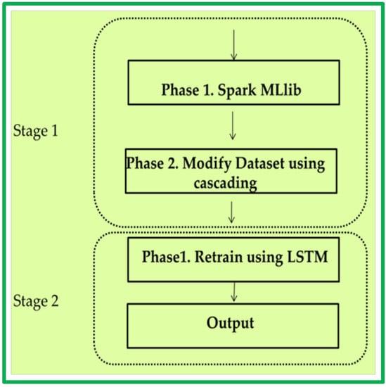
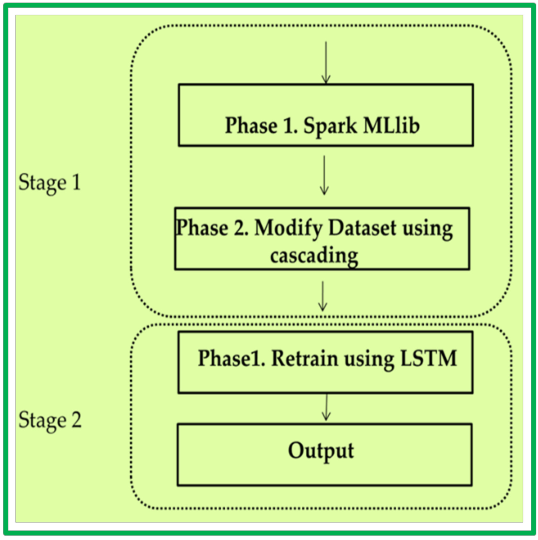
Figure 3 shows the proposed framework structure. It contains two learning stages, outlined as follows.

Stage 1

(i)

Phase 1: big data analysis using Spark MLlib

(ii)

Phase 2: Cascading

Stage 2

(i)

Retrain the model using MLP and LSTM

(ii)

Output

The proposed approach combines advantages from the efficient Spark MLlib with DL, using MLP and LSTM on high dimensional data. The following subsections explain each step in detail.

3.1. Overview of the Architecture

The proposed architecture focuses on determining real-life high dimensional big data problems, utilizing a massive data analysis framework (Spark, Hadoop) and AI (ML, DL). Harnessing such problems is not easy, due to time and space constraints. Big data currently has very large, and growing, volumes but still requires high powered computing equipment to support learning architectures that can manage the data efficiently, utilizing specific resources.

The proposed framework used endeavors to conquer these challenges by cascading the Spark MLlib data analytics framework with MLP and LSTM. The core architecture framework presented here forms the root of the experiment, where the key concept is to utilize cascading between Spark MLlib and DL using MLP and LSTM networks.

3.2. Phase 1. Big Data Processing Using Spark MLlib

Several ML methods were considered in relation to the massive data volumes. We chose the efficient Spark MLlib to implement a support vector machine (SVM), decision tree (DT), random forest (RF) and logistic regression (LR) classifiers. Preprocessed data was passed through these classifiers to generate regression models that introduce the possibility of every data position relating to the binary class. This is the binary learning step.

The SVM classifier is a supervised ML algorithm to classify linear and nonlinear data using hyper-planes [45,46,47] and is appropriate for classification or regression. The concept is to draw the optimal hyperplane that dynamically separates two classes. The separator should be selected such that it provides the maximum margin among vectors of the two classes; hence SVM is also known as the maximal margin classifier. Vectors close to the active hyper-plane are identified as support vectors, as shown in Figure 4 [45,48].

The SVM assumes that a larger margin on the hyperplane will provide superior generalization for data classification. Consider the training vector that represents the binary classes as (x_i, y_i), I = 1 … 1, x_i €Rⁿ, y_i€{+1,−1} where Rⁿ is the input space, x_i is the feature vectors, and y_i is the class label of x_i [45]. The linear separating function can be expressed as:

f(x) = w^tx + b

(10)

where w and b are weight and bias, respectively. The optimal hyper plane margin can be defined as $\frac{2}{{\parallel \mathrm{w}\parallel }^2}$ and the optimization issue can be handled by optimizing the hyper plane,

$${}_{\mathrm{w},\mathrm{b},\in }{}^{\min }\frac{1}{2}\left|\mathrm{w}\right|+\mathrm{C}.$$

(11)

Subject to

$${\mathrm{y}}_{\mathrm{i}}({\mathrm{w}}^{\mathrm{T}}{\mathrm{x}}_{\mathrm{i}})+\mathrm{b}\ge 1-{\in }_{\mathrm{i}},{\in }_{\mathrm{i}}\ge 0$$

(12)

Or its dual issue

$${\min }_{\mathsf{\alpha }}\frac{1}{2}{\mathsf{\alpha }}^{\mathrm{T}}{\mathrm{Q}}_{\mathsf{\alpha }}-{\mathrm{e}}^{\mathrm{T}}\mathsf{\alpha }$$

(13)

Subject to

$$0\le {\mathsf{\alpha }}_{\mathrm{i}}\le \mathrm{C},\mathrm{i}=1\dots 1,{\mathrm{y}}^{\mathrm{T}}\mathsf{\alpha }=0$$

(14)

where e represents a vector of all ones. The penalty parameter, C > 0, is also known as the penalty error. The decision problem can be classified after obtaining α and b by solving Equations (11)–(14) [49],

$$\mathrm{f}(\mathrm{x})={{\displaystyle \sum }}_{\mathrm{i}=1}^1{\mathsf{\alpha }}_{\mathrm{i}}{\mathrm{y}}_{\mathrm{i}}<{\mathrm{x}}_{\mathrm{i},}{\mathrm{x}}_{\mathrm{j}}>+\mathrm{b}$$

(15)

The hyperplane divides the dataset into two classes when it is available in a linearly separable format. It is somewhat difficult to map non-linear separable data into high dimensional space, so SVM utilizes the kernel function to overcome this problem. Kernel functions can be separated into two main categories. Local kernel functions assume data points are near each other, whereas global kernel functions assume data points are distant. These features impact on kernel points.

Table 1. Common support vector machine kernels [49].

Kernel Function	Expression
Linear	K(${\mathrm{x}}_{\mathrm{i}},{\mathrm{x}}_{\mathrm{j}})=1+{\mathrm{x}}_{\mathrm{i}}^{\mathrm{T}}{\mathrm{x}}_{\mathrm{j}}$
Polynomial	K(${\mathrm{x}}_{\mathrm{i}},{\mathrm{x}}_{\mathrm{j}})={(1+{\mathrm{x}}_{\mathrm{i}}^{\mathrm{T}}{\mathrm{x}}_{\mathrm{j}})}^{\mathrm{p}}$
Radial Basis	K(${\mathrm{x}}_{\mathrm{i}},{\mathrm{x}}_{\mathrm{j}})=\exp (-\mathsf{\gamma }{\parallel {\mathrm{x}}_{\mathrm{i}}-{\mathrm{x}}_{\mathrm{j}}\parallel }^2)$
Exponential radial basis	K(${\mathrm{x}}_{\mathrm{i}},{\mathrm{x}}_{\mathrm{j}})=\exp (\frac{-\parallel {\mathrm{x}}_{\mathrm{i}}-{\mathrm{x}}_{\mathrm{j}}\parallel }{2_{\mathsf{\sigma }}^2})$
Gaussian radial basis	K(${\mathrm{x}}_{\mathrm{i}},{\mathrm{x}}_{\mathrm{j}})=\exp (-\frac{{\parallel {\mathrm{x}}_{\mathrm{i}}-{\mathrm{x}}_{\mathrm{j}}\parallel }^2}{2_{\mathsf{\sigma }}^2})$
Sigmoid	K(${\mathrm{x}}_{\mathrm{i}},{\mathrm{x}}_{\mathrm{j}})=\tanh ({\mathrm{kx}}_{\mathrm{i}}^{\mathrm{T}}{\mathrm{x}}_{\mathrm{j}}-\mathsf{\delta }$)

shows various commonly employed kernel functions.

The radial basis function (RBF) provides better performance compared with linear and polynomial kernel functions. SVM classification is popular for high dimensional data spaces. In contrast to ANNs, SVM has no local optima and uses a different kernel function for decision. One of the largest SVM challenges is to choose the most suitable kernel function.

Bermen [50,51] proposed RF in 1999, which is suitable for classification and regression. It is a non-linear classifier that employs DT ensembles to avoid overfitting and has been employed for various classification problems [52,53].

RF contains a group of tree-structured classifiers (T (X, ($\mathsf{\Theta }$m), m = 1 …, where uniformly independent distributed random vectors are represented by ($\mathsf{\Theta }$m), and every tree casts a single vote for the dominant public class at input x. RF is the most prominent data mining ML technique. Every tree in RF is generated by choosing a bootstrap sample.

A few variables are selected at random at each individual internal tree node and used to search for the best partition. Trees are generated on the new dataset to their highest depth without pruning. This procedure is repeated to design new trees in the forest and finally, voting is used to find class labels. The Gini index [54] is commonly employed when searching for the best partition,

$$\mathrm{Gini}={\mathrm{n}}_{\mathrm{L}}{{\displaystyle \sum }}_{\mathrm{k}=1,\dots ,}{\mathrm{k}}_{\mathrm{pkL}}(1-\mathrm{pkL})+{\mathrm{n}}_{\mathrm{R}}{{\displaystyle \sum }}_{\mathrm{k}=1,\dots ,}{\mathrm{k}}_{\mathrm{pkl}}(1-\mathrm{pkR})$$

(16)

where PKL and PKR are the proportion of the class $K$ in the left node and in the right node respectively.

Decision tree is a well-known data mining and ML tool, that produces a tree-like structure containing intermediate test and leaf nodes. Every test node represents boundary of data space and every leaf node represents a class. DT is helpful for data classification and regression (CART) [53,55], where DT boundaries partition the original space into a set of disjoint regions. DT structure recursively divides the data space to build disjoint groups of points to maximize intragroup and minimize intergroup homogeneity. Homogeneity measures differ between the algorithms. CART algorithms [53] mostly uses the GINI impurity, ID3 and C4.5 use information gain [56], and variance reduction is mostly used for regression.

To select optimal splitting points between current splitting points, we need to know the information gain of the splitting points, which is most essential for finding splitting points. Information gain plays a significant role, as more information can be gained from the splitting point as the information gain increases and vice versa [57]. Information gain is derived from impurity differences among parent nodes and a weighted sum of the left and right child nodes. Gini impurity is most commonly employed for classification scenarios:

$${{\displaystyle \sum }}_{\mathrm{i}=1}^{\mathrm{c}}{\mathrm{f}}_{\mathrm{i}}(1-{\mathrm{f}}_{\mathrm{i}})$$

(17)

where ${\mathrm{f}}_{\mathrm{i}}$ ith label frequency at a specific node and C is the number of distinct labels. Entropy was recently proposed for node impurity [57],

$${{\displaystyle \sum }}_{\mathrm{i}=1}^{\mathrm{c}}-{\mathrm{f}}_{\mathrm{i}}\log ({\mathrm{f}}_{\mathrm{i}})$$

(18)

The most popular method used for regression tree impurity is variance,

$$\frac{1}{\mathrm{N}}{\displaystyle \sum }_{\mathrm{i}=1}^{\mathrm{N}}{({\mathrm{y}}_{\mathrm{i}}-\mathsf{\mu })}^2$$

(19)

where ${\mathrm{y}}_{\mathrm{i}}$ and N are the instances and their count, respectively; and μ is the mean. After computing parent node impurity and the weighted sum of the left and right child nodes, information gain can be expressed as,

$$\mathrm{IG}(\mathrm{D},\mathrm{S})=\mathrm{impurity}(\mathrm{D})-\frac{{\mathrm{N}}_{\mathrm{left}}}{\mathrm{N}}\mathrm{impurity}({\mathrm{D}}_{\mathrm{left}})-\frac{{\mathrm{N}}_{\mathrm{right}}}{\mathrm{N}}\mathrm{impurity}({\mathrm{D}}_{\mathrm{right}}).$$

(20)

Logistic regression is a well-known binary classification algorithm with categorical dependent features and has been applied to many applications in biomedical informatics, medical decision support, risk estimation, disease categorization, computer vision, marketing, etc. [58]. LR evaluates data statistically and contains one or more independent variables with vital roles to reflect an outcome. Output is calculated through a variable, and input data is coded as 0 or 1 [59]. LR usually estimates the probability of event occurrence by fitting data to the logit function, which can be solved easily by calculating the β parameters,

$$\mathrm{y}=\{\begin{array}{c}1,\mathsf{\beta }0+\mathsf{\beta }1(\mathrm{x})+\in >0\\ 0,\mathrm{otherwise}\end{array}$$

(21)

where $\in$ is the standard logistic distributed error and β0 and β1 coefficients are generated by calculating the odds ratios among the various groups or categories. The main reason for LR popularity and convenience is that it always provides output between 0 and 1 for any real input t [60].The logistic function g(z) is described as below,

$$\mathrm{g}(\mathrm{z})=\frac{{\mathrm{e}}^{\mathrm{t}}}{{\mathrm{e}}^{\mathrm{t}}+1}=\frac{1}{1+{\mathrm{e}}^{-\mathrm{t}}}$$

(22)

Thus, to implement LR on the multi-class cardiac arrhythmia dataset we first assign the instances between to class 1 or NOT-1, where class 1 included all the instances labeled as “class 01 label” and NOT-1 included all other instances. The main reason for this data classification is that almost 50% of the data belonged to class 1 [61].

We then proceeded as follows:

• The key Spark abstraction was due to RDD so input preprocessed data in the form of RDD.
• Convert the resilient distributed dataset into a data frame.
• Read labels and features from the data frame.
• Non-numeric features having one hot encoding.
• Each encoded feature having string indexing.
• Create vector assembly non-numeric features and one hot encoded feature.
• Alter the assembly vector in the pipeline.
• Modify the pipeline to an appropriate format for Spark.
• Train the model on the training data using the Spark MLlib.

Binary prediction can be obtained by testing whole data.

3.3. Phase 2. Cascading

Cascading is pivotal in the proposed framework to link the prediction data to the primary dataset. We used the modified dataset from stage 2 (knowledge = prediction + original dataset) to train the MLP and LSTM.

3.4. Stage 2. Deep Learning

• This is the second and final framework learning stage before output. We train the MLP and LSTM using the modified dataset from cascading.
• MLP and LSTM can be formed by either reusing steps 2–8 in stage 1, substituting ML for MLP using the Spark library, or MLP could be formed from the ANN initially.
• MLP can be trained using a high-quality training back-propagation algorithm to minimize the errors in prediction.

Various parts of this structure have been used previously in different big data and ML areas, e.g., classification structure and recommendation tools.

3.5. Framework Underlying Logic

The framework architecture described above resolves conventional ML issues, considering all ML conditions, while enhancing accuracy as well as system speed to address big data problems. The main logic underlying the framework is discussed below.

3.5.1. Computation Time

The proposed framework reduces computation time efficiently. Running the two-layer method using two DL models would be lengthy and tedious, and somewhat difficult to ensure outcome quality.

To address computation time problems, we employed fast and efficient big data analysis frameworks, Hadoop or Spark, rather than two DL simultaneous models. Spark includes MLlib, which is particularly appropriate for iterative ML tasks, significantly reducing computation time, as compared with conventional ML approaches.

3.5.2. Feature Set Enhancement

Using the cascade modified dataset as input for the subsequent stages improves framework accuracy. Hence, applying the DL model to the modified data set enhances the feature set.

3.5.3. Continuous Learning Improvement

The proposed framework second stage DL combines MLP and LSTM, training the model via back-propagation. Hence, the model continuously learns new features unsupervised. This allows for the framework to quickly develop as a more accurate and reliable model. The back propagation learning process retains the train prototype, enhance prediction accuracy.

4. Proposed Framework Implementation

This section discusses implementing the proposed framework described in Section 3 as a proof of concept. We first describe the dataset employed and then show the two-step implementation.

The general goal of this experiment was to qualitatively and quantitatively study big data analysis execution, using the proposed structure. Experimental outcomes are described in Section 5.

4.1. Description of the Dataset

We used two different datasets to simulate the implementation and experimental results: (i) Cardiac Arrhythmia Database; (ii) Uniform Resource Locator (URL) Reputation Dataset from University of California Irvine Machine Learning (UCI ML) Repository [62,63].

The Cardiac Arrhythmia Database contains 452 instances or rows, where each row is the medical record for a distinct patient. There are 279 patient attributes, including age, weight, height, patient electrocardiogram (ECG) data, etc. The goal was to classify the data for the presence or absence of cardiac arrhythmia into 16 classes. Class 01 denoted a normal ECG absent of arrhythmia; classes 02 to 15 denoted different arrhythmia types and class 16 denoted unlabeled patients.

The majority of the dataset was biased towards no arrhythmia, with 245 instances corresponding to class 01, 185 instances split between the 14 arrhythmia classes, and the remaining 22 instances being unclassified. About 3 classes did not appear in the dataset referred to the degree of AV block. Dataset labels were supplied by professional cardiologists and they are considered to be the gold model.

The key issue in processing the dataset was the inadequate number of training examples related to a number of features, heavily biased toward no arrhythmia, disappear feature values about (0.333%) and feature values corresponds to both continuous and categorical categories. In short, it is a multiclass classification problem.

However, while this dataset is high dimensional, it does not fulfill the big data requirements. Thus, the URL Reputation Dataset is used, which is an Anonymized 120-day subset of the international conference on Machine learning (ICML-09) URL data containing 2.4 million (i.e., 2,396,130) samples and 3.2 million (i.e., 3,231,961) features.

This dataset fulfills the big data criteria in terms of high dimensionality, volume, and veracity, which makes it suitable for analytics using our Spark based framework. To be more specific, using this dataset, we intend to construct a real-time system that uses machine learning techniques to detect malicious URLs (spam, phishing, exploits, and so on).

To this end, we have explored techniques that involve classifying URLs based on their lexical and host-based features, as well as online learning to process large numbers of examples and adapt quickly to evolving URLs over time.

The task was to identify whether a given sample corresponds to a malicious URL and/or to a benign URL. In short, it is a binary classification problem.

4.2. Cardiac Arrhythmia Classification

To show the proposed approach effectiveness, first, we classified cardiac arrhythmia using linear, tree ensemble, and deep architecture progressively using cascading. Specifically, we first employed LR to assess prediction accuracy and then used DT to classify the data. We then applied RF, as described in Section 3.2 followed by MLP and then LSTM deep architectures, which modeled the dataset more accurately.

Using Spark MLlib-based LR, DT, RF and MLP classifiers, the following steps were performed to prepare training and test sets.

• All 279 cardiac arrhythmia attributes were organized as numerical values using the numerical columns.
• The vector assembler was utilized to join all 279 attributes within individual vectors for all Spark MLlib based algorithms. This vector feature located below features in the data frame.
• As discussed above, the dataset included 16 arrhythmia classes, with the presence or absence represented as 1 and 0, respectively.

Once the dataset was prepared, we randomly split 80% for the training and 20% for the test datasets. We trained LR, DT and RF classifiers using the training set and evaluated prediction accuracy using the test set, applying 10-fold cross-validation to identify the best hyperparameters.

Assuming the training data consisted of p arrhythmia types for each group x_i, we have a set Y(x_i) of actual arrhythmia type and a set G(x_i) of predicted arrhythmia type generated by the classifier. Therefore, if the set arrhythmia type labels or classes is L = $\{{\mathrm{l}}_0$,${\mathrm{l}}_1$, …, ${\mathrm{l}}_{\mathrm{M}-1}$}, then the true output vector y will have N elements such that y₀, y₁, …, y_N−1 ∈ L.

We then trained the LR, DT and RF classifiers, which take a single sample and generate a prediction vector by minimizing cross-entropy of the true versus predicted distributions, $\widehat{\mathrm{Y}}$ = (yˆ0, yˆ1, …, yˆN − 1 ∈ L. When training the classifiers, keeping the test and validation sets separate enables us to learn the model hyper-parameters [43]. Thus, we can calculate the confusion matrix elements for the multiclass classification problem as,

$${\mathrm{C}}_{\mathrm{ij}}={{\displaystyle \sum }}_{\mathrm{K}=0}^{\mathrm{N}-1}\widehat{\mathsf{\delta }}({\mathrm{y}}_{\mathrm{k}}-{\mathrm{l}}_{\mathrm{i}})·\widehat{\mathsf{\delta }}({\widehat{\mathrm{Y}}}_{\mathrm{k}}-{\mathrm{l}}_{\mathrm{j}})$$

(23)

where

$$\widehat{\mathsf{\delta }}(\mathrm{x})=\{\begin{array}{cc}1& \mathrm{if}\mathrm{x}=0,\\ 0& \mathrm{otherwise}\end{array}.$$

(24)

Then ${\mathrm{C}}_{\mathrm{ij}}$ can be used to compute performance metrics, such as weighted precision, ${\mathrm{PPV}}_{\mathrm{w}}$, weighted recall, ${\mathrm{TPR}}_{\mathrm{w}}$, and weighted F1 value, Fw$(\mathsf{\beta })$, for the predicted against true population labels,

$${\mathrm{PPV}}_{\mathrm{w}}=\frac{1}{\mathrm{N}}{{\displaystyle \sum }}_{\mathrm{l}\in \mathrm{L}}\mathrm{PPV}(\ell )·{{\displaystyle \sum }}_{\mathrm{i}=0}^{\mathrm{N}-1}\hat{\mathsf{\delta }}({\mathrm{y}}_{\mathrm{i}}-\mathrm{l})$$

(25)

$${\mathrm{TPR}}_{\mathrm{w}}=\frac{1}{\mathrm{N}}{{\displaystyle \sum }}_{\mathrm{l}\in \mathrm{L}}\mathrm{TPR}(\ell )·{{\displaystyle \sum }}_{\mathrm{i}=0}^{\mathrm{N}-1}\widehat{\mathsf{\delta }}({\mathrm{y}}_{\mathrm{i}}-\mathrm{l})$$

(26)

and

$${\mathrm{F}}_{\mathrm{W}}(\mathsf{\beta })=\frac{1}{\mathrm{N}}{{\displaystyle \sum }}_{\mathrm{l}\in \mathrm{L}}\mathrm{F}(\mathsf{\beta },\ell )·{{\displaystyle \sum }}_{\mathrm{i}=0}^{\mathrm{N}-1}\widehat{\mathsf{\delta }}({\mathrm{y}}_{\mathrm{i}}-\mathrm{l})$$

(27)

Respectively, we also calculated the network root mean square error,

$$\mathrm{RMSE}=\sqrt{\frac{{{\displaystyle \sum }}_{\mathrm{i}=0}^{\mathrm{N}-1}{({\mathrm{y}}_{\mathrm{i}}-{\widehat{\mathrm{y}}}_{\mathrm{i}})}^2}{\mathrm{N}}}$$

(28)

Finally, when the training was completed, the trained model was used to score against the test set to measure predicted groups versus variants producing a confusion matrix for the performance in a multiclass setting using Equation (23).

In stage 2, we further classified the dataset using MLP and LSTM incrementally. First; we train MLP with the following subsequent attributes:

• input layer contained 281 units,
• two hidden layers with 64 units each and a sigmoid activation function,
• output layer with Softmax activation function having 2 units.

The back-propagation accompanied by the logistic loss function had a vital role in training the complete network. Training was performed using different epoch sizes.

However, we could not perform cross-validation with MLP since the current implementation did not provide this functionality. The confusion matrix, precision, recall, F1-score, and RMSE were calculated as described for LR, DT and RF models above.

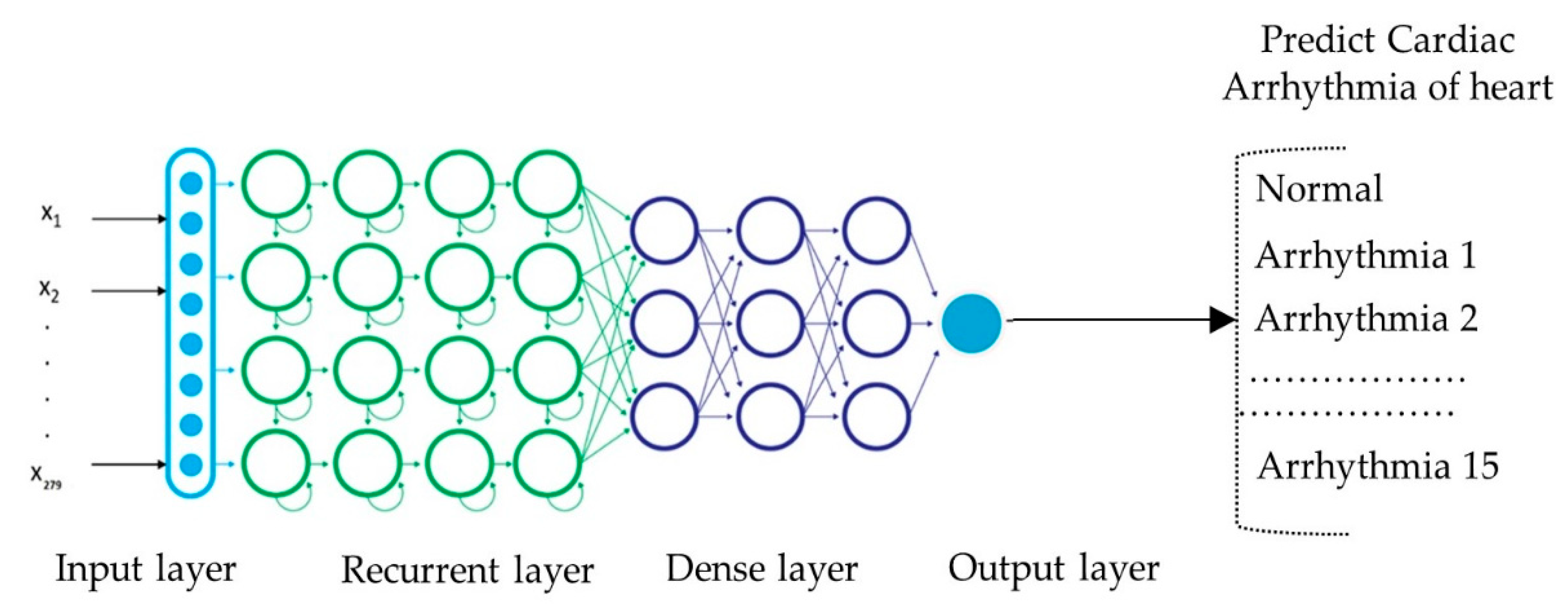
Stage 2 prediction using LSTM was the last predictive model. Before we started training the LSTM network, we converted the Spark data frame into sequence format, so it could be fed into the LSTM network. We then randomly split the sequence data into train, test, and validation sets 60%, 20% and 20%, respectively.

Figure 5 shows the LSTM network for distinguishing cardiac arrhythmia presence and absence into the 16 groups. The network consisted of an input layer, 4 LSTM layers, 3 dense layers, and an output layer. The input consisted of ECG signal sequences and took an input sequence x_t at time step t and computed the hidden state, h_t.

We then trained the LSTM network, which takes a single sequence at each time step, generating a prediction vector by minimizing cross-entropy of the true versus predicted distributions yˆ = ˆy0, ˆy1, …, ˆyN − 1 $\in$ L. When training the network, keeping the test and validation set separate enables us to learn hyper-parameters for the model [43].

We used the ADADELTA adaptive learning rate algorithm to automatically combine the gain of learning rate annealing and momentum training to prevent slow LSTM network convergence. The ReLU activation function was employed in the LSTM layers for better regularization, and drop out probability was set to 0.9 to avoid overfitting.

Softmax activation function was used in the output layer to provide the probability distribution over the classes. The confusion matrix, precision; recall, F1-score, and root-mean-square error (RMSE) were calculated as for LR, DT and RF. Finally, the model total score and accuracy was achieved.

4.3. Identifying Malicious URLs

To show the effectiveness of the proposed approach on a larger dataset, further, we carried out another experiment for identifying malicious URLs for online using linear, tree ensemble, and deep architecture progressively using cascading. Specifically, we first employed LR to assess prediction accuracy and then used DT to classify the data. We then applied RF followed by MLP and then LSTM deep architectures, which modeled the dataset more accurately.

Using Spark MLlib based LR, DT, RF and MLP classifiers, the following steps were performed to prepare training and test sets.

• All 3,231,961 lexical and host-based features were organized as numerical values using the numerical columns.
• The vector assembler was utilized to join all 3,231,961 attributes within individual vectors for all Spark MLlib based algorithms. This vector feature was located below features in the data frame.
• As discussed above, the dataset included 2classes, with either as malicious URL or as a benign URL represented as 1 and 0, respectively.

Once the dataset was prepared, we randomly split 80% for the training and 20% for the test datasets. We trained LR, DT and RF classifiers (i.e., such as arrhythmia, but as a binary classification setting) using the training set, and evaluated prediction accuracy using the test set, applying 10-fold cross-validation to identify the best hyperparameters.

Finally, when the training was completed, the trained model was used to score against the test set to measure predicted groups versus variants, producing a confusion matrix for the performance in a multiclass setting using Equation (23).

In stage 2, we further classified the dataset using MLP and LSTM incrementally. First; we train MLP with the following subsequent attributes:

• input layer contained 3,231,960 units,
• three hidden layers with 128, 256 and 512 units each and a sigmoid activation function,
• output layer with Softmax activation function having 2 units.

The back-propagation accompanied by the logistic loss function had a vital role in training the complete network. Training was performed using different epoch sizes.

Stage 2 prediction using LSTM was the last predictive model, where the input set is randomly split the sequence data into the train, test, and validation sets 60%, 20% and 20%, respectively.

Similar to the cardiac arrhythmia dataset, we again used the ADADELTA adaptive learning rate algorithm to automatically combine the gain of learning rate annealing and momentum training to prevent slow LSTM network convergence. The ReLU activation function was employed in the LSTM layers for better regularization and drop out probability was set to 0.7 to avoid overfitting. Softmax activation function was used in the output layer to provide the probability distribution over the classes.

Since the second experiment is about solving a binary classification problem, the Matthews correlation coefficient (MCC) [64], Area under the receiver operating characteristic (ROC) curve and area under the precision-recall curve were used as the measure of the quality of binary classifications. The MCC takes into account true and false positives and negatives and is generally regarded as a balanced measure which can be used even if the classes are of very different sizes.

The MCC is, in essence, a correlation coefficient between the observed and predicted binary classifications; it returns a value between −1 and +1. A coefficient of +1 represents a perfect prediction, 0 no better than random prediction and −1 indicates total disagreement between prediction and observation.

While there is no perfect way of describing the confusion matrix of true and false positives and negatives by a single number, the Matthews correlation coefficient is generally regarded as being one of the best of such measures. The MCC can be calculated directly from the confusion matrix using the formula:

$$\mathrm{MCC}=\frac{\mathrm{TP}\ast \mathrm{TN}-\mathrm{FP}\ast \mathrm{FN}}{\sqrt{(\mathrm{TP}+\mathrm{FP})(\mathrm{TP}+\mathrm{FN})(\mathrm{TN}+\mathrm{FP})(\mathrm{TP}+\mathrm{FN})}}$$

(29)

Finally, the total score and accuracy of the model were achieved in terms of MCC, Area under the receiver operating characteristic (ROC) curve and area under the precision-recall curve.

5. Experimental Results

In this section, we illustrate experimental results based on the experimental settings described in Section 4.

5.1. Experimental Setup

To show the effectiveness of our proposed approach on both datasets, we implemented the first stage in Scala using Spark MLlib as the ML platform. The LSTM networks, on the other hand, were implemented in Java using the Deeplearning4j DL framework in both cases.

Experiments were performed on a computing cluster with 32 cores running 64-bit Ubuntu 14.04 OS. The software stack consisted of Apache Spark v2.3.0, Java (JDK) 1.8, Scala 2.11.8 and Deeplearning4j 1.0.0. alpha. The LSTM network was trained on a Nvidia TitanX GPU with CUDA and cuDNN enabled to improve overall pipeline speed.

5.2. Stage 1 Classification Analysis

As discussed in Section 4, we implemented the proposed framework in two steps. Step 1 classified cardiac arrhythmia and URL Reputation Dataset using LR, DT and RF, with outcomes as shown in

Table 2. Classifier outcomes at stage 1 for Cardiac arrhythmia Dataset.

Classifier	Accuracy	Precision	Recall	F1-score
LR	83.0%	83.0%	82.3%	83.0%
DT	85.4%	86.2%	87.5%	86.5%
RF	87.5%	86.0%	87.0%	87.0%

and

Table 3. Classifier outcomes at stage 1 for URL Reputation Dataset.

Classifier	Accuracy	auPR	auROC	MCC
LR	85%	88%	85%	0.73
DT	92%	92%	92%	0.85
RF	93%	93.4%	93.5%	0.87

respectively.

The logistic regression classifier exhibits poor performance since the feature spaces were large (279 and 3231961 dimensions respectively. Since the Cardiac Arrhythmia dataset also had a number of categorical features, the logistic regression classifier could not handle them very well. Nevertheless, it depends on the transformations for non-linear features and depends on whole data.

Tree-based approaches (DT and RF) rely on intuitive decision rules and hence can deal with non-linear features. Nevertheless, they consider variable interactions.

Both DT and RF perform better than LR in all metrics. RF is a versatile algorithm and can be expected to outperform LR on many medium-sized tasks. It can also handle categorical and real-valued features with ease, with little to no preprocessing required. With proper cross-validation technique, they are readily tuned.

Thus, tree-based approaches provide an effective arsenal to analyze this high dimensional dataset. Since RF performance was slightly superior to DT, we chose the RF outcome to propagate into the next stage.

5.3. Stage 2 Classification Analysis

The second stage again classified both the cardiac arrhythmia and URL Reputation Datasets but by using deep learning architectures: MLP and LSTM. The performance metrics are shown in

Table 4. Performance metrics of deep learning models for the cardiac arrhythmia dataset.

Classifier	Accuracy	Precision	Recall	F1-score
MLP	89.0%	88.0%	89.0%	88.3%
LSTM	94.8%	96.0%	96.7%	96.2%

and

Table 5. Performance metrics of deep learning models for URL Reputation Dataset.

Classifier	Accuracy	auPR	auROC	MCC
MLP	95%	96%	95%	0.91
LSTM	96%	97%	96%	0.94

respectively. MLP did not perform well, since the feature space is very large (i.e., 279 dimensions). The accuracy score on the training set went above 95% in the training step, but we achieved approximately 88% accuracy for the test set. Thus, MLP had an overfitting problem in this case.

Therefore, later on, we trained LSTM to see if it could overcome the overfitting. LSTM modeled long-short-term dependencies very well, performing better than all other classifiers in all metrics.

In summary, linear and tree-based approaches (stage 1) and LSTM (stage 2) provide an effective arsenal to analyze this high dimensional dataset. Since LSTM performed much better than RF or MLP, the overall outcome was generated from the LSTM to accurately predict arrhythmia probability.

Table 6. Proposed and previous models’ prediction accuracy for the cardiac arrhythmia dataset.

Method	Accuracy	Reference
Supervised ML algorithms	62.0%	[62]
Classifier comparison	66.9%	[67]
Different ML approaches	72.7%	[61]
SVM and KNN	73.8%	[65]
OneR, J48, and Naïve Bayes	74.7%	[68]
Wrapper algorithm	78.2%	[66]
Various search algorithms	81.0%	[69]
Proposed Framework	94.8%

shows that the proposed approach achieved superior classification accuracy than previous approaches. As the table demonstrates, Fazel et al. [61] used several ML techniques and achieved an accuracy of 72.7%; Guvenir et al. [62] developed the VF15 ML algorithm and achieved 62% accuracy; Niazi et al. [65] used SVM and K nearest neighbors to achieve an accuracy of 68% and 73.8%, respectively.

Mustaqeem et al. [66] selected the best features using a wrapper algorithm around various ML classifiers and achieved 78.2% accuracy. Samad et al. [67] used different ML classifiers and achieved 66.9% accuracy; Soman et al. [68] used One R, J48, and Naïve Bayes ML techniques and achieved 74.7% highest accuracy.

Persada et al. [69] used various search methods and achieved 81% maximum accuracy with the Best First search. Thus, the proposed model offers significantly improved cardiac arrhythmia classification accuracy compared with previous models.

According to the authors of [64], using MCC, a correlation of +1 indicates perfect agreement, 0 is expected for a prediction no better than random, and −1 indicates total disagreement between prediction and observation. In all our cases for the 2nd dataset, MCC shows a very strong positive relationship (i.e., >+0.7), which means most of the classifier managed to extract the relationships between features (see Table 3 and Table 5).

On the other hand, the higher the Area under the precision-recall curve (auPR) and Area under the receiver operating characteristic (ROC) curve (auROC), the better the models were. Fortunately, both of these values are significantly higher, which show that our classifier performed well. The dataset is slightly imbalanced, so we used auPR as the performance metric along with auROC too (see Table 3 and Table 5).

6. Conclusions and Outlook

In this manuscript, we proposed an efficient framework to perform big data analytics in an accurate and scalable way. Our proposed approach combined Apache Spark and DL beneath the ML umbrella and provided significantly superior results compared to state-of-the-art approaches.

Using the two-stage cascading architecture, our frameworks managed to solve both multiclass and binary classification problems with an acceptable level of accuracy.

The proposed two-step big data analysis framework was capable of processing a massive amount of data tasks over a very short computational time, with less computational complexity and with significantly higher accuracies for both datasets, the Cardiac arrhythmia and URL Reputation dataset, respectively.

In the future, we intend to extend the framework by considering more factors and parameters to solve other real-life research problems with robust deep architectures.

References

- Nair, L.R.; Shetty, S.D. Applying spark based machine learning model on streaming big data for health status prediction. Comput. Electr. Eng. 2018, 65, 393–399. [Google Scholar] [CrossRef]
- Hbibi, L.; Barka, H. Big data: Framework and issues. In Proceedings of the 2016 International Conference on Electrical and Information Technologies (ICEIT 2016), Tangier, Morocco, 4–7 May 2016. [Google Scholar]
- Assefi, M.; Behravesh, E.; Liu, G.; Tafti, A.P. Big data machine learning using apache spark MLlib. In Proceedings of the 2017 IEEE International Conference on Big Data, Boston, MA, USA, 11–14 December 2017. [Google Scholar]
- Abbasi, A.; Sarker, S.; Chiang, R.H. Big data research in information systems: Toward an inclusive research agenda. J Assoc. Inf. Syst. 2016, 17, 1–33. [Google Scholar] [CrossRef]
- Fu, J.; Sun, J.; Wang, K. Spark—A big data processing platform for machine learning. In Proceedings of the 2016 Conference on Industrial Informatics-Computing Technology, Intelligent Technology, Industrial Information Integration (ICIICII 2016), Wuhan, China, 3–4 December 2016. [Google Scholar]
- Richter, A.N.; Khoshgoftaar, T.M.; Landset, S.; Hasanin, T. A multi-dimensional comparison of toolkits for machine learning with big data. In Proceedings of the 2015 IEEE International Conference on Information Reuse and Integration (IRI 2015), San Francisco, CA, USA, 13–15 August 2015. [Google Scholar]
- Karim, M.R.; Alla, S. Scala and Spark for Big Data Analytics: Explore the Concepts of Functional Programming, Data Streaming, and Machine Learning; Packt Publishing Ltd.: Birmingham, UK, 2017. [Google Scholar]
- Longadge, R.; Dongre, S. Class imbalance problem in data mining review. arXiv 2013, arXiv:1305.1707. [Google Scholar]
- Rahman, F.; Slepian, M.; Mitra, A. A novel big-data processing framwork for healthcare applications: Big-data-healthcare-in-a-box. In Proceedings of the 2016 IEEE International Conference on Big Data, Washington, DC, USA, 5–8 December 2016. [Google Scholar]
- Archenaa, J.; Anita, E.M. Interactive big data management in healthcare using spark. In Proceedings of the 3rd International Symposium on Big Data and Cloud Computing Challenges (ISBCC 2016), Chennai, India, 10–11 March 2016. [Google Scholar]
- Tafti, A.P.; LaRose, E.; Badger, J.C.; Kleiman, R.; Peissig, P. Machine learning-as-a-service and its application to medical informatics. In Proceedings of the 2017 International Conference on Machine Learning and Data Mining in Pattern Recognition, New York, NY, USA, 15–20 July 2017. [Google Scholar]
- Van Horn, J.D. Opinion: Big data biomedicine offers big higher education opportunities. Proc. Natl. Acad. Sci. USA 2016, 113, 6322–6324. [Google Scholar] [CrossRef] [PubMed] [Green Version]
- Anisetti, M.; Ardagna, C.; Bellandi, V.; Cremonini, M.; Frati, F.; Damiani, E. Privacy-aware big data analytics as a service for public health policies in smart cities. Sustain. Cities Soc. 2018, 39, 68–77. [Google Scholar] [CrossRef]
- Rios, E.; Prünster, B.; Suzic, B.; Carnehult, T.; Prieto, E.; Notario, N.; Suciu, G.; Ruiz, J.F.; Orue-Echevarria, L.; Rak, M.; et al. Cloud technology options towards Free Flow Of Data. DPSP Cluster 2017. Available online: http://www.diva-portal.org/smash/record.jsf?pid=diva2%3A1232492&dswid=-865 (accessed on 15 June 2018). [CrossRef]
- Lau, B.P.L.; Wijerathne, N.; Ng, B.K.K.; Yuen, C. Sensor fusion for public space utilization monitoring in a smart city. IEEE Internet Things J. 2018, 5, 473–481. [Google Scholar] [CrossRef]
- Apache Spark Lightning-Fast Unified Analytics Engine. Available online: http://spark.apache.org/ (accessed on 7 July 2018).
- Barquero, J.B. Getting Started with Spark. Available online: http://malsolo.com/blog4java/?p=679 (accessed on 15 June 2018).
- Zaharia, M.; Chowdhury, M.; Das, T.; Dave, A.; Ma, J.; McCauley, M.; Franklin, M.J.; Shenker, S.; Stoica, I. Resilient distributed datasets: A fault-tolerant abstraction for in-memory cluster computing. In Proceedings of the 9th USENIX conference on Networked Systems Design and Implementation, San Jose, CA, USA, 25–27 April 2012. [Google Scholar]
- Apache Spark Mllib. Available online: http://spark.apache.org/mllib (accessed on 15 May 2018).
- Soomro, T.R.; Shoro, A.G. Big Data Analysis: Apache Spark Perspective. Glob. J. Comput. Sci. Technol. 2015, 15, 7–14. [Google Scholar]
- Meng, X.; Bradley, J.; Yavuz, B.; Sparks, E.; Venkataraman, S.; Liu, D.; Freeman, J.; Tsai, D.B.; Amde, M.; Owen, S.; et al. Mllib: Machine learning in apache spark. J. Mach. Learn. Res. 2016, 17, 1235–1241. [Google Scholar]
- Community Effort Driving Standardization of ApacheSpark through Expanded Role in Hadoop Project, Cloudera, Databricks, IBM, Intel, and Map R, OpenSource Standards. Available online: https://www.cloudera.com/more/news-and-blogs/press-releases/2014-07-01-community-effort-driving-standardization-of-apache-spark-through.html (accessed on 15 June 2018).
- Zaharia, M.; Xin, R.S.; Wendell, P.; Das, T.; Armbrust, M.; Dave, A.; Meng, X.; Rosen, J.; Venkataraman, S.; Franklin, M.J.; et al. Apache spark: A unified engine for big data processing. Commun. ACM 2016, 59, 56–65. [Google Scholar] [CrossRef]
- Github-Apache Spark. Available online: https://github.com/apache/spark/ (accessed on 15 July 2018).
- Nair, L.R.; Shetty, S.D. Streaming twitter data analysis using sparkfor effective job search. J. Theor. Appl. Inf. Technol. 2015, 80, 349. [Google Scholar]
- Nodarakis, N.; Sioutas, S.; Tsakalidis, A.; Tzimas, G. Large scale sentiment analysis on Twitter with Spark. In Proceedings of the Workshop EDBT/ICDT Joint Conference, Bordeaux, France, 15 March 2016. [Google Scholar]
- Shyam, R.; Ganesh, H.B.; Kumar, S.; Prabaharan, P.; Soman, K.P. Apache Spark a big data analytics platform for smart grid. Procedia Technol. 2015, 21, 171–178. [Google Scholar] [CrossRef]
- Yousefi, N.; Georgiopoulos, M.; Anagnostopoulos, G.C. Multi-task learning with group-specific feature space sharing. In Proceedings of the Joint European Conference on Machine Learning and Knowledge Discovery in Databases, Porto, Portugal, 7–11 September 2015; pp. 120–136. [Google Scholar]
- Fazli, M.S.; Vella, S.A.; Moreno, S.N.J.; Quinn, S. Computational motility tracking of calcium dynamics in toxoplasma gondii. arXiv 2017, arXiv:1305.1707. [Google Scholar]
- Allahyari, M.; Pouriyeh, S.; Assefi, M.; Safaei, S.; Trippe, E.D.; Gutierrez, J.B.; Kochut, K. A brief survey of text mining: Classification, clustering and extraction techniques. arXiv 2017, arXiv:1707.02919. [Google Scholar]
- Gandomi, A.; Haider, M. Beyond the hype: Big data concepts, methods, and analytics. Int. J. Inf. Manag. 2015, 35, 137–144. [Google Scholar] [CrossRef]
- Krawczyk, B. Learning from imbalanced data: Open challenges and future directions. Prog. Artif. Intell. 2016, 5, 221–232. [Google Scholar] [CrossRef]
- Prati, R.C.; Batista, G.E.; Silva, D.F. Class imbalance revisited: A new experimental setup to assess the performance of treatment methods. Knowl. Inf. Syst. 2015, 45, 247–270. [Google Scholar] [CrossRef]
- Kotsiantis, S.; Kanellopoulos, D.; Pintelas, P. Handling imbalanced datasets: A review. GESTS Int. Trans. Comput. Sci. Eng. 2006, 30, 25–36. [Google Scholar]
- Sonak, A.; Patankar, R.; Pise, N. A new approach for handling imbalanced dataset using ANN and genetic algorithm. In Proceedings of the 2016 International Conference on Communication and Signal Processing (ICCSP 2016), Chennai, India, 6–8 April 2016. [Google Scholar]
- Popescu, M.C.; Sasu, L.M. Feature extraction, feature selection and machine learning for image classification: A case study. In Proceedings of the 2014 International on Optimization of Electrical and Electronic Equipment (OPTIM 2014), Brasov, Romania, 22–24 May 2014. [Google Scholar]
- Silva, L.M.J.; Marques de Sá, J.; Alexandre, L.A. Data classification with multilayer perceptrons using a generalized error function. Neural Netw. 2008, 21, 1302–1310. [Google Scholar] [CrossRef] [PubMed]
- Zanaty, E. Support vector machines (SVMs) versus multilayer perception (MLP) in data classification. Egypt. Inf. J. 2012, 13, 177–183. [Google Scholar] [CrossRef]
- Sharma, C. Big Data Analytics Using Neural Networks. Master’s Thesis, San José State University, San José, CA, USA, May 2014. [Google Scholar]
- Sarwar, S.M.; Hasan, M.; Ignatov, D.I. Two-stage cascaded classifier for purchase prediction. arXiv 2015, arXiv:1508.03856. [Google Scholar]
- Simonovsky, M.; Komodakis, N. Onionnet: Sharing features in cascaded deep classifiers. arXiv 2016, arXiv:1608.02728. [Google Scholar]
- Long, J.; Shelhamer, E.; Darrell, T. Fully convolutional networks for semantic segmentation. In Proceedings of the 2015 IEEE Conference on Computer Vision and Pattern Recognition, Boston, MA, USA, 7–12 June 2015. [Google Scholar]
- Karim, M.; Cochez, M.; Beyan, O.D.; Zappa, A.; Sahay, R.; Decker, S.; Schuhmann, D.-R. Recurrent deep embedding networks for genotype clustering and ethnicity prediction. arXiv 2018, arXiv:1805.12218. [Google Scholar]
- Kang, D.; Lv, Y.; Chen, Y.-Y. Short-term traffic flow prediction with LSTM recurrent neural network. In Proceedings of the 2017 IEEE 20th International Conference on Intelligent Transportation Systems (ITSC), Yokohama, Japan, 16–19 October 2017. [Google Scholar]
- Priyadarshini, A. A map reduce based support vector machine for big data classification. Int. J. Database Theory Appl. 2015, 8, 77–98. [Google Scholar] [CrossRef]
- Vapnik, V. The Nature of Statistical Learning Theory; Springer: Berlin, Germany, 2013. [Google Scholar]
- Gunn, S.R. Support vector machines for classification and regression. ISIS Tech. Rep. 1998, 14, 5–16. [Google Scholar]
- Tomar, D.; Agarwal, S. A comparison on multi-class classification methods based on least squares twin support vector machine. Knowl.-Based Syst. 2015, 81, 131–147. [Google Scholar] [CrossRef]
- Jakkula, V. Tutorial on support vector machine (SVM). School EECS 2006, 37, 1–13. [Google Scholar]
- Singh, V.; Gupta, R.; Sevakula, R.K.; Verma, N.K. Comparative analysis of Gaussian mixture model, logistic regression and random forest for big data classification using map reduce. In Proceedings of the 2016 11th International Conference on Industrial and Information Systems (ICIIS 2016), Roorkee, India, 3–4 December 2016. [Google Scholar]
- Breiman, L. Random forests. Mach. Learn. 2001, 45, 5–32. [Google Scholar] [CrossRef]
- Biau, G. Analysis of a random forests model. J. Mach. Learn. Res. 2012, 13, 1063–1095. [Google Scholar]
- Breiman, L.; Friedman, J.; Stone, C.J.; Olshen, R.A. Classification and Regression Trees; CRC Press: Boca Raton, FL, USA, 1984. [Google Scholar]
- Farris, F.A. The Gini index and measures of inequality. Am. Math. Mon. 2010, 117, 851–864. [Google Scholar] [CrossRef]
- Giannakopoulos, I.; Tsoumakos, D.; Koziris, N. A decision tree based approach towards adaptive modeling of big data applications. In Proceedings of the 2017 IEEE International Conference on Big Data, Boston, MA, USA, 11–14 December 2017. [Google Scholar]
- Quinlan, J.R. Induction of decision trees. Mach. Learn. 1986, 1, 81–106. [Google Scholar] [CrossRef] [Green Version]
- Wisesa, H.A.; Ma’sum, M.A.; Mursanto, P.; Febrian, A. Processing big data with decision trees: A case study in large traffic data. In Proceedings of the 2016 International Workshop on Big Data and Information Security (IWBIS 2016), Jakarta, Indonesia, 18 October 2018. [Google Scholar]
- Jiang, Y.; Hamer, J.; Wang, C.; Jiang, X.; Kim, M.; Song, Y.; Xia, Y.; Mohamed, N.; Sadat, M.N.; Wang, S. SecureLR: Secure logistic regression model via a hybrid cryptographic protocol. IEEE/ACM Trans. Comput. Biol. Bioinform. 2018, 1. [Google Scholar] [CrossRef] [PubMed]
- Sharma, M.; Shukla, S. Relative object localization using logistic regression. In Proceedings of the 2017 3rd International Conference on Advances in Computing, Communication & Automation (ICACCA), Dehradun, India, 15–16 September 2017. [Google Scholar]
- Kobayashi, F.; Eram, A.; Talburt, J. Entity resolution using logistic regression as an extension to the rule-based oyster system. In Proceedings of the 2018 IEEE Conference on Multimedia Information Processing and Retrieval (MIPR), Miami, FL, USA, 10–12 April 2018. [Google Scholar]
- Fazel, A.; Algharbi, F.; Haider, B. Classification of Cardiac Arrhythmias Patients. CS229 Final Project Report. 2014. Available online: http://cs229.stanford.edu/proj2014/AlGharbi%20Fatema,%20Fazel%20Azar,%20Haider%20Batool,%20Cardiac%20Arrhythmias%20Patients.pdf (accessed on 15 July 2018).
- Guvenir, H.A.; Acar, B.; Demiroz, G.; Cekin, A. Supervised machine learning algorithm for arrhythmia analysis. IEEE Comput. Cardiol. 1997, 24, 433–436. [Google Scholar]
- Ma, J.; Saul, L.K.; Savage, S.; Voelker, G.M. Identifying suspicious URLs: An application of large-scale online learning. In Proceedings of the 26th Annual International Conference on Machine Learning, Montreal, QC, Canada, 14–18 June 2009. [Google Scholar]
- Matthews, B.W. Comparison of the predicted and observed secondary structure of T4 phage lysozyme. Biochim. Biophys. Acta (BBA) Protein Struct. 1975, 405, 442–451. [Google Scholar] [CrossRef]
- Niazi, K.A.; Khan, S.A.; Shaukat, A.; Akhtar, M. Identifying best feature subset for cardiac arrhythmia classification. In Proceedings of the Science and Information Conference (SAI 2015), London, UK, 28–30 July 2015; pp. 494–499. [Google Scholar]
- Mustaqeem, A.; Anwar, S.M.; Majid, M.; Khan, R.K. Wrapper method for feature selection to classify cardiac arrhythmia. In Proceedings of the 2017 39th Annual International Conference of the IEEE Engineering in Medicine and Biology Society (EMBC 2017), Jeju Island, Korea, 11–15 July 2017. [Google Scholar]
- Samad, S.; Khan, S.A.; Haq, A.; Riaz, A. Classification of arrhythmia. Int. J. Electr. Energy 2014, 2, 57–61. [Google Scholar] [CrossRef]
- Soman, T.; Bobbie, P.O. Classification of arrhythmia using machine learning techniques. WSEAS Trans. Comput. 2005, 4, 548–552. [Google Scholar]
- Persada, A.G.; Setiawan, N.A.; Nugroho, H.A. Comparative study of attribute reduction on arrhythmia classification dataset. In Proceedings of the 2013 International Conference on Information Technology and Electrical Engineering (ICITEE 2013), Yogyakarta, Indonesia, 7–8 October 2013. [Google Scholar]
Figure 1.
(a) Apache Spark ecosystem and (b) Apache Spark MLlib development [21].
Figure 2.
A typical long short-term memory cell [43].
Figure 3.
A macro view of the stages in our proposed big data analytics framework.
Figure 4.
Support vectors and margins [45].
Figure 5.
Recurrent Long Short-Term Memory (LSTM) model.