Abstract
Compared with ordinary image classification tasks, fine-grained image classification is closer to real-life scenes. Its key point is how to find the local areas with sufficient discrimination and perform effective feature learning. Based on a bilinear convolutional neural network (B-CNN), this paper designs a local importance representation convolutional neural network (LIR-CNN) model, which can be divided into three parts. Firstly, the super-pixel segmentation convolution method is used for the input layer of the model. It allows the model to receive images of different sizes and fully considers the complex geometric deformation of the images. Then, we replaced the standard convolution of B-CNN with the proposed local importance representation convolution. It can score each local area of the image using learning to distinguish their importance. Finally, channelwise convolution is proposed and it plays an important role in balancing lightweight network and classification accuracy. Experimental results on the benchmark datasets (e.g., CUB-200-2011, FGVC-Aircraft, and Stanford Cars) showed that the LIR-CNN model had good performance in fine-grained image classification tasks.
1. Introduction
Fine-grained image classification has been one of the most popular research topics in the fields of computer vision and pattern recognition in recent years [1,2,3]. The purpose of fine-grained image classification is to divide images of large categories into sub-category images, such as different types of birds, aircrafts, cars, and so on. One can easily conclude that fine-grained image classification has a very broad range of research needs and application prospects in both academic research and daily life. Meanwhile, subtle differences between classes and large differences within classes are the major features of fine-grained images. Therefore, fine-grained image classification is more difficult than ordinary image classification. The successful application of neural networks in medicine [4], mining science [5], roughness prediction [6], and microwave modeling [7,8,9] has pointed us in their direction. The long-term development of deep learning [10] has provided us with solutions.
Fine-grained image classification is a research task with both needs and challenges. The signal-to-noise ratio of fine-grained images is very small. How to accurately locate effective local areas to extract features with sufficient discrimination has become a trendy research topic. Most of the related algorithms mentioned in this paper are based on deep convolution features. These methods can be roughly divided into two types: algorithms based on strong supervision and algorithms based on weak supervision. In the model training stage, the algorithms based on strong supervision greatly improve the classification accuracy of fine-grained image classification [11,12,13,14]. In addition to the category labels for images, these algorithms also use additional manual annotations, including bounding box and part locations. However, the acquisition of manual annotation information is very expensive, which greatly limits the practicality of such algorithms. Recently, weakly supervised classification algorithms that use only category labels to complete classification tasks have been becoming increasingly mature. Some advanced weakly supervised classification algorithms achieve or exceed many classification algorithms that rely on manual annotation.
Finding valid local area information is a vital step for fine-grained image classification algorithms. Weakly supervised classification algorithms such as constellations [15], ST-CNN [16], and MG-CNN [17] improve the classification accuracy by detecting and locating these local regions using a convolutional neural network (CNN). From another perspective, this paper chooses not to directly detect and locate local regions, but gives each region a different importance through self-learning. The proposed method is called local importance representation convolution (LIR-convolution). First, we use the convolution operation to learn how important each local area of an image (i.e., receptive field) is to the classification results. Then, we assign these importance factors to the corresponding image regions to enhance the features of important regions and suppress noise. The main line of LIR-convolution is to extract valid features, and the secondary line of LIR-convolution assigns different weights to the extracted features. This learning approach simplifies the algorithm flow and makes the algorithm more efficient.
The image sizes in fine-grained image datasets vary widely. This is especially true for images in actual scenes. For CNNs, we need to normalize the images to the same size. In most cases, we use cropping [18] and scaling [19] to achieve this effect. SPP-Net [20] adopts the spatial pyramid pooling method after the last convolutional layer to skillfully transfer features of the same size to the fully-connected layer. However, inputting images of the same size will be more conducive to batch operations on the network. Authors in [21] proposed DCN, a deformable convolution operation to adapt to image geometry deformation problems. In addition, DCN contributes the concept of non-fixed geometric convolution kernels. Inspired by this, we proposed the super-pixel segmentation convolution (SPS-convolution) method. It convolves the images to the same size by performing simple clustering on the image datasets. This is equivalent to a pre-processing convolution operation.
The large number of parameters of the CNN guarantees the powerful representational ability of the model. However, as the depth of the network increases, the complexity of the model becomes higher and higher. How to design a lightweight model is a bottleneck that CNN research needs to solve in practical applications. Xception [22], MobileNet [23], etc. have made great progress in designing lightweight models. However, for fine-grained image classification, the excessive reduction of model parameters can result in the network not being able to learn more discriminative features. This paper proposes a channelwise convolution approach to achieve a good balance between lightweight model and classification accuracy. In contrast to traditional convolution and depthwise convolution [24], channelwise convolution means sliding on the feature channels with a certain size of receptive field.
2. Related Work
2.1. Weak Supervised Classification Model
How to locate effective local areas and extract sufficient features is the key which influences algorithm success. Berg [25], Perronnin [26], and other researchers improved the accuracy of positioning with specific handmade algorithms, and the classification result was raised to about 60%. However, due to the limited ability to express features, the early “artificial feature-based algorithms” did not get enough ideal classification results. So, we need to implement a more refined local positioning function and a more powerful feature description approach. In recent years, neural networks and deep learning has achieved great success in signal detection [27,28,29] and image processing [30,31,32]. Using deep CNNs for fine-grained image classification has become a popular research route.
With the rapid development of deep learning, classification algorithms based on weak supervision have become a major trend in fine-grained image classification. A two-level attention model [33] was the first attempt to complete fine-grained image classification tasks using only category labels. Firstly, it employs a convolutional network to filter the background image and get multiple candidate regions with foreground objects. Secondly, the features of each candidate region are extracted using an object-level model. Then, the above features are clustered using a part-level model to obtain a region detector. Finally, the local region of the test sample is detected using this region detector. A bilinear CNN [34] is a bilinear recognition model consisting of two feature extractors based on a CNN. It uses only image labels for end-to-end training. Discriminative region localization and fine-grained feature learning are two challenges for fine-grained image classification. All of the above methods address these two challenges independently. RA-CNN [35] comprises three sub-networks of different scales. Each sub-network further includes two types of networks—a classification network and an APN network. The article allows two types of networks to recursively learn in a mutually reinforcing manner. MA-CNN [36] is a new part-learning algorithm where feature learning and part generation can reinforce each other. It generates more discriminative parts from feature channels and learns better fine-grained features from parts in a mutually reinforcing manner. DFL-CNN [37] heightens mid-level representation learning within the CNN’s architecture. It captures class-specific discriminative patches by learning a set of convolution filters. Such filter banks have properly initialized, discriminatively learned, and well-structured characteristics. Experimental results show that these methods implement the state-of-the-art on fine-grained recognition datasets. SENet [38] adopts a novel “feature recalibration” strategy. It obtains the importance of each feature channel by self-learning. Then, the important factors are multiplied to the corresponding channels. SENet won the image classification mission of the last ImageNet competition. Inspired by SENet, The LIR-convolution we propose first acquires the importance of each receptive field by self-learning. Then, these important factors are assigned to the corresponding parts of feature maps.
2.2. Lightweight Convolution Model
The CNN’s structure moves toward being deeper, wider, and more lightweight. Deep CNNs can abstract low-level data into high-level patterns. In theory, deeper (number of network layers) and wider (number of neurons) networks can learn more complex features. Nevertheless, pure “depth tuning” can lead to over-fitting, high computational complexity, and vanishing gradient problems. The inception family [39,40,41,42] reduces parameters while increasing the depth and width of the network. Moreover, they also increase the adaptability of the network to different scales. The ResNet architecture [43,44] adds “skip connections” to enable the network to train deeper and faster. The challenge of fine-grained image recognition requires a deeper and wider network. On the contrary, its adaptability to actual scenes requires a more lightweight network. With convolution and pooling structures, the CNN itself is a simplified neural network. NIN [45] greatly reduces network parameters by using global average pooling and “1 × 1” convolution operations. For memory reasons, AlexNet [46] employs group convolution skills first. Group convolution operations can significantly reduce parameters, but there is a lack of information interaction between each group of channels. IGCNet [47] subtly achieves the purpose of interlaced feature complementation through two sets of convolution operations (i.e., group convolution and interleaved group convolution). Both Xception [22] and MobileNet [23] draw on depthwise separable convolution skills to promote the separation of spatial convolution and channel convolution. The depthwise and pointwise convolution operations can vastly reduce the complexity of the model. The creators of ShuffleNet [48] felt that pointwise convolution still has a lot of redundant parameters, and it was proposed to utilize pointwise group convolution and channel shuffle instead of pointwise convolution. These networks reduce the complexity of the model and achieve good results on coarse-grained image datasets. However, for fine-grained images, local features with discrimination are more difficult to extract, and overly simplified convolution parameters will affect the recognition rate of classification. Based on this, we propose a channelwise convolution operation. To make a comparison, the ordinary convolution performs a sliding operation on the receptive field, but the channelwise convolution carries out the sliding behavior on the channel with a certain stride. This can not only meet the requirements of reducing parameters, but also fully increases the information interaction between channels. Channelwise convolution allows us to strike a balance between building lightweight networks and getting enough features.
3. Approach
3.1. Local Importance Representation Convolution
The key point of fine-grained image classification is finding some local areas with subtle differences. A common and effective method is to detect foreground objects and discover important regional information. This section focuses on the ability to distinguish the spatial dimension information of images, and proposes local importance representational convolution (LIR-convolution). LIR-convolution obtains the importance factor of each local area by self-learning, and then selectively enhances the beneficial local area and suppresses useless local areas according to these importance factors. The CNN obtains global information by aggregating local information on the local receptive field layer-by-layer. Given the local characteristics of the local receptive field itself, we let LIR-convolution learn the importance of the local receptive field. The structure of LIR-convolution is shown in Figure 1.
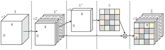
Figure 1.
The structure schematic of the local importance representation convolution (LIR-convolution) method.
Figure 1 is divided into four sections by broken lines. The first part is the process of completing X to X’ by ordinary convolution operations. “c1” and “c2” represent the number of channels of X and X’, respectively. V = [, , …, ] denote the set of convolution kernels used for X to X’.
Here ⊙ represents a convolution operation, = [, , …, ] and X = [, , …, ], while denotes a single channel of . The second part implements the transformation of X’ to U’. Depthwise separable convolution is employed to further convolve features and reduce the training parameters. Then, the ReLU activation function is used, which makes the feature more nonlinear:
V’ denotes the set of convolution kernels used for X’ to U’. c3 represents the number of channels of U’. V’ = [’, ’, …, ’] and U’ = [’, ’, …, ’]. The third part realizes the conversion of U’ to U. By channel compression of the feature maps, we get a two-dimensional feature map. Then, we use the sigmoid activation function to activate the feature map to get a two-dimensional table with values between 0 and 1:
V″ denotes the set of convolution kernels used for U’ to U. V″ = [″, ″, …, ″] and U = []. We performed one kind of convolution operation using a convolution kernel with the same number of channels as the feature maps. U records the importance of each location of the image. Next, we assign the local importance recorded in U to the corresponding local area of the feature maps received by LIR-convolution.
where ⊗ represents each feature channel of X’ multiplied by U. X are feature maps with local importance representationally obtained by LIR-convolution processing.
3.2. Super-Pixel Segmentation Convolution
In this section, we present a convolution operation based on super-pixel segmentation, called SPS-convolution. The images are segmented by the improved simple linear iterative clustering (improved SLIC) method to obtain the specified number of super-pixels, and each super-pixel contains the same number of pixels. Each super-pixel is a set of adjacent pixels with similar properties. Then, we adopt a convolution operation for the super-pixels by turn. After that, we can conduct the unified processing of the input images without worrying about their different sizes. Note that the image blocks after super-pixel segmentation have their own geometric meanings. Compared with the fixed geometry convolution kernels of standard CNNs, SPS-convolution is easier to adapt to the complex geometric transformation of images. A detailed introduction to the SPS-convolution is provided in the following and the comparison of four different convolution algorithms is shown in Figure 2.
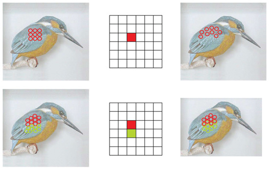
Figure 2.
Four kinds of convolution methods for a convolutional neural network (CNN). Top-left: The traditional convolution operation. It has fixed geometry convolution kernels (e.g., a rectangular convolution kernel with side lengths m and n). Top-right: The deformable convolution operation. It adjusts the shape of the convolution kernel based on the geometric deformation of the object. However, it does not adequately consider the spatial relationship inside the object. Bottom-left: The super-pixel segmentation convolution (SPS-convolution) operation. It first clusters the pixels and then convolves the resulting super-pixels. It can simultaneously consider the geometric deformation and spatial relationship of an object. Bottom-right: The SPS-convolution operation (Version 2). Based on the original super-pixel segmentation method, it is allowed to have overlapping regions between super-pixels obtained by clustering. The SPS-convolution (Version 2) makes the network adapt to different sizes of input.
SPS-convolution limits the size of each super-pixel and allows overlapping regions between super-pixels. We set the height and width of the input image to be H and W, and each super-pixel contains k pixels. Another two parameters need to be set: the quantity of super-pixels K and the compact coefficient m. The algorithm steps are as follows:
- Generate K seed points on the input image. The distance of the adjacent seed points on the vertical axis and the horizontal axis are and :
- Calculate the gradient values for all pixels in the 3 × 3 neighborhood of the seed point, and move the seed point to the place where the gradient is the smallest.
- Calculate the distance D between each pixel in the 2 × 2 neighborhood of the seed point and the seed point. The computation formulae are:where l, a, b are from the CIELAB color space and x, y are from its position information, is the CIELAB color space color difference value, is the distance between pixels, i and j represent two pixels, m is the compact coefficient, and s is the maximum spatial distance within the class.
- Each super-pixel block is composed of k pixels, which are around the seed point and distances (D) between them are smallest. One pixel can belong to different super-pixels.
- Go back to Step 2 and perform multiple iteration optimizations. The number of iterations is I. We will get K super-pixels, and each super-pixel size is k.
- The convolution operation will be performed on each super-pixel, and the convolution stride is . That is to say, each convolution kernel is convolved only once for each super-pixel.
3.3. Channelwise Convolution
Channelwise convolution is a convolution operation between traditional convolution and group convolution (the depthwise convolution can be regarded as the ultimate group convolution). Channelwise convolution allows the convolution kernels to perform sliding convolution operations on the feature channels in the form of sliding groups. This idea mimics the behavior of the convolution kernels sliding on the feature maps. For channelwise convolution, the sliding window sizes are w × h, the sliding step is s, and the number of channels spanned by performing one convolution operation is c. Channelwise convolution can control the number of parameters and computational complexity by setting s and c, and increasing the relationship among channels under parameter-controlled conditions. The channelwise convolution diagram is shown in Figure 3.
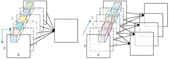
Figure 3.
The schematic on the left shows the standard convolution operation. During convolution, the convolution kernel moves right and down along the receptive field. The schematic on the right shows the channelwise convolution method. In the course of convolution, the convolution kernel moves in the direction of the channel.
As shown in Figure 3, the convolution kernel of a standard convolution operation is a three-dimensional block. The size of the third dimension is equal to the number of channels (C) of the feature map. Decoupling standard convolution kernels is deepwise convolution kernels, which means that the kernel of deepwise convolution is a two-dimensional block. The kernel of the channelwise convolution method is also a three-dimensional block, but the size c of the third dimension is smaller than C. The channelwise convolution kernel is slid on the channels with stride s. As long as the values of c and s are reasonably adjusted, the relationship between the feature channels can be maximized and the amount of parameters can be reduced. Compared to depthwise convolution and group convolution, it pays more attention to the information interaction between channels.
3.4. LIR-CNN Model
The final version of LIR-CNN model is a bilinear convolutional neural network (B-CNN) structure that introduces SPS-convolution, LIR-convolution, and channelwise convolution. The first three sections describe these three operations in detail. Among them, SPS-convolution flexibly convolves the input images to the same sizes. LIR-convolution learns the importance of each local area of the image. Channelwise convolution is designed to balance network performance and parameter complexity. The flowchart of the LIR-CNN model is shown in Figure 4.
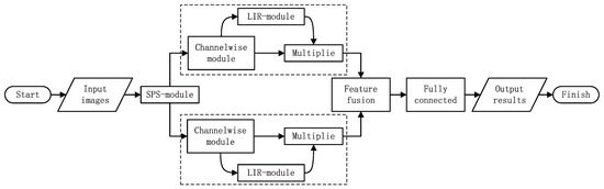
Figure 4.
Flowchart of the LIR-CNN model.
As shown in Figure 4, “SPS-module”, “LIR-module”, and “Channelwise module” represent modules that contain the three convolution methods, respectively. In addition to the proposed convolution methods, these modules include pooling operations, activation functions, and so on. First, the model receives input images and transmits them to the bilinear branches after SPS-module processing. Each branch is composed of multiple “Channelwise modules” and “LIR-modules”. That is, the dashed box is linearly connected by modules of similar structure. The features from the two paths are aggregated by sun-pooling technology, and then processed by the fully connected layer and the softmax layer to finally output the results.
4. Experiments
We performed experiments on three fine-grained image datasets, including CUB-200-2011 (birds) [49], FGVC-Aircraft (aircrafts) [50], and Stanford Cars (cars) [51]. The birds dataset consists of 11,788 images in 200 categories. This dataset is split into 5994 training images and 5794 test images. The aircrafts dataset consisting of 10,000 images has 6667 training images and 3333 test images, and 100 categories. The cars dataset comprises 8144 training images and 8041 test images. This dataset consists of 16,185 images and contains a total of 196 categories. Figure 5 shows partial examples of the three datasets, and Figure 6 shows the different states of images during the operation of the LIR-CNN model.
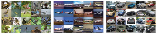
Figure 5.
Examples from the CUB-200-2011 [49] dataset (left), FGVC-Aircraft [50] dataset (center), and Stanford Cars [51] dataset (right).
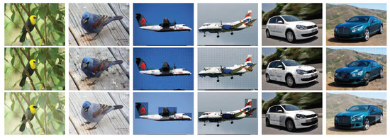
Figure 6.
Schematic diagram of the intermediate process of image processing by the LIR-CNN model. The input images are displayed in the first line, the super-pixel-segmented images are placed on the second line, and the schematic diagram with the importance factors assigned are shown in the third line.
Lin [34] et al. have demonstrated that a bilinear network model is superior to a single network model, and an asymmetric network structure is better than a symmetric network structure. Therefore, our experiments adopted the structure of B-CNN [D, M], where D and M represent D-Net [52] and M-Net [53] respectively. Both modules were pre-trained by the ImageNet dataset and the softmax layer of the network was reconstructed according to the number of categories of the datasets. We initialized the network with the conv5 layer of M-net and the conv5_3 layer of D-Net, and fine-tuned the network with a small learning rate. The input images were first resized to 448 × 448 and the features were extracted through two networks. Bilinear features of size 512 × 512 were obtained by sum-pooling and normalization. The bilinear feature was finally adjusted to a bilinear vector and the classifier was used for image classification. The simple structure of M-Net and D-Net is shown in Table 1.

Table 1.
The simple structure of M-Net and D-Net.
4.1. LIR-CNN_V1
The standard convolution in the B-CNN structure was replaced by the LIR-convolution module to form the bilinear LIR-CNN, referred to as LIR-CNN_V1. Figure 7 shows the structures of the standard convolution and LIR-convolution. During the experiment, all five M-Net convolutional layers were replaced with LIR-convolution, and D-Net’s conv1_2, conv2_2, conv3_3, conv4_3, and conv5_3 layers were replaced with LIR-convolution. “Separable Conv” stands for the depthwise separable convolution [22,23] operation. After the first separable convolution operation, the feature channels become c3. In the experiments, c3 took the values 1, 20, and c2, respectively. After the second separable convolution operation, the feature channel was reduced to 1. Then, through the sigmoid operation, a two-dimensional local importance matrix was obtained, and finally the value of the matrix was assigned to the position corresponding to the image. The experimental results are shown in Table 2.
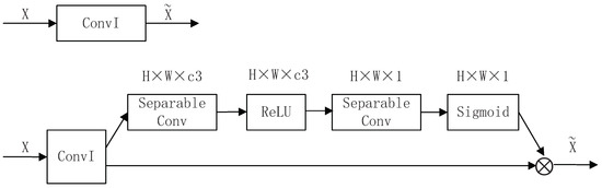
Figure 7.
The diagram on the top shows the ordinary convolution operation, and the schematic on the bottom shows the local importance representation convolution structure. “ConvI” expresses the convolutional layers in Table 1.
Table 2.
The classification accuracy of different models on three datasets, and the convolutional layers’ parameter increments of these models. B-CNN: bilinear CNN.
“△Params” indicates the increment of the parameters of the convolution kernels after the introduction of the LIR-convolution module (compared with B-CNN). B-CNN achieved excellent results in fine-grained image classification, mainly because it employs the modeling of local pairwise features interactions. The second-order feature statistics method makes B-CNN obtain higher-dimensional and finer features. LIR-CNN_V1 (c3 = 20) achieved better experiment results than B-CNN on all three data sets. The classification accuracy on birds, aircrafts, and cars datasets increased by 1%, 1.9%, and 0.3%, respectively. This is because we added a local importance factor to make feature learning more efficient. When c3 = 1, the results of the experiment hardly changed, and the classification accuracy increased by 0.1%, 0.5%, and % on the three datasets, respectively. Mainly because we do not have enough parameters for learning, the learned local importance matrix could not accurately express the importance of local regions of the image for classification. “c3 = c2” indicates that the number of channels of the feature map was not changed during the first separable convolution phase of LIR-convolution. Compared with c3 = 20, the experimental results improved but were not obvious. The feature fusion layer and fully connected layer of LIR-CNN_V1 were identical to B-CNN. The difference between them is the convolution operation. With the increase of the parameters of the convolution kernel, the computational complexity and training time of the network also increased significantly. This can be seen intuitively from the last column of Table 2.
4.2. LIR-CNN_V2
LIR-CNN_V2 preprocesses the input images using SPS-convolution on the basis of LIR-CNN_V1. We provided two sets of experimental data for comparison. They divided the images into 448 × 448 and 224 × 224 super-pixels, respectively. For each super-pixel, the former contained 4 × 4 pixels and the latter had 6 × 6 pixels. The latter method absorbed more pixels to capture richer local features and compensate for the loss of super-pixels reduction. In the experiments, we set the iterations of super-pixel segmentation to 5 and the compact coefficient to 10. This is because we allowed overlapping regions between super-pixels, and their boundaries did not have to be too precise. Then, we performed a convolution operation on each super-pixel, and the convolutional strides were 4 and 6. The sizes of the feature maps obtained by SPS-convolution were 448 × 448 and 224 × 224, respectively. The experimental results are shown in Table 3, where “sp = 448” and “sp = 224” indicate that 448 × 448 and 224 × 224 super-pixels were obtained by segmentation.
Table 3.
The classification accuracy of different models on the three datasets. sp: super-pixels obtained by segmentation.
As can be seen from Table 3, compared with B-CNN, the classification accuracies of LIR-CNN_V2 (sp = 448) on datasets birds, aircrafts, and cars increased by 1.6%, 3.1%, and 0.5%, respectively. Compared with B-CNN_V1, the classification accuracy on the three datasets birds, aircrafts, and cars also increased by 0.4%, 0.9%, and 0.3%. Compared with directly resizing the images, these experimental results are sufficient to show that LIR-CNN_V2 can preserve more original structural information of images by super-pixel segmentation. Compared with “sp = 448”, the classification accuracies of LIR-CNN_V2 did not decrease significantly when “sp = 224”, which means that 224 × 224 super-pixels already contained virtually all image information. We performed super-pixel segmentation before convolution operations on the image. This facilitates full account of the complex geometric deformation of the images. At this point, the classification accuracy of LIR-CNN_V2 (sp = 224) on the birds dataset was slightly lower, which indicates that the birds dataset is more complex. “sp = 224” had little difference in terms of convolutional layer parameters compared with “sp = 448”. However, the former was smaller in size, which greatly reduced the amount of calculation and the training time of the entire network.
4.3. LIR-CNN_V3
In the next experiments, we introduced channelwise convolution to the second version of LIR-CNN, which is LIR-CNN_V3 (CC) (hereinafter referred to as “V3_CC”) in Table 4. This part of the content mainly discusses how to balance the parameter complexity and the classification accuracy of the network. For reference, two additional sets of comparative experiments were provided. We replaced the standard convolution with separable convolution and denoted it as LIR-CNN_V3 (SC) (hereinafter referred to as “V3_SC”) in Table 4. LIR-CNN_V3 (DC+SC) (hereinafter referred to as “V3_DC+CC”) means adding depthwise convolutions before the channelwise convolution of V3_CC. “V3_SC” had the same convolution layers and kernel sizes as the original network, except that it used depthwise separable convolution instead of the standard convolution operation. Channelwise convolution is simple, but not easy to implement. In practice, we adopted the “rotation feature map’s dimension” method to convert its work into “standard convolution from another angle”. As shown in Figure 8, “H”, “W”, and “C” represent the height, width, and number of channels of the image; “h”, “w”, and “c” respectively represent the height, width, and depth of the convolution kernel. First, we split the image into W/w blocks along the channel direction. Then, we rotated the image blocks to get a new image with H as the height, C × W/w as the width, and w as the number of channels. Then, we employed h, c, and w as the height, width, and depth of the convolution kernel, and used this kernel to perform convolution operations along the channel direction of the original image. To facilitate splitting and resizing of the image, for M-Net and D-Net, the values of w were 27 and 28, respectively; c was one third of the channels of the original feature map; the value of h was the same as the value in the standard convolution kernel.
Table 4.
The classification accuracy of different models on three datasets, and the convolutional layers’ parameter increments of these models. CC: channelwise convolution; DC+CC: depthwise convolutions were added before the channelwise convolution; SC: separable convolution.
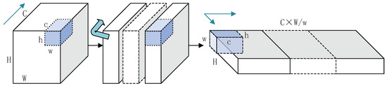
Figure 8.
Diagram of the implementation process of channelwise convolution.
“△Params ” represents the increment of the parameters of the convolution kernels (compared with B-CNN). As shown in the last column of Table 4, a positive value indicates an increase in the number of parameters, and a negative value shows a decrease in the number of parameters. LIR-CNN equipped with channelwise convolution had a good performance on three fine-grained image datasets. Compared with B-CNN, the classification accuracy of “V3_CC” increased by 1.2%, 2.5%, and 0.3% for birds, aircrafts, and cars datasets, respectively. Compared with “LIR-CNN_V2”, the quantity of convolutional parameters of “V3_CC” was reduced by 17.75 M, but its classification accuracy was slightly decreased. This is because channelwise convolution focuses more on information interaction between channels than standard convolution. Compared with “V3_SC”, the number of convolutional parameters of “V3_CC” increased by 0.81 M, but its classification accuracy increased by 0.5%, 1.1%, and 0.4%, respectively. This also shows that the high performance of separable convolution in ordinary image recognition was not fully reflected in fine-grained image classification. Compared with “LIR-CNN_V2”, the classification accuracy of “V3_DC+SC” increased by 0.4%, 0.5%, and 0.2%, respectively. At the same time, the quantity of convolutional parameters of “V3_DC+SC” was also reduced by 17.43 M. The “V3_DC+SC” model takes full account of spatial correlations and cross-channel correlations. This model further reduces the number of parameters in favor of reducing training time.
5. Conclusions
In this paper, we highlight the learnability of the local importance of the image. The LIR-CNN model derives the importance of each receptive field through self-learning and assigns these important factors to the corresponding parts of the image. This allows the model to locate effective local regions and extract enough features. We effectively improved the input layer and lightweight design of the network. The good performance of the LIR-CNN model in fine-grained image classification tasks proves that it can be used in practical scenes and engineering applications. The SPS-convolution, LIR-convolution, and channelwise convolution methods proposed in this paper have strong adaptability and practicability. These three new convolution methods can be easily grafted into various network structures.
To further illustrate the effectiveness of the LIR-CNN algorithm, we will attempt to visualize the experimental results. Then, we will try to build models for specific application scenarios to meet a wider range of needs. B-CNN proves that the performance of asymmetric networks is better than that of symmetric networks. However, both M-Net and D-Net are linear networks, which are only different in depth. Our future research will try to adopt nonlinear network structures such as ResNet and DenseNet. We will try to extend the second-order feature statistics method of B-CNN to multi-level feature statistics. Next, we will study the fusion of LIR-CNN and the visual attention model to further improve network performance by combining “dynamic learning” and “precise positioning”.
Author Contributions
All authors contributed equally to this paper.
Funding
This work was supported by the National Natural Science Foundation of China (Grant Nos. 61872231, 61703267) and Graduate Student Innovation Project of Shanghai Maritime University 2017ycx083.
Conflicts of Interest
The authors declare no conflicts of interest.
References
- Peng, Y.X.; He, X.T.; Zhao, J.J. Object-Part Attention Model for Fine-Grained Image Classification. IEEE Trans. Image Process. 2018, 27, 1487–1500. [Google Scholar] [CrossRef] [PubMed]
- Zhang, Y.; Lian, J.; Fan, M.Q.; Zheng, Y.J. Deep Indicator for Fine-Grained Classification of Banana’s Ripening Stages. EURASIP J. Image Video Process. 2018, 1, 46. [Google Scholar] [CrossRef]
- Wei, X.S.; Xie, C.W.; Wu, J. Mask-CNN: Localizing Parts and Selecting Descriptors for Fine-Grained image Recognition. Pattern Recogn. 2018, 76, 704–714. [Google Scholar] [CrossRef]
- Koprowski, R.; Lanza, M.; Irregolare, C. Corneal Power Evaluation after Myopic Corneal Refractive Surgery Using Artificial Neural Networks. BioMed. Eng. Online 2016, 15, 121. [Google Scholar] [CrossRef] [PubMed]
- Tadeusiewicz, R. Neural Networks in Mining Sciences-General Overview and Some Representative Examples. Arch. Min. Sci. 2015, 60, 971–984. [Google Scholar] [CrossRef]
- Ganovska, B.; Molitoris, M.; Hosovsky, A.; Pitel, J. Design of the Model for the On-Line Control of the AWJ Technology Based on Neural Networks. Indian J. Eng. Mater. Sci. 2016, 23, 279–287. [Google Scholar]
- Dudczyk, J.; Matuszewski, J.; Wnuk, M. Applying the Relational Modelling and Knowledge Based Techniques to the Emitter Database Design. In Proceedings of the International Conference on Microwaves, Radar and Wireless Communications, Gdańsk, Poland, 20–22 May 2002; pp. 172–175. [Google Scholar]
- Dudczyk, J.; Kawalec, A.; Wnuk, M. Applying the Neural Networks to Formation of Radiation Pattern of Microstrip Antenna. In Proceedings of the International Radar Symposium, Wroclaw, Poland, 21–23 May 2008; pp. 99–102. [Google Scholar]
- Dudczyk, J.; Kawalec, A. Adaptive Forming the Beam Pattern of Microstrip Antenna with the Use of an Artificial Neural Network. Int. J. Antennas Propag. 2012, 2012, 388–392. [Google Scholar] [CrossRef]
- LeCun, Y.; Bengio, G.; Hinton, G. Deep Learning. Nature 2015, 521, 436–444. [Google Scholar] [CrossRef] [PubMed]
- Zhang, N.; Donahue, J.; Girshick, R.; Darrell, T. Part-based R-CNNs for Fine-grained Category Detection. In Proceedings of the European Conference on Computer Vision, Zurich, Switzerland, 6–12 September 2010; pp. 834–849. [Google Scholar]
- Lin, D.; Shen, X.Y.; Lu, C.W.; Jia, J.Y. Deep LAC: Deep localization, alignment and classification for fine-grained recognition. In Proceedings of the IEEE Conference on Computer Vision and Pattern Recognition, Boston, MA, USA, 8–10 June 2015; pp. 1666–1674. [Google Scholar]
- Xu, Z.; Huang, S.L.; Zhang, Y.; Tao, D.C. Augmenting Strong Supervision Using Web Data for Fine-Grained Categorization. In Proceedings of the IEEE International Conference on Computer Vision, Santiago, Chile, 13–16 December 2015; pp. 2524–2532. [Google Scholar]
- Huang, S.L.; Xu, Z.; Tao, D.C.; Zhang, Y. Part-Stacked CNN for Fine-Grained Visual Categorization. In Proceedings of the IEEE Conference on Computer Vision and Pattern Recognition, Las Vegas, NV, USA, 26 June–1 July 2016; pp. 1173–1182. [Google Scholar]
- Simon, M.; Rodner, E. Neural Activation Constellations: Unsupervised Part Model Discovery with Convolutional Networks. In Proceedings of the IEEE International Conference on Computer Vision, Santiago, Chile, 13–16 December 2015; pp. 1143–1151. [Google Scholar]
- Jaderberg, M.; Simonyan, K.; Zisserman, A.; kavukcuogu, K. Spatial transformer networks. In Proceedings of the Advances in Neural Information Processing Systems, Montréal, QC, Canada, 7–12 December 2015; pp. 2017–2025. [Google Scholar]
- Wang, D.Q.; Shen, Z.Q.; Shao, J.; Zhang, W.; Xue, X.Y.; Zhang, Z. Multiple Granularity Descriptors for Fine-Grained Categorization. In Proceedings of the IEEE International Conference on Computer Vision, Santiago, Chile, 13–16 December 2015; pp. 2399–2406. [Google Scholar]
- Zeiler, M.D.; Fergus, R. Visualizing and Understanding Convolutional Networks. In Proceedings of the European Conference on Computer Vision, Zurich, Switzerland, 6–12 September 2014; pp. 818–833. [Google Scholar]
- Girshick, R.; Donahue, J.; Darrell, T.; Malik, J. Rich feature hierarchies for accurate object detection and semantic segmentation. In Proceedings of the IEEE Conference on Computer Vision and Pattern Recognition, Columbus, OH, USA, 24–27 June 2014; pp. 580–587. [Google Scholar]
- He, K.; Zhang, X.; Ren, S.; Sun, J. Spatial Pyramid Pooling in Deep Convolutional Networks for Visual Recognition. IEEE Trans. Pattern Anal. 2015, 37, 1904–1916. [Google Scholar] [CrossRef] [PubMed]
- Dai, J.; Qi, H.; Xiong, Y.; Li, Q.; Zhang, G.D.; Hu, H.; Wei, Y.C. Deformable Convolutional Networks. arXiv, 2017; arXiv:1703.06211. [Google Scholar]
- Chollet, F. Xception: Deep Learning with Depthwise Separable Convolutions. arXiv, 2017; arXiv:1610.02357. [Google Scholar]
- Howard, A.G.; Zhu, M.L.; Chen, B.; Kalenichenko, D.; Wang, W.J.; Weyand, T.; Andreetto, M.; Adam, H. MobileNets: Efficient Convolutional Neural Networks for Mobile Vision Applications. arXiv, 2017; arXiv:1704.04861. [Google Scholar]
- Sifre, L. Rigid-Motion Scattering for Image Classification. Ph.D. Thesis, Ecole Polytechnique, Paris, France, 2014. [Google Scholar]
- Berg, T.; Belhumeur, P.N. POOF: Part-Based One-vs.-One Features for Fine-Grained Categorization, Face Verification, and Attribute Estimation. In Proceedings of the IEEE Conference on Computer Vision and Pattern Recognition, Portland, OR, USA, 23–28 June 2013; pp. 955–962. [Google Scholar]
- Perronnin, F.; Sanchez, J.; Mensink, T. Improving the Fisher Kernel for Large-Scale Image Classification. In Proceedings of the European Conference on Computer Vision, Crete, Greece, 5–11 September 2010; pp. 143–156. [Google Scholar]
- Gajewski, J.; Valis, D. The Determination of Combustion Engine Condition and Reliability Using Oil Analysis by MLP and RBF Neural Networks. Tribol. Int. 2017, 115, 557–572. [Google Scholar] [CrossRef]
- Perronnin, F.; Sanchez, J.; Mensink, T. Neural Network Application for Emitter Identification. In Proceedings of the International Radar Symposium, Prague, Czech, 15–17 August 2017; pp. 1–8. [Google Scholar]
- Glowacz, A. Acoustic Based Fault Diagnosis of Three-Phase Induction Motor. Appl. Acoust. 2018, 137, 82–89. [Google Scholar] [CrossRef]
- Perronnin, F.; Sanchez, J.; Mensink, T. Object Detection and Recognition System Using Artificial Neural Networks and Drones. In Proceedings of the Signal Processing Symposium, Jachranka, Poland, 12–14 September 2017; pp. 1–5. [Google Scholar]
- Ma, B.Y.; Ban, X.J.; Huang, H.Y.; Chen, Y.L.; Liu, W.B.; Zhi, Y.H. Deep Learning-Based Image Segmentation for Al-La Alloy Microscopic Images. Symmetry 2018, 10, 107. [Google Scholar] [CrossRef]
- Zhang, L.; Cheng, Z.X.; Shen, Y.; Wang, D.Q. Palmprint and Palmvein Recognition Based on DCNN and A New Large-Scale Contactless Palmvein Dataset. Symmetry 2018, 10, 78. [Google Scholar] [CrossRef]
- Xiao, T.J.; Xu, Y.C.; Yang, K.Y.; Zhang, J.X.; Peng, Y.X.; Zhang, Z. The application of two-level attention models in deep convolutional neural network for fine-grained image classification. In Proceedings of the IEEE Conference on Computer Vision and Pattern Recognition, Boston, MA, USA, 8–10 June 2015; pp. 842–850. [Google Scholar]
- Lin, T.Y.; RoyChowdhury, A.; Maji, S. Bilinear CNN Models for Fine-grained Visual Recognition. In Proceedings of the IEEE International Conference on Computer Vision, Santiago, Chile, 13–16 December 2015; pp. 1449–1457. [Google Scholar]
- Fu, J.L.; Zheng, H.L.; Mei, T. Look Closer to See Better: Recurrent Attention Convolutional Neural Network for Fine-Grained Image Recognition. In Proceedings of the IEEE Computer Vision and Pattern Recognition, Honolulu, HI, USA, 21–26 July 2017; pp. 4476–4484. [Google Scholar]
- Zheng, H.L.; Fu, J.L.; Mei, T.; Luo, J.B. Learning Multi-Attention Convolutional Neural Network for Fine-Grained Image Recognition. In Proceedings of the IEEE International Conference on Computer Vision, Venice, Italy, 22–29 October 2017; pp. 5219–5227. [Google Scholar]
- Wang, Y.M.; Morariu, V.I.; Davis, L.S. Learning a Discriminative Filter Bank within a CNN for Fine-grained Recognition. In Proceedings of the IEEE Computer Vision and Pattern Recognition, Salt Lake City, UT, USA, 19–21 June 2018; pp. 5209–5217. [Google Scholar]
- Hu, J.; Shen, L.; Sun, G. Squeeze-and-Excitation Networks. In Proceedings of the IEEE Computer Vision and Pattern Recognition, Salt Lake City, UT, USA, 19–21 June 2018; pp. 7132–7141. [Google Scholar]
- Szegedy, C.; Liu, W.; Jia, Y.Q.; Sermanet, P.; Reed, S.; Anguelov, D.; Erhan, D.; Vanhoucke, V.; Rabinovich, A. Going Deeper with Convolutions. In Proceedings of the IEEE Computer Vision and Pattern Recognition, Boston, MA, USA, 8–10 June 2015; pp. 1–9. [Google Scholar]
- Ioffe, S.; Szegedy, C. Batch Normalization: Accelerating Deep Network Training by Reducing Internal Covariate Shift. In Proceeding of the 32nd International Conference on Machine Learning, Lille, France, 6 July–11 July 2015; pp. 448–456. [Google Scholar]
- Szegedy, C.; Vanhoucke, V.; Ioffe, S.; Shlens, J.; Wojna, Z. Rethinking the inception architecture for computer vision. In Proceedings of the IEEE Conference on Computer Vision and Pattern Recognition, Boston, MA, USA, 8–10 June 2015; pp. 2818–2826. [Google Scholar]
- Szegedy, C.; Ioffe, S.; Vanhoucke, V.; Alemi, A. Inceptionv4, inception-resnet and the impact of residual connections on learning. arXiv, 2017; arXiv:1602.07261. [Google Scholar]
- He, K.M.; Zhang, X.Y.; Ren, S.Q.; Sun, J. Deep Residual Learning for Image Recognition. In Proceedings of the IEEE Conference on Computer Vision and Pattern Recognition, Las Vegas, NV, USA, 26 June–1 July 2016; pp. 770–778. [Google Scholar]
- Xie, S.N.; Girshick, R.; Dollar, P.; Tu, Z.W.; He, K.M. Aggregated Residual Transformations for Deep Neural Networks. In Proceedings of the IEEE Computer Vision and Pattern Recognition, Honolulu, HI, USA, 21–26 July 2017; pp. 5987–5995. [Google Scholar]
- Lin, M.; Chen, Q.; Yan, S.C. Network In Network. arXiv, 2014; arXiv:1312.4400. [Google Scholar]
- Krizhevsky, A.; Sutskever, I.; Hinton, G. Imagenet classification with deep convolutional neural networks. In Proceedings of the International Conference on Neural Information Processing Systems, Lake Tahoe, NV, USA, 3–6 December 2012; pp. 1097–1105. [Google Scholar]
- Zhang, T.; Qi, G.J.; Xiao, B.; Wang, J.D. Interleaved Group Convolutions. In Proceedings of the IEEE International Conference on Computer Vision, Venice, Italy, 22–29 October 2017; pp. 4373–4382. [Google Scholar]
- Zhang, X.Y.; Zhou, X.Y.; Lin, M.X.; Sun, J. ShuffleNet: An Extremely Efficient Convolutional Neural Network for Mobile Devices. arXiv, 2017; arXiv:1707.01083. [Google Scholar]
- Wah, C.; Branson, S.; Welinder, P.; Perona, P.; Belongie, S. The Caltech-UCSD Birds-200-2011 Dataset. In Technical Repoert CNS-TR-2011-001; California Institute of Technology: Pasadena, CA, USA, 2011. [Google Scholar]
- Maji, S.; Rahtu, E.; Kannala, J.; Blaschko, M.; Vedaldi, A. Fine-grained visual classification of aircraft. arXiv, 2013; arXiv:1306.5151. [Google Scholar]
- Krause, J.; Stark, M.; Jia, D.; Li, F.F. 3D Object Representations for Fine-Grained Categorization. In Proceedings of the IEEE International Conference on Computer Vision, Sydney, NSW, Australia, 3–6 December 2013; pp. 554–561. [Google Scholar]
- Simonyan, K.; Zisserman, A. Very deep convolutional networks for large-scale image recognition. In Proceedings of the International Conference on Learning Representations, San Diego, CA, USA, 7–9 May 2015. [Google Scholar]
- Chatfield, K.; Simonyan, K.; Vedaldi, A.; Zisserman, A. Return of the devil in the details: Delving deep into convolutional nets. In Proceedings of the British Machine Vision Conference, Nottingham, UK, 1–5 September 2014. [Google Scholar]
© 2018 by the authors. Licensee MDPI, Basel, Switzerland. This article is an open access article distributed under the terms and conditions of the Creative Commons Attribution (CC BY) license (http://creativecommons.org/licenses/by/4.0/).