Multi-Scale Adversarial Feature Learning for Saliency Detection
by
 ,
,
Dandan Zhu
1, 
Lei Dai
2,
Ye Luo
1,*,
Guokai Zhang
1,
Xuan Shao
1,
Laurent Itti
3 and
Jianwei Lu
1,4,* 1
School of Software Engineering, Tongji University, Shanghai 201804, China
2
School of Automotive and Traffic Engineering, Jiangsu University, Zhenjiang 212013, China
3
Department of Computer Science and Neuroscience Program, University of Southern California, Los Angeles, CA 90007, USA
4
Institute of Translational Medicine, Tongji University, Shanghai 201804, China
*
Authors to whom correspondence should be addressed.
Symmetry 2018, 10(10), 457; https://doi.org/10.3390/sym10100457
Submission received: 18 August 2018
/
Revised: 21 September 2018
/
Accepted: 28 September 2018
/
Published: 1 October 2018
(This article belongs to the Special Issue Information Technology and Its Applications 2021)
Abstract
:Previous saliency detection methods usually focused on extracting powerful discriminative features to describe images with a complex background. Recently, the generative adversarial network (GAN) has shown a great ability in feature learning for synthesizing high quality natural images. Since the GAN shows a superior feature learning ability, we present a new multi-scale adversarial feature learning (MAFL) model for image saliency detection. In particular, we build this model, which is composed of two convolutional neural network (CNN) modules: the multi-scale G-network takes natural images as inputs and generates the corresponding synthetic saliency map, and we design a novel layer in the D-network, namely a correlation layer, which is used to determine whether one image is a synthetic saliency map or ground-truth saliency map. Quantitative and qualitative comparisons on several public datasets show the superiority of our approach.
1. Introduction
Saliency was originally defined in the field of neuroscience and psychology and later introduced into biology to stimulate the human visual attention mechanism. This term denotes that humans have the ability to find salient regions (regions of interest) in the image. Visual saliency has been incorporated into various computer vision tasks, such as image caption [1], video summarization [2], image retrieval [3], person re-identification [4], object detection [5], etc.
In recent years, most researchers have devoted themselves to the work of computer vision research. Therefore, saliency detection has become a well-known research topic. Due to the rapid development of artificial intelligence, it enables computers to automatically learn features to find a salient object. Existing methods based on saliency detection are mainly divided into two categories, bottom-up approaches and deep learning-based approaches.
Bottom-up saliency detection approaches show that people can focus on RoI (regions of interest) in an image. These methods tend to extract features such as color, intensity, texture and orientation for saliency detection. Cheng et al. [6] proposed a saliency detection method that extracts the color features of an image and performs contrast calculation. In [7], saliency detection was calculated by center-surround differences via extracting features such as color, texture and edges in a local context. There are other saliency detection methods [8,9,10,11] based on traditional hand-crafted features by exploring the complex textural feature difference between the background and the foreground, including textural uniqueness and structure descriptors. Although these bottom-up saliency detection methods can achieve good performance, it fails to capture the semantic information of images that have a complex background by simply using low-level features only. To incorporate semantic information, some saliency detection methods [12,13] employ global features and various priors, but the limited types of priors cannot thoroughly describe the diverse and rich semantic information in images.
In order to use high-level features to compute saliency values of images, some saliency detection approaches were proposed based on the convolutional neural network (CNN). The reason is that CNN shows powerful capabilities in automatically learning semantic features and has been widely used in computer vision, such as image classification and image segmentation. Some saliency detection methods based on deep learning techniques include: MDF [14], DISC [15], LEGS [16] and ELD [17]. Some representative methods include DCL [18], DS [19] and DSSOD [20]. All of the above methods perform image saliency detection by using the high-level features of the deep convolutional network and show superior performance compared to methods using only low-level features.
In recent years, the generative adversarial network (GAN) [21] has become a new research topic. The original GAN model was used to synthesize natural images. Functionally, GAN is composed of the G-network and the D-network. The G-network is generally used to generate fake images to deceive the D-network, and the D network is used to discriminate whether the images are generated or real images. Experiments show that the adversarial learning process can significantly enhance the performance of detection. Therefore, the adversarial features learned by the GAN model and used to generate synthesized images achieve satisfactory performance. Recently, some researchers have shown the potential applications of GAN in other fields of research, such as semantic segmentation [22] and object detection [23], but few methods have been proposed for image saliency detection. These methods include saliency detection by the conditional generative adversarial network (CGAN) [24] and supervised adversarial networks (SAN) for image saliency detection [25]. However, these methods all use a fully-supervised approach to learn the G-network and the D-network for saliency detection. In addition, some parameters are added during the training.
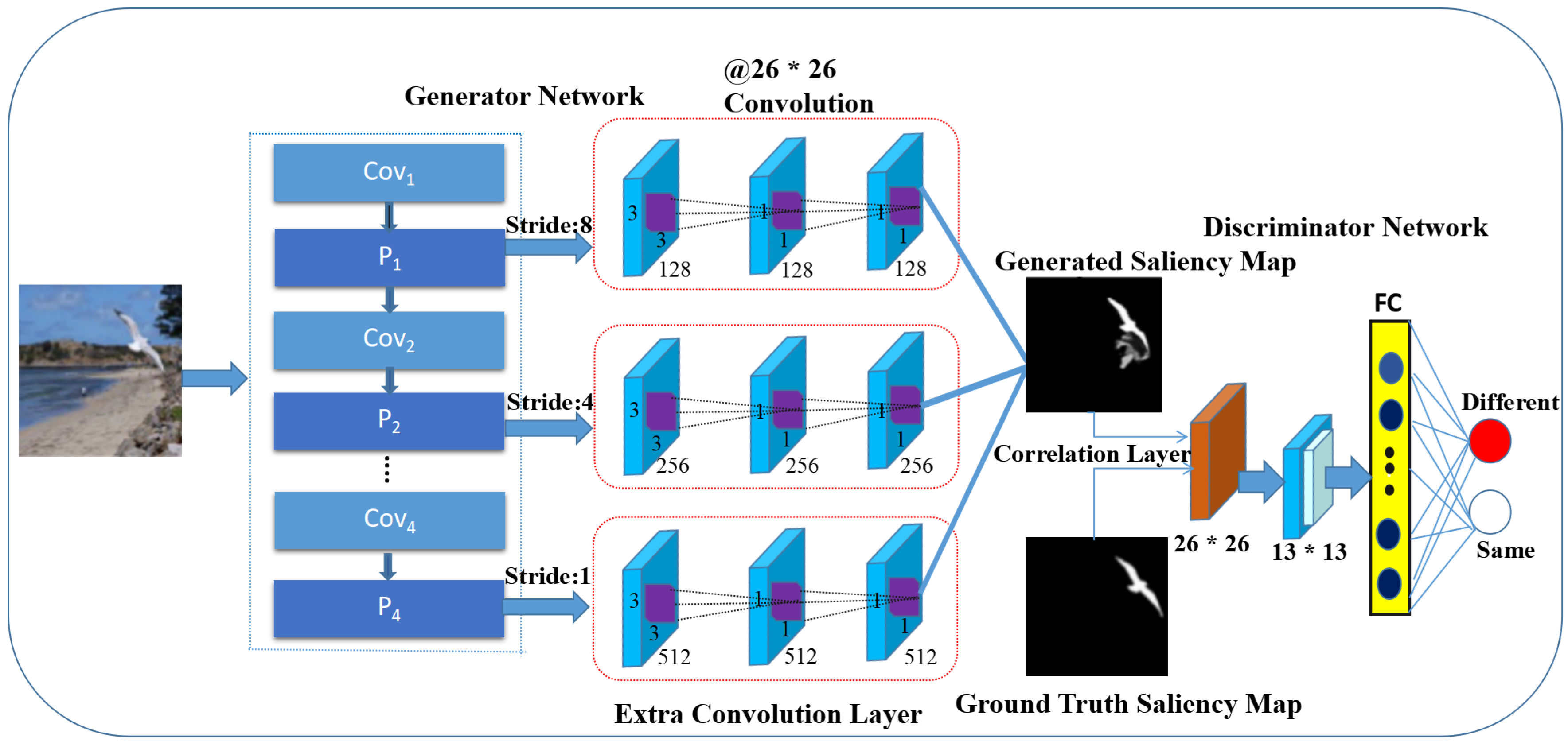
Different from previous work on saliency detection, we propose a new model named “multi-scale adversarial feature learning” (MAFL), which is built upon DCGAN (deep convolutional generative adversarial networks). We construct this model with the following considerations. At first, inspired by the strong ability of the adversarial features learned by GAN for image description, the adversarial features that are also devoted to image saliency are learned, and the synthesized image of the trained G-network becomes the target saliency map. That is to say, the aim of the traditional GAN model is to synthesize natural images, while our proposed MAFL model generates synthesized saliency maps. Secondly, considering that the scale problem is one of the most important cues that affects image saliency detection, we adjust the network structure of the G-network to make it compatible with the saliency detection task. Specifically, for each input image, different from the traditional G-network from which only the features from the top-level are output, the specially designed multi-scale G-network extracts features at multiple levels. Moreover, in order to capture subtle visual contrast on feature maps at each level, three extra convolution layers at each level of the G-network are successively added and performed to extract multi-scale deep contrast features. After obtaining deep contrast features at multiple scales for the input image, we fuse them as one feature vector, and the saliency map is obtained by passing the last soft-max layer. Thirdly, in order to enhance the discrimination ability, we apply a novel layer called the correlation layer to the D-network to discriminate the synthetic saliency map and the ground-truth saliency map accurately to the pixel-level. The detailed architecture of the proposed MAFL method is shown in Figure 1 and illustrated in Section 3.
To sum up, the main works we have done are as follows:
- We present a new multi-scale adversarial feature learning (MAFL) model based on the GAN model for image saliency detection. Instead of generating natural images, our MAFL model can directly obtain the image saliency map via the procedure of saliency map synthesis.
- We specially design a multi-scale G-network from which multiple scales of deep contrast features are extracted to incorporate the scale cue in image saliency detection.
- We provide a novel correlation layer in the D-network, by which the similarity between the synthetic saliency maps and the ground-truth saliency maps is calculated with the matching accuracy up to the per-pixel level.
The contents of each part of our paper are as follows. In Section 2, we analyze and discuss the traditional feature extraction methods and the CNN-based feature extraction methods for saliency detection. We describe the proposed MAFL model in detail in Section 3. In the next section, we make quantitative and qualitative comparisons on several public datasets, and compare our method to the other ten methods. Finally, we summarize the work and give our conclusion.
2. Related Work
We focus on analyzing and discussing the traditional feature extraction methods and the CNN-based feature extraction methods in the saliency detection.
Hand-crafted features: Most of the research work in saliency detection has been devoted to exploiting discriminative features [26,27,28,29,30,31]. Traditional hand-crafted features were the first type of features used. Thus, Itti et al. [32] first performed multi-channel feature extraction and then used the center-surround difference calculation to get feature maps on each feature dimension, followed by fusing these feature maps to obtain the aggregated saliency map. In [33], the author proposed a saliency detection method based on the frequency tuned for computing the saliency value of each pixel in an image. Ma et al. [34] employed color feature extraction in the local region of the image for image saliency estimation. Cheng et al. [6] proposed a method for extracting the color and region feature of an image to perform saliency detection. In [13], the author proposed a saliency measure based on feature uniqueness and spatial consistency. Jiang et al. [28] proposed to directly map region feature vectors to saliency values. Liu et al. [11] performed saliency detection by extracting local and global level features and using the conditional random field (CRF) to fuse these features. Although significant advances have been made, there are some pressing problems, especially when extracting hand-crafted features and performing heuristic fusion to obtain the final feature map. Firstly, the above-mentioned methods cannot detect targets in images with a cluttered background by extracting hand-crafted features. Secondly, these methods cannot detect salient objects with homogeneous highlight regions and accurate boundary information.
CNN-based deep features: Due to the wide application of artificial intelligence and deep learning techniques, a series of CNN-based saliency detection algorithms has appeared in the field of computer vision and significantly improved their performance. For example, Li et al. [14] presented a CNN-based saliency detection method to perform saliency detection by extracting multi-scale features. Zhao et al. [19] proposed a multi-task saliency detection method based on deep CNN, which performed saliency detection by extracting the semantic features of the object. Lee et al. [17] built a complete saliency detection model based on multiple CNN streams to extract multi-level features of the image. In [16], the authors provided a new method based on two CNN streams to extract features of local and global levels to perform saliency detection. In [35], the authors improved the traditional method by using the CNN framework to learn semantic features. Pan et al. [25] established a GAN-based supervised adversarial network model, which used the features of GAN to deal with image saliency detection. In our paper, we present a new multi-scale adversarial feature learning (MAFL) model for image saliency detection. In particular, we build this model, which is composed of two CNN modules: the multi-scale G-network takes natural images as inputs and generates the corresponding synthetic saliency map, and we design a novel layer in the D-network, namely a correlation layer, which is used to determine whether one image is a synthetic saliency map or ground-truth saliency map. Through experimental comparisons, we found that the performance of our approach has been greatly improved.
3. Our MAFL Model
Next, we focus on the structure and principle of the proposed MAFL model. Figure 1 shows the framework of our method. We proposed the saliency detection model, which consists of two deep neural networks, namely the generator network and the discriminator network, respectively. The multi-scale G-network takes natural images as inputs and generates the corresponding synthetic saliency map. In the D-network, we design a novel layer, namely a correlation layer, which is used to determine whether one image is a synthetic saliency map or a ground-truth saliency map. In this section, we will introduce them as follows.
3.1. Multi-Scale Generator Network
In our proposed MAFL model, we aim to design a multi-scale CNN to extract features that are discriminative enough to generate a realistic saliency map. We construct an end-to-end model with two considerations: (1) The designed network needs to be deep enough to generate a realistic saliency map. (2) The network is able to detect subtle visual contrast in the feature map at each level.
Compared with the GAN model, MAFL has a different structure for the G-network. The purpose of our design is to enable the GAN network to meet the task of image saliency detection. Some of our improvements to the G-network are mainly reflected in several aspects. Firstly, our proposed MAFL network consists of four pooling layers. For simplicity, the first two convolutional layers are tied together as , and we call each of the pooling layers a level. Since from the first level to the last level, the receptive field is expanded gradually, feature maps generated at each level correspond to features at different scales. Thus, feature maps at all levels are used for fusion of the final saliency map (synthetic saliency map).
Secondly, in order to find more subtle visual contrast in the extracted features at each level, we add an extra three convolution layers after each of the first four max-pooling layers in the MAFL network. By expanding the receptive field of these feature maps, we expect to obtain more subtle features of the natural image. The layers of the parameters in the network are shown in Figure 2. However, after three extra layers of convolutions, the feature maps obtained at each level have different sizes. In order to make them have the same size, we set the step size of the first extra layer added at each level to 8, 4, 2 and 1, respectively. In this way, we obtain four scales of feature maps with subtle visual contrast refined. An example of features learned at different layers is shown in Figure 3. Figure 3a shows the original image, and Figure 3b describes the convolution features learned in the first layer, such as color, contrast, corner and edge features. Figure 3c,d present the output of the 3th and 4th layers, respectively. From these two figures, it can be seen that the salient parts in the feature maps at different levels are highlighted.
At last, in order to enhance the effect of feature learning, we fuse the feature maps at four scales. Then, the fused result is sent into a final convolution layer with a convolution kernel, one channel. The convolution is actually performed as a fusion step, and the result after convolution is our multi-scale deep feature map (synthetic saliency map) of the input natural image. Experiments demonstrate that our model and configuration can significantly enhance the stability and improve its performance.
3.2. Discriminator Network
In general, the D-network in the MAFL model has a similar structure as its counterpart in GAN. However, compared with GAN model, MAFL introduces a novel layer to further improve the saliency detection performance, i.e., correlation layer. In the D-network, we assume that the input is a ground-truth saliency map and its corresponding synthetic saliency map. During the forward procedure, we measure the similarity between the two saliency maps via a correlation layer. Here, denote two saliency maps and as the ground-truth saliency map and synthetic saliency map, respectively. The correlation layer is to compare each patch in with each patch in , where is the patch size. Mathematically, for each location in , we compute correlation only in the neighborhood of centered at , and the size of the neighborhood is set to , where represents the maximum displacement. The formulation comes to:
Note that in Equation (1), different from general convolution, which is convolving data with a filter, we convolve data with other data. It is also worth mentioning that if this network is large enough, the similarity of two saliency map can be calculated accurately to the pixel-wise level. In this way, we obtain the similarity of two saliency maps. If the C value is large enough, it means that the synthetic saliency map generated by the G-network is more realistic. Meanwhile, it can also show that our proposed model is superior to other methods in performance.
4. Experiments
In this section, we validate our proposed MAFL method through experimental results. We first perform comparisons between the different methods on several benchmark datasets. Secondly, in order to further demonstrate the advantages of adding multi-scale GAN in the MAFL model, we perform comparisons by using single GAN. Finally, we replace the GAN network in the MAFL framework with a different network architecture, which demonstrates the advantages of using GAN in our model.
4.1. Dataset
In our proposed method, three public datasets are used to perform experiments.
THUR15K [36]: This dataset contains 6232 images and consists of five object categories. This dataset is unique because some of images contained in it do not have salient target.
PASCAL-S [37]: The dataset is derived from the PASCAL VOC2010 segmentation challenge dataset, which contains 850 images with multiple targets and a complex background.
4.2. Evaluation Criteria
To reflect the fairness of the comparison between the methods, we used three common evaluation criteria.
Precision-recall curve: Because the ROC [38] does not provide sufficient evaluation information, we use the P-R [12] curve for method comparison.
The process of obtaining the P-R curve is as follows: for a saliency map, we first binarize it using a threshold to obtain the corresponding binary mark (B); then compare the binary mask (B) with the corresponding ground-truth (G); finally, calculate the average precision and recall value in the whole dataset. The formula is as follows:
F-measure: When evaluating some methods, sometimes using the P-R curve does not really reflect the performance of the method. Therefore, we use the F-measure to comprehensively evaluate the methods. The formula for calculating the F-measure is as follows:
According to empirical evidence, we set to 0.3.
MAE: We use MAE (mean absolute error) to reduce the average error of TPR (true positive rate) and TNR (true negative rate), which can fit the relations between them. and denote the saliency map and ground-truth at the pixel , respectively. Therefore, the formula for calculating MAE is as follows:
4.3. Comparisons with Different Methods
In order to demonstrate the effectiveness of the proposed method, we compare our method with different methods on three benchmark datasets. We trained our proposed method on the THUR15K dataset, which contains 6232 images. To reflect the rationality of the training, we choose 5000 images for training and 1232 images for testing. We compare the proposed method with ten state-of-the-art approaches, including UCF [39], DCL [18], DS [19], KSR [40], SRM [41], NLDF [42], RST [43], ELD [17], SMD [44] and WSS [45]. In order to highlight significantly the advantages of our approach, we have made qualitative and quantitative comparisons of these methods.
Quantitative comparison: Figure 4 shows the visualization of the saliency maps obtained by our method and ten different methods. We can see from Figure 4 that our method can not only uniformly highlight the whole salient objects, but also preserves the details of the objects’ structure. Experiments on several datasets show that our method can produce excellent results in a variety of complex and challenging images. For example, there is a lower contrast between the target and background (Row 5); the image contains a cluttered background (Row 3); the image contains multiple salient objects (Rows 1, 2 and 5); and the objects are close to the border of the image (Row 4).
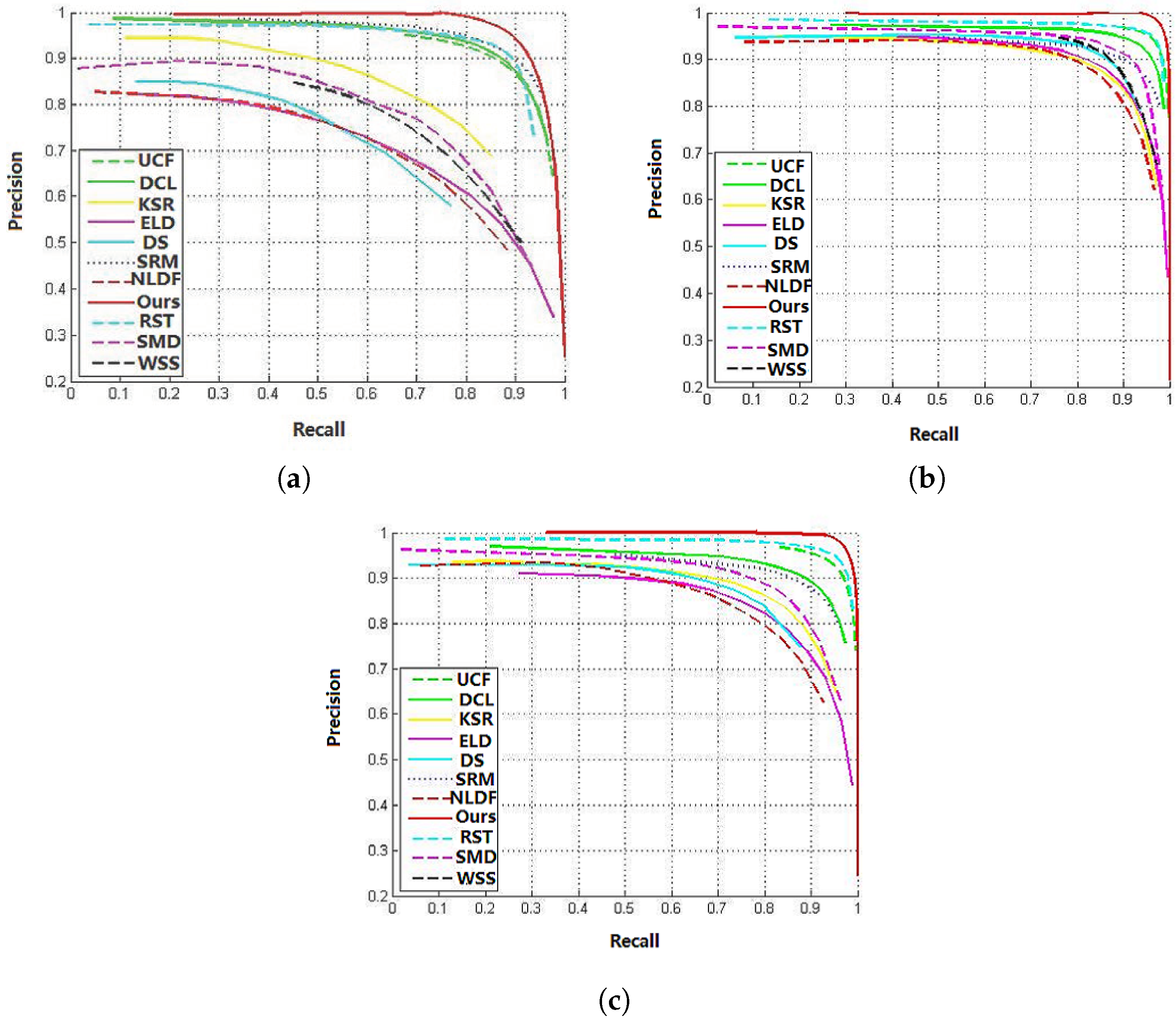
Qualitative comparison: We use the P-R curves to compare our method with the other ten methods. As can be seen from Figure 5, compared to the other ten approaches, our approach obtains the highest P-R curve on three benchmark datasets. The best performance is on the THUR15K dataset: our method achieves a precision value of 94.46%, which is better than the current best method (the precision value of the RST method is 92.54%) of 1.2%. Meanwhile, our method also achieves a 98.59% recall value, which significantly outperforms other methods.
At the same time, we also compare the proposed approach with other approaches using F-measure values on the datasets. Figure 6 shows the comparison of the different methods. It can be seen from Figure 6 that our approach obtains the highest F-measure value, which is significantly higher than other methods. Especially on the MSRA-A dataset, our method’s F-measure value increases from 0.862 to 0.8948 compared to the current best method (RST). On the THUR15K and PASCAL-S datasets, the F-measure of our proposed approach has also been greatly enhanced.
In order to further evaluate the generated synthetic saliency map, we use MAE as the evaluation metric, and Figure 7 shows the MAE values on the three datasets. We can see from Figure 7 that our method has achieved the smallest MAE value on all datasets. Compared with the current best performance approach (RST), our approach outperforms it. Especially on the PASCAL-S dataset, our method obtained the highest MAE value and successfully reduced the MAE value by 3.03%. Therefore, we can prove the effectiveness of the proposed method by this evaluation metric.
4.4. Performance Comparisons of Our MAFL Model with Multi-Scale and Single-Scale
To better show the superiority of the MAFL method with multi-scale feature extraction, comparisons are performed for our MAFL model with multi-scale GAN (MGAN) and single-scale GAN (SGAN). In our paper, MAFL with MGAN is our proposed model with four levels of output features, while the MAFL model with SGAN with only one level. Except for the different network architectures, all other settings of the two models are kept untouched. In this way, we can compare the experimental results of scale differences. We perform the experiment on the MAFL model with the MGAN configuration and the MAFL model with the SGAN configuration, respectively. Figure 8 shows the experimental results. We can see from Figure 8 that the result by using designed MAFL model with MGAN configuration is significantly better than MAFL with SGAN configuration.
4.5. Comparison of Experimental Results with Other Neural Networks
To further demonstrate the effectiveness of the proposed model with GAN, we replaced GAN in our MAFL architecture with other deep neural networks: GoogleNet, AlexNet and CNN. To further show the fairness of comparison, we compared MAFL model with different network structures on one dataset (MSRA-A). Except for the difference of the network architectures, other settings were kept the same. Figure 9 and Table 1 show that the MAFL model with multi-scale GAN performed significantly better than MAFL model with GoogleNet and AlexNet. In summary, by comparing the deep neural network models, we can see that the MAFL method had the advantage of GAN.
4.6. Comparison of Execution Time
In this subsection, in order to compare the advantages and disadvantages of each method more intuitively and clearly, we introduce another evaluation metric, that is the comparison of the execution time. By studying the performance of other methods, we found that many methods often achieve superior performance at the expense of time. However, our proposed method not only achieved excellent performance, it also had the shortest execution time. The execution times of different methods are shown in Table 2. From this table, we can see that our method achieves the shortest execution time.
5. Conclusions
In our paper, we propose a novel multi-scale adversarial feature learning (MAFL) approach for image saliency detection. The proposed saliency detection model consists of two CNN networks, which are the multi-scale generator network and the discriminator network. Firstly, we define a multi-scale G-network, which takes original images as inputs and generates corresponding synthetic saliency maps. Secondly, we design a novel layer in the D-network, namely a correlation layer, to compare the similarity between the synthetic saliency map and ground-truth saliency map. We further demonstrate that adversarial feature learning can significantly improve the performance. Experimental results on several public benchmark datasets demonstrate that the proposed method outperforms other existing methods.
Author Contributions
D.Z. and L.D. conceived of and designed the experiments. Y.L. and X.S. analyzed the data. J.L., G.Z. and L.I. contributed analysis tools.
Funding
This work was supported in part by the General Program of the National Natural Science Foundation of China (NSFC) under Grant No.61572362, in part by the NSFC under Grant No. 81571347 and in part by the Fundamental Research Funds for the Central Universities under Grant No. 22120180012.
Acknowledgments
The authors are grateful for the comments and reviews from the reviewers and editors.
Conflicts of Interest
The authors declare no conflict of interest.
References
- Kuznetsova, P.; Ordonez, V.; Berg, A.; Berg, T. Generalizing Image Captions for Image-Text Parallel Corpus. In Proceedings of the Meeting of the Association for Computational Linguistics, Sofia, Bulgaria, 4–9 August 2013; pp. 790–796. [Google Scholar]
- Marat, S.; Guironnet, M.; Pellerin, D. Video summarization using a visual attention model. In Proceedings of the Signal Processing Conference, Poznan, Poland, 3–7 September 2007; IEEE: Piscataway, NJ, USA, 2015; pp. 1784–1788. [Google Scholar]
- Lv, X.; Zou, D.; Zhang, L.; Jia, S. Feature coding for image classification based on saliency detection and fuzzy reasoning and its application in elevator videos. WSEAS Trans. Comput. 2014, 13, 266–276. [Google Scholar]
- Wu, L.; Shen, C.; Hengel, A.V.D. PersonNet: Person Re-identification with Deep Convolutional Neural Networks. In Proceedings of the Computer Vision and Pattern Recognition, Las Vegas Valley, NV, USA, 26 June–1 July 2016; pp. 3908–3915. [Google Scholar]
- Ren, Z.; Gao, S.; Chia, L.-T.; Tsang, I.W.-H. Region-Based Saliency Detection and Its Application in Object Recognition. IEEE Trans. Circuits Syst. Video Technol. 2014, 24, 769–779. [Google Scholar] [CrossRef]
- Cheng, M.-M.; Mitra, N.J.; Huang, X.; Torr, P.H.S.; Hu, S.-M. Global contrast based salient region detection. In Proceedings of the Computer Vision and Pattern Recognition, Colorado Springs, CO, USA, 20–25 June 2011; IEEE: Washington, DC, USA, 2011; pp. 409–416. [Google Scholar]
- Itti, L.; Koch, C. Comparison of feature combination strategies for saliency-based visual attention systems. In Proceedings of the SPIE—The International Society for Optical Engineering, San Jose, CA, USA, 23–29 January 1999; Volume 3644, pp. 473–482. [Google Scholar]
- Borji, A.; Cheng, M.M.; Hou, Q.; Jiang, H.; Li, J. Salient Object Detection: A Survey. arxiv, 2014; arXiv:1411.5878. [Google Scholar]
- Tamrakar, A.; Ali, S.; Yu, Q.; Liu, J.; Javed, O.; Divakaran, A.; Cheng, H. Evaluation of low-level features and their combinations for complex event detection in open source videos. In Proceedings of the IEEE Conference on Computer Vision and Pattern Recognition, Providence, RI, USA, 16–21 June 2012; IEEE Computer Society: Washington, DC, USA, 2012; pp. 3681–3688. [Google Scholar]
- Qi, W.; Cheng, M.-M.; Borji, A.; Lu, H.; Bai, L.-F. SaliencyRank: Two-stage manifold ranking for salient object detection. Comput. Vis. Media 2015, 1, 309–320. [Google Scholar] [CrossRef]
- Liu, T.; Yuan, Z.; Sun, J.; Zheng, N.-N.; Tang, X.; Shum, H.-Y. Learning to Detect a Salient Object. IEEE Trans. Pattern Anal. Mach. Intell. 2010, 33, 353–367. [Google Scholar]
- Yang, C.; Zhang, L.; Lu, H.; Ruan, X.; Yang, M.-H. Saliency Detection via Graph-Based Manifold Ranking. In Proceedings of the Computer Vision and Pattern Recognition, Portland, OR, USA, 23–28 June 2013; IEEE: Piscataway, NJ, USA, 2013; pp. 3166–3173. [Google Scholar] [Green Version]
- Krahenbuhl, P. Saliency filters: Contrast based filtering for salient region detection. In Proceedings of the 2012 IEEE Conference on Computer Vision and Pattern Recognition, Providence, RI, USA, 16–21 June 2012; IEEE Computer Society: Washington, DC, USA, 2012; pp. 733–740. [Google Scholar] [Green Version]
- Li, G.; Yu, Y. Visual saliency based on multiscale deep features. In Proceedings of the Computer Vision and Pattern Recognition, Boston, MA, USA, 7–12 June 2015; IEEE: Piscataway, NJ, USA, 2015; pp. 5455–5463. [Google Scholar] [Green Version]
- Chen, T.; Lin, L.; Liu, L.; Luo, X.; Li, X. DISC: Deep Image Saliency Computing via Progressive Representation Learning. IEEE Trans. Neural Netw. Learn. Syst. 2016, 27, 1135. [Google Scholar] [CrossRef] [PubMed]
- Wang, L.; Lu, H.; Ruan, X.; Yang, M.-H. Deep networks for saliency detection via local estimation and global search. In Proceedings of the IEEE Conference on Computer Vision and Pattern Recognition, Boston, MA, USA, 7–12 June 2015; pp. 3183–3192. [Google Scholar]
- Lee, G.; Tai, Y.W.; Kim, J. Deep Saliency with Encoded Low Level Distance Map and High Level Features. In Proceedings of the IEEE Conference on Computer Vision and Pattern Recognition, Las Vegas, NV, USA, 27–30 June 2016; pp. 660–668. [Google Scholar]
- Li, G.; Yu, Y. Deep contrast learning for salient object detection. In Proceedings of the IEEE Conference on Computer Vision and Pattern Recognition, Las Vegas, NV, USA, 27–30 June 2016; pp. 478–487. [Google Scholar]
- Li, X.; Zhao, L.; Wei, L.; Yang, M.-H.; Wu, F.; Zhuang, Y.; Ling, H.; Wang, J. Deepsaliency: Multi-task deep neural network model for salient object detection. IEEE Trans. Image Process. 2016, 25, 3919–3930. [Google Scholar] [CrossRef] [PubMed]
- Hou, Q.; Cheng, M.-M.; Hu, X.-W.; Borji, A.; Tu, Z.; Torr, P. Deeply supervised salient object detection with short connections. In Proceedings of the 2017 IEEE Conference on Computer Vision and Pattern Recognition (CVPR), Honolulu, HI, USA, 21–26 July 2017; IEEE: Piscataway, NJ, USA, 2017; pp. 5300–5309. [Google Scholar]
- Goodfellow, I.J.; Pouget-Abadie, J.; Mirza, M.; Xu, B.; Warde-Farley, D.; Ozair, S.; Courville, A.; Bengio, Y. Generative adversarial nets. In Proceedings of the International Conference on Neural Information Processing Systems, Montreal, QC, Canada, 8–13 December 2014; MIT Press: Cambridge, MA, USA, 2014; pp. 2672–2680. [Google Scholar]
- Luc, P.; Couprie, C.; Chintala, S.; Verbeek, J. Semantic Segmentation using Adversarial Networks. In Proceedings of the NIPS Workshop on Adversarial Training, Barcelona, Spain, 9 December 2016. [Google Scholar]
- Li, J.; Liang, X.; Wei, Y.; Xu, T.; Feng, J.; Yan, S. Perceptual Generative Adversarial Networks for Small Object Detection. In Proceedings of the 2017 IEEE Conference on Computer Vision and Pattern Recognition (CVPR), Honolulu, HI, USA, 21–26 July 2017; pp. 1951–1959. [Google Scholar]
- Cai, X.; Yu, H. Saliency detection by conditional generative adversarial network. In Proceedings of the Ninth International Conference on Graphic and Image Processing (ICGIP 2017), Qingdao, China, 14–16 October 2017; International Society for Optics and Photonics: Bellingham, WA, USA, 2018; Volume 10615. [Google Scholar]
- Pan, H.; Jiang, H. Supervised Adversarial Networks for Image Saliency Detection. arXiv, 2017; arXiv:1704.07242. [Google Scholar]
- Tang, Y.; Wu, X. Saliency Detection via Combining Region-Level and Pixel-Level Predictions with CNNs; Springer: New York, NY, USA, 2016; pp. 809–825. [Google Scholar]
- Borji, A. Exploiting Local and Global Patch Rarities for Saliency Detection. In Proceedings of the 2012 IEEE Conference on Computer Vision and Pattern Recognition, Providence, RI, USA, 16–21 June 2012; IEEE: Piscataway, NJ, USA, 2012; pp. 478–485. [Google Scholar]
- Jiang, H.; Wang, J.; Yuan, Z.; Wu, Y.; Zheng, N.; Li, S. Salient Object Detection: A Discriminative Regional Feature Integration Approach. In Proceedings of the 2013 IEEE Conference on Computer Vision and Pattern Recognition, Portland, OR, USA, 23–28 June 2013; IEEE Computer Society: Washington, DC, USA, 2013; pp. 2083–2090. [Google Scholar]
- Tong, N.; Lu, H.; Xiang, R.; Yang, M.-H. Salient object detection via bootstrap learning. In Proceedings of the 2015 IEEE Conference on Computer Vision and Pattern Recognition, Boston, MA, USA, 7–12 June 2015; IEEE: Piscataway, NJ, USA, 2015; pp. 1884–1892. [Google Scholar]
- Tong, N.; Lu, H.; Zhang, Y.; Ruan, X. Salient object detection via global and local cues. Pattern Recognit. 2015, 48, 3258–3267. [Google Scholar] [CrossRef]
- Wang, J.; Lu, H.; Li, X.; Tong, N.; Liu, W. Saliency detection via background and foreground seed selection. Neurocomputing 2015, 152, 359–368. [Google Scholar] [CrossRef]
- Itti, L.; Koch, C.; Niebur, E. A Model of Saliency-Based Visual Attention for Rapid Scene Analysis. IEEE Trans. Pattern Anal. Mach. Intell. 1998, 20, 1254–1259. [Google Scholar] [CrossRef]
- Achanta, R.; Hemami, S.; Estrada, F.; Susstrunk, S. Frequency-tuned salient region detection. In Proceedings of the 2009 IEEE Conference on Computer Vision and Pattern Recognition, CVPR 2009, Miami, FL, USA, 20–25 June 2009; IEEE: Piscataway, NJ, USA, 2009; pp. 1597–1604. [Google Scholar] [Green Version]
- Ma, Y.F.; Zhang, H.J. Contrast-based image attention analysis by using fuzzy growing. In Proceedings of the Eleventh ACM International Conference on Multimedia, Berkeley, CA, USA, 2–8 November 2003; ACM: New York, NY, USA, 2003; pp. 374–381. [Google Scholar]
- Shen, C.; Zhao, Q. Learning to predict eye fixations for semantic contents using multi-layer sparse network. Neurocomputing 2014, 138, 61–68. [Google Scholar] [CrossRef]
- Cheng, M.-M.; Mitra, N.J.; Huang, X.; Hu, S.-M. SalientShape: Group Saliency in Image Collections. Available online: http://mmcheng.net/gsal/ (accessed on 1 October 2018).
- Li, Y.; Hou, X.; Koch, C.; Rehg, J.M.; Yuille, A.L. The Secrets of Salient Object Segmentation. In Proceedings of the 2014 IEEE Conference on Computer Vision and Pattern Recognition, Columbus, OH, USA, 23–28 June 2014; IEEE: Piscataway, NJ, USA, 2014; pp. 280–287. [Google Scholar] [Green Version]
- Goferman, S.; Zelnik-Manor, L.; Tal, A. Context-aware saliency detection. IEEE Trans. Pattern Anal. Mach. Intell. 2012, 34, 1915–1926. [Google Scholar] [CrossRef] [PubMed]
- Zhang, P.; Wang, D.; Lu, H.; Wang, H.; Yin, B. Learning uncertain convolutional features for accurate saliency detection. In Proceedings of the 2017 IEEE International Conference on Computer Vision (ICCV), Venice, Italy, 22–29 October 2017; IEEE: Piscataway, NJ, USA, 2017; pp. 212–221. [Google Scholar]
- Wang, T.; Zhang, L.; Lu, H.; Sun, C.; Qi, J. Kernelized subspace ranking for saliency detection. In Proceedings of the European Conference on Computer Vision, Amsterdam, The Netherlands, 11–14 October 2016; Springer: Cham, Switzerland, 2016; pp. 450–466. [Google Scholar]
- Wang, T.; Borji, A.; Zhang, L.; Zhang, P.; Lu, H. A stagewise refinement model for detecting salient objects in images. In Proceedings of the IEEE International Conference on Computer Vision, Venice, Italy, 22–29 October 2017; pp. 4019–4028. [Google Scholar]
- Luo, Z.; Mishra, A.; Achkar, A.; Eichel, J.; Li, S.; Jodoin, P.-M. Non-local deep features for salient object detection. In Proceedings of the 2017 IEEE Conference on Computer Vision and Pattern Recognition, Honolulu, HI, USA, 21–26 July 2017. [Google Scholar]
- Zhu, L.; Ling, H.; Wu, J.; Deng, H.; Liu, J. Saliency Pattern Detection by Ranking Structured Trees. In Proceedings of the IEEE International Conference on Computer Vision, Venice, Italy, 22–29 October 2017; pp. 5467–5476. [Google Scholar]
- Peng, H.; Li, B.; Ling, H.; Hu, W.; Xiong, W.; Maybank, S.J. Salient object detection via structured matrix decomposition. IEEE Trans. Pattern Anal. Mach. Intell. 2016, 99, 1–14. [Google Scholar] [CrossRef] [PubMed]
- Wang, L.; Lu, H.; Wang, Y.; Feng, M.; Wang, D.; Yin, B.; Ruan, X. Learning to detect salient objects with image-level supervision. In Proceedings of the 2017 IEEE Conference on Computer Vision and Pattern Recognition (CVPR), Honolulu, HI, USA, 21–26 July 2017; pp. 136–145. [Google Scholar]
Figure 1.
The overview of our proposed multi-scale adversarial feature learning model. It should be noted that is the tied convolution layer, is the max-pooling layer and FC represents the fully-connected layer.
Figure 1.
The overview of our proposed multi-scale adversarial feature learning model. It should be noted that is the tied convolution layer, is the max-pooling layer and FC represents the fully-connected layer.

Figure 2.
Layer parameters of the multi-scale adversarial feature learning (MAFL) model. FS: the size of the convolution kernel. The representation of the network layer: C: convolution, P: max pooling, Ex_P_C: add extra convolution layers to the first four max-pooling layers.
Figure 2.
Layer parameters of the multi-scale adversarial feature learning (MAFL) model. FS: the size of the convolution kernel. The representation of the network layer: C: convolution, P: max pooling, Ex_P_C: add extra convolution layers to the first four max-pooling layers.

Figure 3.
Visual representation of feature learning in the MAFL model on the PASCAL-Sdataset. (a) Input image; (b) features learned in the layer; (c) visualization of learned features at the layer; (d) visualization of learned features at the layer.
Figure 3.
Visual representation of feature learning in the MAFL model on the PASCAL-Sdataset. (a) Input image; (b) features learned in the layer; (c) visualization of learned features at the layer; (d) visualization of learned features at the layer.

Figure 4.
Visualization of the saliency maps obtained by our approach and other methods on the MSRA-A, PASCAL-S and THUR15Kdatasets. The saliency map generated by our method is shown in the second to last column, which is the best estimate of the ground-truth. Compare with other different approaches: UCF [39], DCL [18], DS [19], KSR [40], SRM [41], NLDF [42], RST [43], ELD [17], SMD [44] and WSS [45].

Figure 5.
Compare P-Rcurves for multiple approaches on several datasets: (a) MSRA-A dataset; (b) PASCAL-S dataset; (c) THUR15K dataset.
Figure 5.
Compare P-Rcurves for multiple approaches on several datasets: (a) MSRA-A dataset; (b) PASCAL-S dataset; (c) THUR15K dataset.

Figure 6.
Compare multiple approaches using F-measure values on several public datasets: (a) MSRA-A dataset; (b) PASCAL-S dataset; (c) THUR15K dataset.
Figure 6.
Compare multiple approaches using F-measure values on several public datasets: (a) MSRA-A dataset; (b) PASCAL-S dataset; (c) THUR15K dataset.


Figure 7.
Compare MAE values for multiple approaches on several datasets: (a) MSRA-A dataset; (b) PASCAL-S dataset; (c) THUR15K dataset.
Figure 7.
Compare MAE values for multiple approaches on several datasets: (a) MSRA-A dataset; (b) PASCAL-S dataset; (c) THUR15K dataset.

Figure 8.
Performance comparison on the MSRA-A dataset for the MAFL model with multi-scale and MAFL with single-scale, respectively. GAN, generative adversarial network.
Figure 8.
Performance comparison on the MSRA-A dataset for the MAFL model with multi-scale and MAFL with single-scale, respectively. GAN, generative adversarial network.

Figure 9.
Comparison with other neural network models on the MSRA-A dataset: (a) input image; (b) AlexNet; (c) GoogleNet; (d) ours.
Figure 9.
Comparison with other neural network models on the MSRA-A dataset: (a) input image; (b) AlexNet; (c) GoogleNet; (d) ours.


Table 1.
The F-measure values for the three deep neural networks on the MSRA-A dataset.
| Different Types of Neural Networks | F-Measure |
|---|---|
| 0.832 | |
| 0.685 | |
| 0.728 | |
| 0.736 |
Table 2.
Comparison of the execution time (s) of each image on the MSRA-A dataset.
| Method | UCF | DCL | DS | KSR | SRM | NLDF | RST | ELD | SMD | WSS | Ours |
|---|---|---|---|---|---|---|---|---|---|---|---|
| Times (s) | 0.528 | 0.223 | 0.356 | 0.254 | 0.351 | 0.306 | 0.258 | 0.183 | 0.278 | 0.285 | 0.135 |
© 2018 by the authors. Licensee MDPI, Basel, Switzerland. This article is an open access article distributed under the terms and conditions of the Creative Commons Attribution (CC BY) license (http://creativecommons.org/licenses/by/4.0/).
Share and Cite
MDPI and ACS Style
Zhu, D.; Dai, L.; Luo, Y.; Zhang, G.; Shao, X.; Itti, L.; Lu, J. Multi-Scale Adversarial Feature Learning for Saliency Detection. Symmetry 2018, 10, 457. https://doi.org/10.3390/sym10100457
AMA Style
Zhu D, Dai L, Luo Y, Zhang G, Shao X, Itti L, Lu J. Multi-Scale Adversarial Feature Learning for Saliency Detection. Symmetry. 2018; 10(10):457. https://doi.org/10.3390/sym10100457
Chicago/Turabian StyleZhu, Dandan, Lei Dai, Ye Luo, Guokai Zhang, Xuan Shao, Laurent Itti, and Jianwei Lu. 2018. "Multi-Scale Adversarial Feature Learning for Saliency Detection" Symmetry 10, no. 10: 457. https://doi.org/10.3390/sym10100457
Note that from the first issue of 2016, this journal uses article numbers instead of page numbers. See further details here.