1. Introduction
Graphs have been used, since their informal beginnings, as a model to represent complex networks, to describe different properties within them and to find solutions to diverse problems, such as optimal routes or the best location of resources. Formally, a finite graph is a pair , where V is a non-empty finite set, whose elements are called vertices, and is a set of unordered pairs of vertices called edges. If is an edge, we say that u and v are neighbors. The distance between two vertices u and v in a graph is the number of edges in a shortest path connecting them and it is denoted by . The open neighborhood of a vertex u in a graph G is and the closed neighborhood is . The degree of a vertex is the cardinality of its open neighborhood.
Domination-type properties in graphs, formally defined in the late 1950s [
1] and early 1960s [
2], are a good example of how these models can help to represent real world problems and to provide optimal solutions to them. A
dominating set in a graph
G is a vertex set
S such that every vertex not in
S has at least one neighbor in
S. This classical definition provides a model of resource location in a network, in such a way that every node of the network has access to such a resource. Once this model is formulated, it is an immediate question to find the best possible distribution, which results in the definition of the
domination number of a graph
G, which is the minimum cardinality of a dominating set of
G. An extensive compilation of results on this subject can be found in [
3], as well as some of its applications such as the planning of school bus routes, the design of computer communication networks, the location of broadcasting stations, social networks modeling and land surveying.
Following this classic pattern, a large number of variants have been defined, which pay attention to different aspects. For instance, k-domination requests at least k neighbors in S for the vertices not in the k-dominating set S and locating-domination asks for for every pair of vertices . Another interesting variation consists of considering dominating sets with additional properties, such as connectedness or independence. A vertex set is connected if every two vertices in it can be joined by a sequence of edges consisting of vertices in the set. This model is useful to distribute resources in a network that need to be connected to each other. The opposite point of view is independence. A vertex set is independent if no pair of vertices in it are neighbors. Independent dominating sets have been widely studied, as they provide a model of resource location in cases where such resources should be placed far away from each other.
The most precise way to dominate a graph is the so-called efficient domination. A vertex set
S is an
efficient dominating set [
4], or
perfect code [
5,
6], if
S is independent and every vertex not in
S has a unique neighbor in
S. The idea behind this definition is keeping the domination of each vertex to the minimum, so that vertices in
S are dominated just by themselves, and vertices not in
S are dominated just once by vertices in
S. Clearly, this definition provides a desirable form of domination, which becomes even more interesting with the repeatedly rediscovered result that ensures every efficient dominating set is a minimum dominating set [
3]. However, the main problem with efficient dominating sets is that their existence is not guaranteed in every graph. There are well-known graph families that have no efficient dominating sets and, in these cases, a number of relaxations of conditions are possible in order to obtain a dominating set as efficient as possible. In this paper, we focus on one of these relaxed forms, called
independent -sets and defined in [
7]. The lower level of requirement of these sets consists of allowing at most two neighbors in the set, for vertices not in it, while keeping independence. Although existence is not guaranteed either in this case, the lesser requirement leads one to think that the family of graphs that possess such sets is larger than in the case of efficient domination. The
independent -number of a graph
G was also defined in [
7] as the minimum cardinality of an independent
-set, if such sets exist in
G, and it is denoted by
. The following general relationship among the three mentioned domination parameters can easily be deduced from definitions. Every graph
G satisfies the first inequality, while the last one is true for graphs admitting an independent
-set.
Given two graphs,
G and
H, the
Cartesian product of them is the graph
with vertex set
and edge set defined as follows:
if and only if
,
or
,
. Cartesian product graphs play an interesting role in the domination-type properties, due in part to the well-known Vizing’s Conjecture [
8], which states
for every two graphs
G and
H. It was formulated in 1968 and is still open.
We study the particular case of
cylindrical networks , which are the Cartesian product of a cycle
and a path
, and our interest comes from the known fact that they have no efficient dominating set, except in one particular case [
9]. On the other hand, studying the existence of independent
-sets in cylinders was proposed as an open problem in [
7]. Unlike in the case of
grids , the Cartesian product of two paths, where the domination number is completely computed [
10], the domination number of the cylinder is unknown in the general case, while formulas for
have recently been obtained for
[
11] and
[
12]. This makes cylinders a graph family of interest for domination-type properties, in which there is still much to study.
The rest of the paper is organized as follows. In
Section 2, we prove that all cylinders have an independent
-set, except the single case of the Cartesian product of the cycle with 5 vertices and the path with 2 vertices, which has no such set. We use the symmetry of the cylindrical graphs to provide regular models of independent
-sets that, in addition, will give an upper bound for the independent
-number. We will also prove that this upper bound is indeed the exact value, in some small cases. In
Section 3, we present a modification of a dynamic programming algorithm, originally developed for computing the domination number of grids, to provide information about the independent
-number in cylinders of selected sizes. Depending on the size of the cylinder, this modified algorithm computes the exact value of the parameter or just an upper bound for it. In the latter case we combine these results with an appropriate lower bound, in order to obtain the desired exact value. Finally, in
Section 4 and
Section 5 we present and discuss the experimental results obtained with the above mentioned algorithm. All graphs that appear in this paper are finite, simple and undirected. For undefined general concepts of graph theory, we refer to [
13].
2. Dominating a Cylinder as Efficiently as Possible
We devote this section to studying the existence of independent -sets in cylinders of any size. As we mentioned before, a cylinder is the Cartesian product of a cycle with vertices and a path with vertices. We will not consider the smallest case because all vertices in a cycle have degree two, so that every independent dominating set is trivially an independent -set.
We present some regular patterns that provide independent -sets in every cylinder, except in the case , where no such sets exist. The key point of this graph family is the particular symmetry of cylinders, which allows one to replicate small pieces in order to cover the whole graph.
The interest in obtaining independent -sets in cylinders lies in the known fact that just a particular case of them have an efficient dominating set, as we recall in the following proposition.
Proposition 1. [9] The cylinder has an efficient dominating set if and only if and . We begin our study about the behaviour of independent -sets in cylinders proving that has no such sets. This will eventually be the unique case of a cylinder failing this property.
Proposition 2. The cylinder has no independent -set.
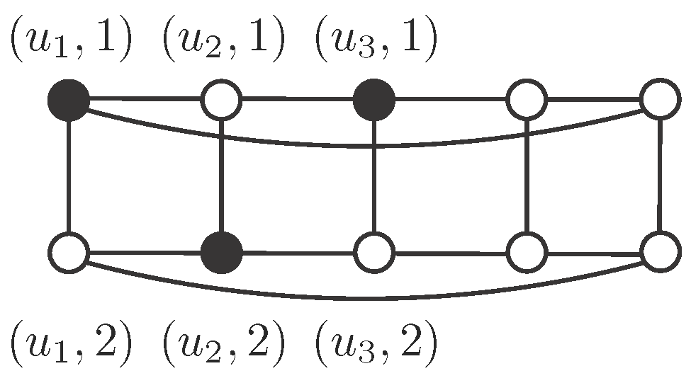
Proof. Denote by and suppose on the contrary that is an independent -set. Suppose that there exist at least two vertices in S sharing the second coordinate. By the symmetry of the graph, we may assume that .
Note that
, so it must be
, because
S is independent. By symmetry, we may assume that
and
. Then
, by independence, so
in order to be dominated. However, this means that
has three neighbors in
S, which is not possible (see
Figure 1). Therefore, if
then
for every
. In the same way, if
then
for every
. Finally,
, but
, a contradiction. □
We now focus on the rest of the cylinders with , where we provide an example of an independent -set in each size and we also obtain the exact value of the independent -number.
Proposition 3. Let be an integer. Then, the cylinder has an independent -set if and only if . Moreover, Proof. By Proposition 2, we know that
has no independent
-set. It is shown in [
14] that
, if
, and
, if
. For every integer
we will construct an independent
-set, with
vertices, so we will obtain that
.
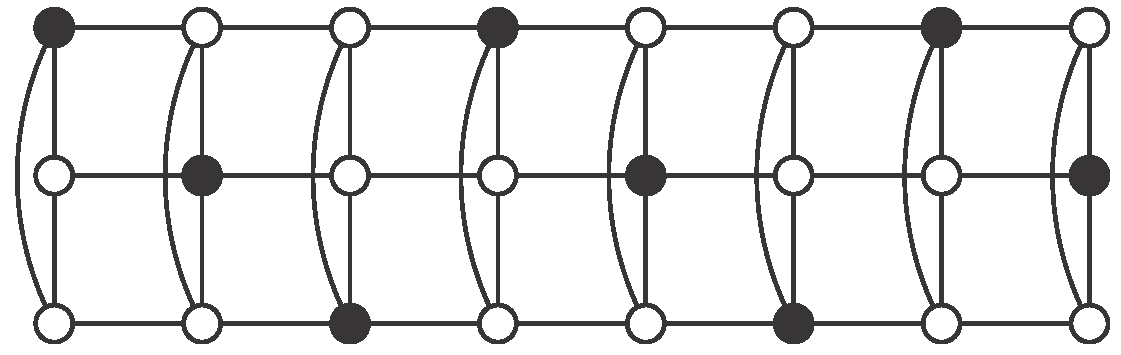
If
, then
and consider the set of black vertices in
Figure 2a. The basic block can be repeated
r times to obtain an independent
-set
S of
. Each basic block contains 2 vertices of
S, so
. Note that
S is also an efficient dominating set.
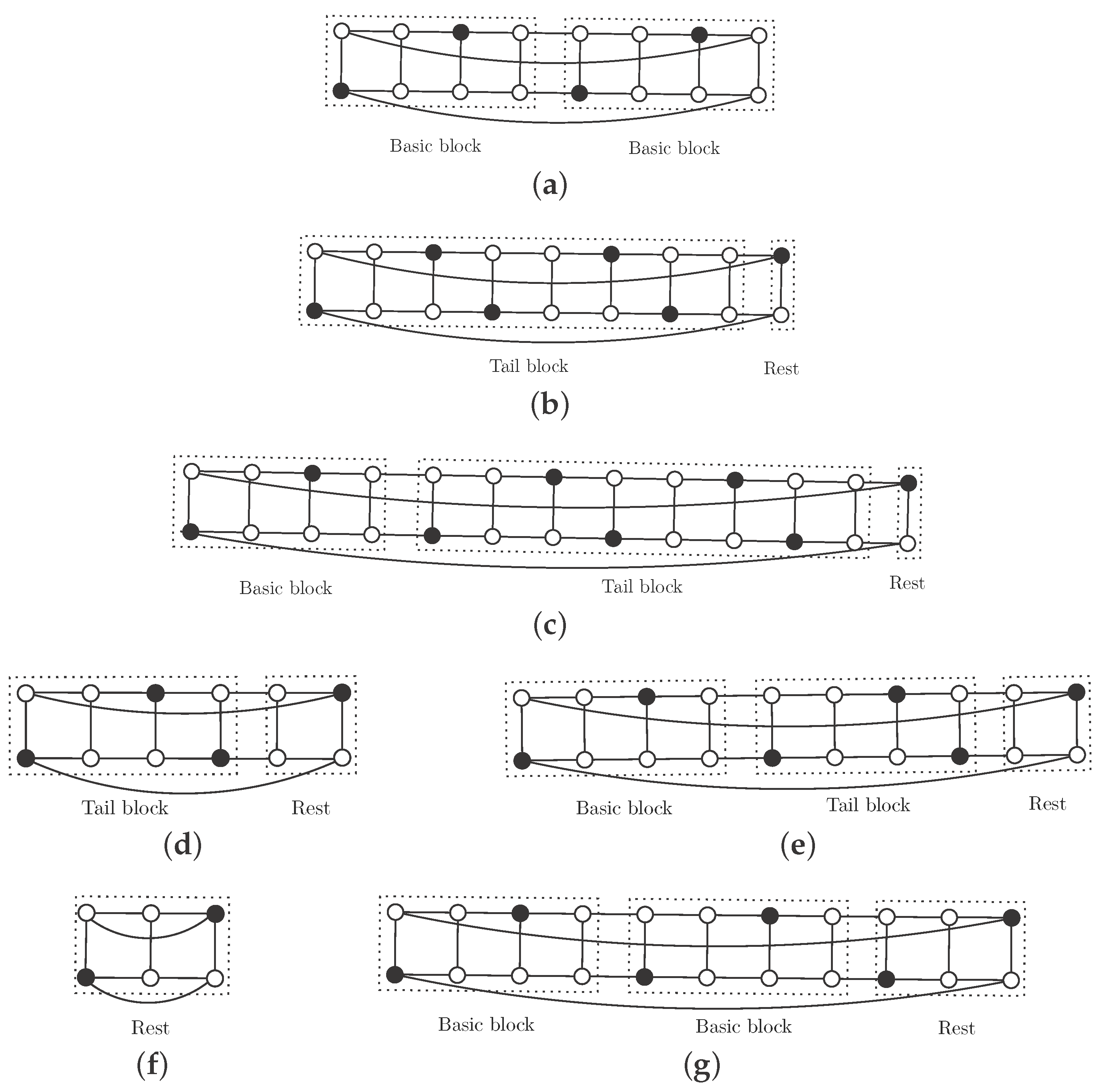
If
, then
and
. We repeat the basic block
times, add the tail block and the rest (see
Figure 2b for the case
and
Figure 2c for the general case
). We obtain an independent
-set
S (black vertices) with
vertices.
If
, then
and
. We add
copies of the basic block, the tail block for this case and the appropriate rest (see
Figure 2d for the case
and
Figure 2e for the general case
) and we obtain an independent
-set with
vertices.
If
, then
and
. We construct the independent
-set by adding
r copies of the basic block to the rest for this size, as is shown in
Figure 2f if
and in
Figure 2g if
. We obtain an independent
-set with
vertices.
Once we have proven the existence of an independent
-set in
(
), with size
, the desired equality now comes from Equation (
1). □
Remark 1. It is known that if and if [11]. In these cases, no efficient dominating set exists and Proposition 3 shows that minimum independent -sets play a similar role to such sets, in the sense that they provide the most efficient way of dominating these cylinders and they are at the same time minimum dominating sets. In the same way, we obtained the value of in the case n is as small as possible, we now study the case with the smallest cycle, that is . Here, we also supply an example of an independent -set that proves to be minimum. Henceforth, we will say that has m rows and n columns. Each row is a path with n vertices and each column is a cycle with m vertices. We numerate rows from top to bottom and we numerate columns from left to right.
Proposition 4. Let be an integer. Then the cylinder has an independent -set. Moreover, Proof. We just need to prove that
has an independent
-set with
elements. In
Figure 3, we show a regular pattern for such a set, for any value of
n. Clearly, this set has
n elements, one in each column, so
(for the last equality see [
14]). □
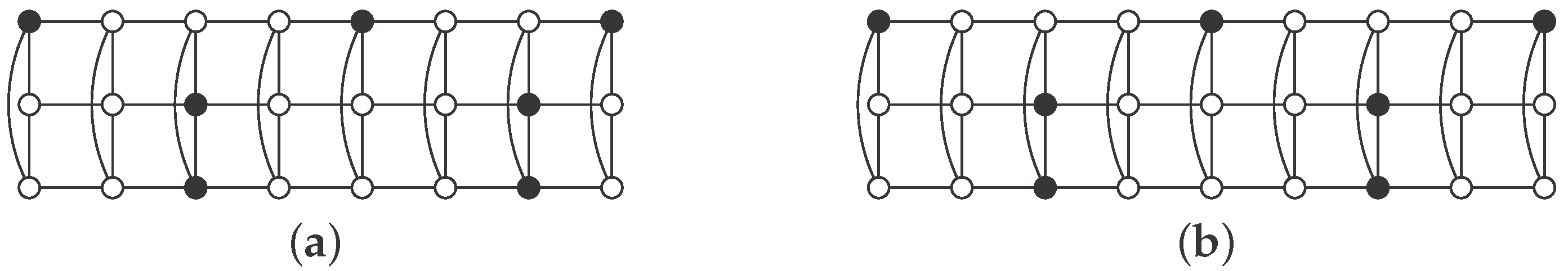
Remark 2. We would like to point out that the value of the domination number of cylinder that appears in [12], is not correct. The correct one is if and otherwise, and it can be found in [11]. In Figure 4a, we show a minimum dominating set of with vertices and, in Figure 4b, a dominating set of with vertices. None of them are independent sets; indeed, if and only if . Once we have studied the cases with the smallest values of m and n, we now focus on the general case. Our target is to prove that every cylinder , with and has an independent -set. To this end we construct regular patterns that can be replicated in order to cover all the cases. These patterns will also provide an upper bound of . We think that it could be possible to separately study some other small cases, for instance or , to obtain the exact values of the independent -number. However, we now prefer to provide general constructions, even if they are not minimum ones, that can be used in cylinders of any size, in order to prove the general existence of independent -sets. On the other hand, we will compute the exact value of for a number of small cases in the following sections. We divide our study into two results, one for odd paths and another for even paths. We begin with the odd case.
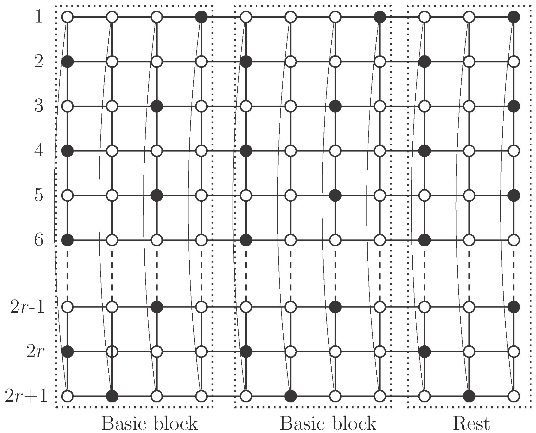
Theorem 1. Let be an integer and let be an odd integer. Then the cylinder has an independent -set. Moreover in this case Proof.
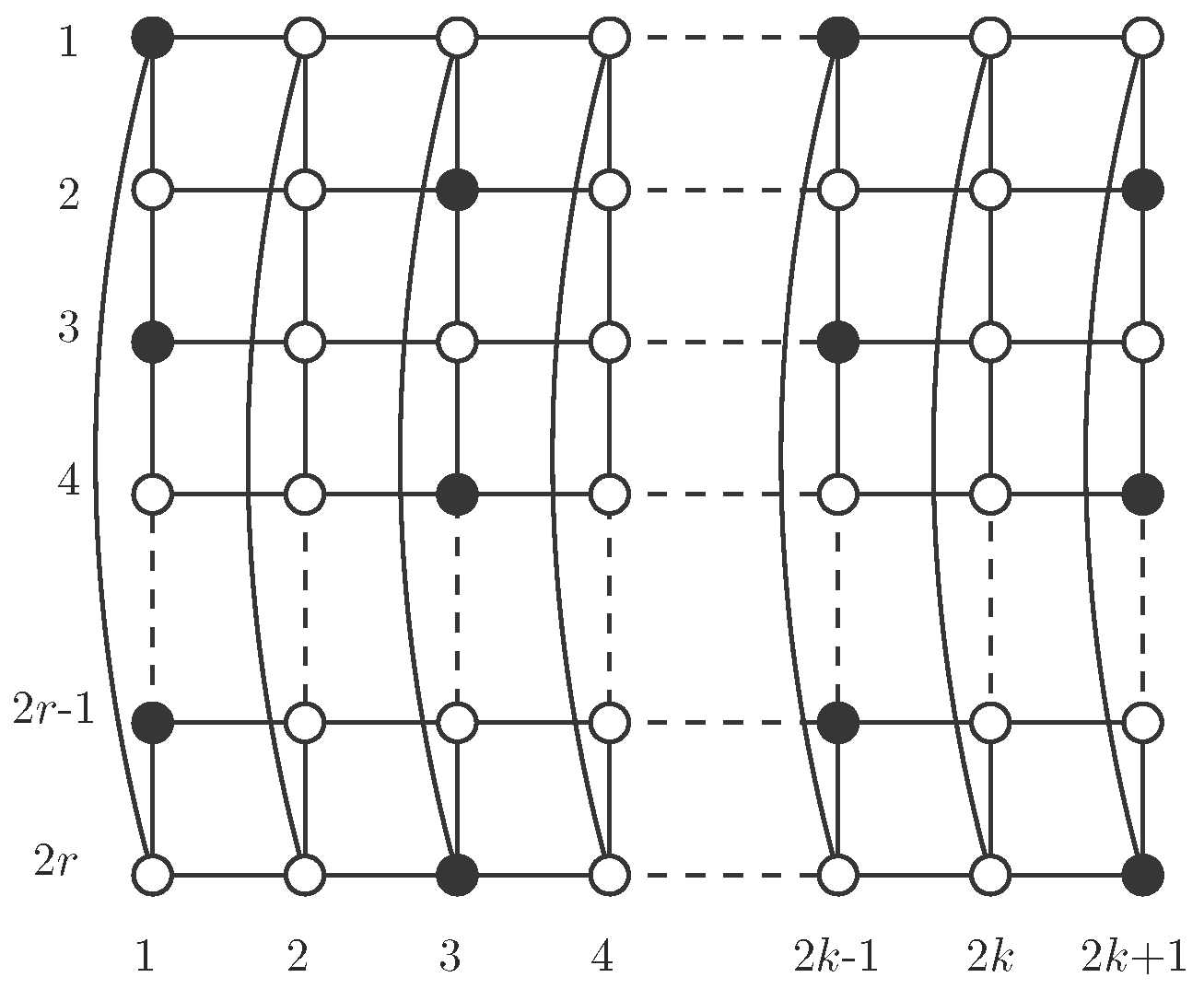
Case 1: .
Using
, consider the pattern described in
Figure 5, where set
S consists of black vertices. There are no vertices of
S in the even columns. Regarding odd columns, we begin with vertices in odd positions in the first one and then we alternate with vertices in even positions. Clearly
S is an independent
-set in
. Moreover, in each odd column there are
r vertices of
S, so
Case 2: and .
Consider the pattern described in
Figure 6. Here, we use a basic block with four columns, which we repeat
k times, and a rest with one column.
In the basic block, vertices in
S in the first column are in even positions, in the second column the unique vertex in
S is the last one. In the third column, vertices in
S are the ones in the odd positions, except the first and the last ones. Finally, in column number four, we pick just the first vertex. Therefore, there are
vertices of
S in each basic block (see
Figure 6).
The last column contains
r vertices in
S which are in even positions (see
Figure 6). Clearly,
S is an independent
-set of
and moreover,
Case 3: and .
We now take the pattern in
Figure 7. Again, we repeat the same basic block as before
k times, and we add a rest with three columns. If
and
, we just consider the rest with three columns. In any case, the resulting set
S is an independent
-set of
. We know that a basic block contains
vertices of
S and note that the rest contains
vertices of
S, therefore
We now complete the study of the existence of independent -sets in cylinders with the following theorem, covering the remaining case, that is, when n is even.
Theorem 2. Let be an integer and let be an even integer. Then, the cylinder has an independent -set. Moreover, in this case, Proof.
Case 1: .
We consider here the pattern described in
Figure 8 that provides an independent
-set
S, in
. Note that each column contains
r vertices of
S, so
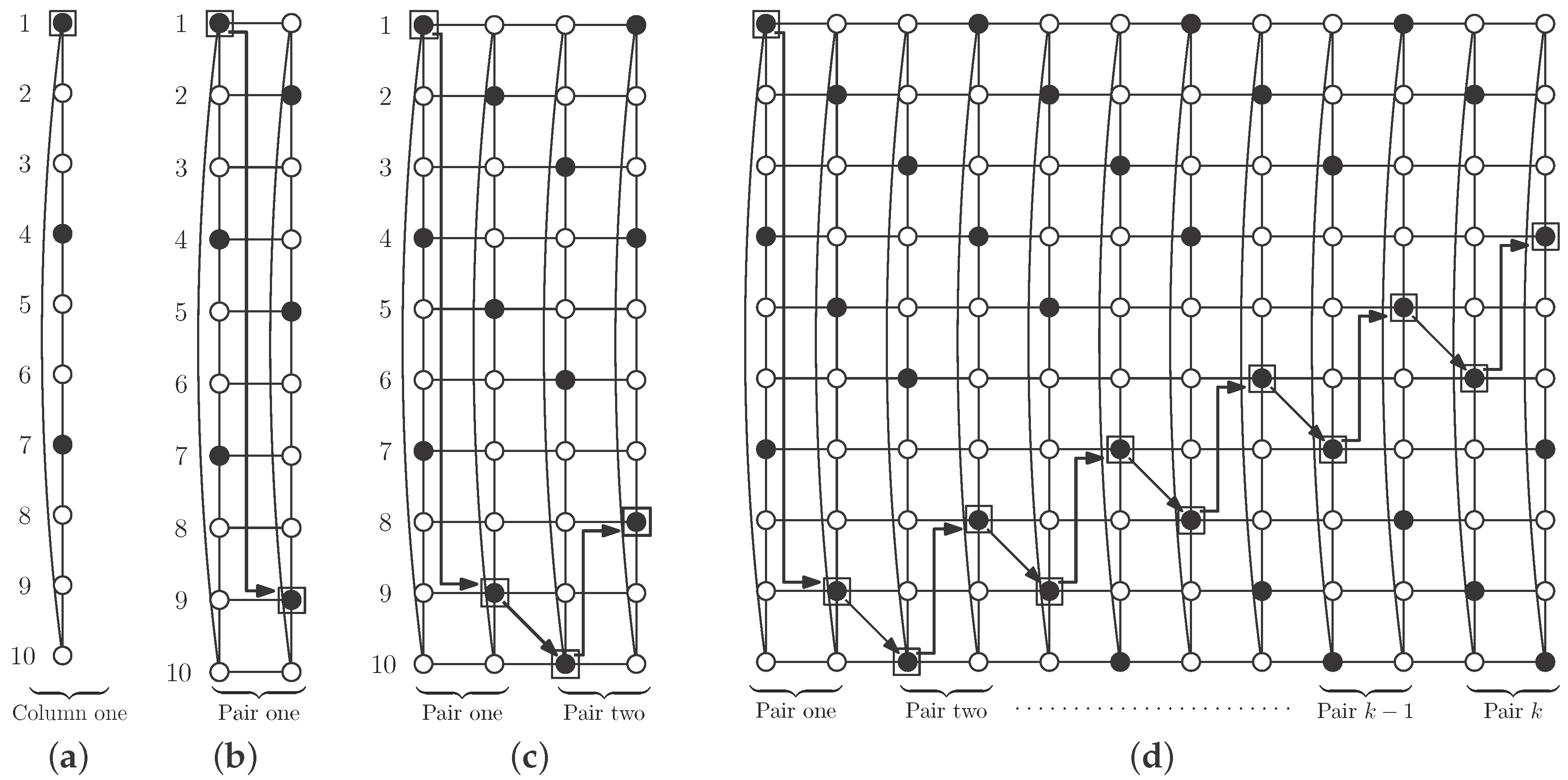
Case 2: .
To describe the pattern we use here, we begin with a single column. Vertices in
S in such a column are those in positions a multiple of three plus one, except the vertex in position
, so the column contains
r vertices in
S. We call the vertex in position one in the column the mark vertex, and, by construction, the mark vertex belongs to
S (see
Figure 9a, mark vertex with a square). We repeat this distribution of vertices in
S in the second column, but rotating the cycle in such a way that the mark vertex is in the position two units smaller (modulo
m) (see
Figure 9b, the arrow shows rotation). The set
S is an independent
-set in this pair of columns.
Consider now a new pair of columns with the distribution of vertices in
S described above. We join it to the preceding pair, and, in this case, we rotate the cycles so that the mark vertex is in position one unit larger (modulo
m) (see
Figure 9c, the arrows show rotations). Again, we obtain an independent
-set in the resulting cylinder. Repeating this operation as many times as necessary, we obtain an independent
-set
S in
(see
Figure 9d, the arrows show rotations).
We show in
Figure 9 an example with ten rows, but the construction also works for smaller cases (four and seven rows), and for bigger cases. Regarding the cardinality of
S, note that there are
r vertices of
S in each column, so
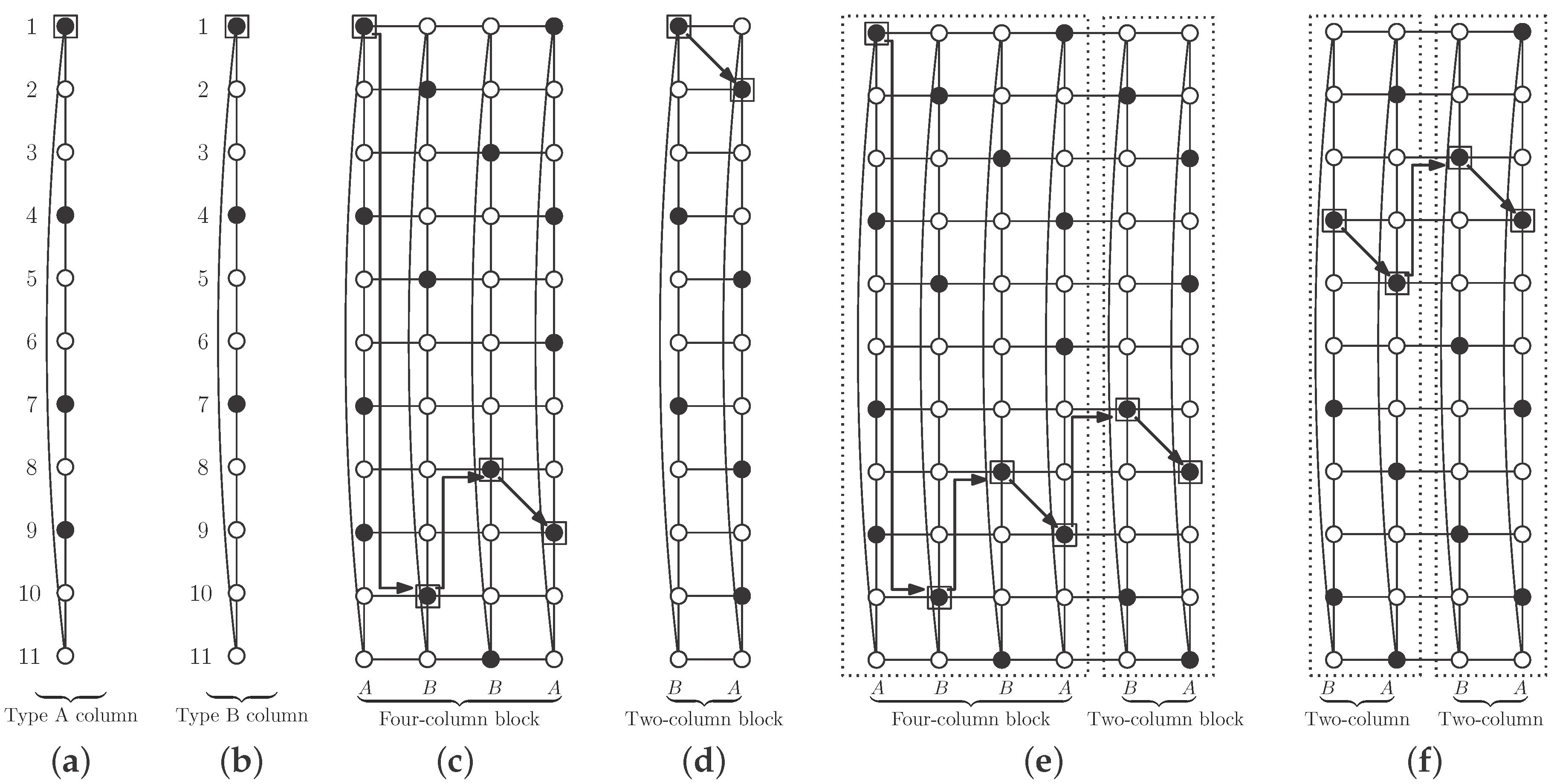
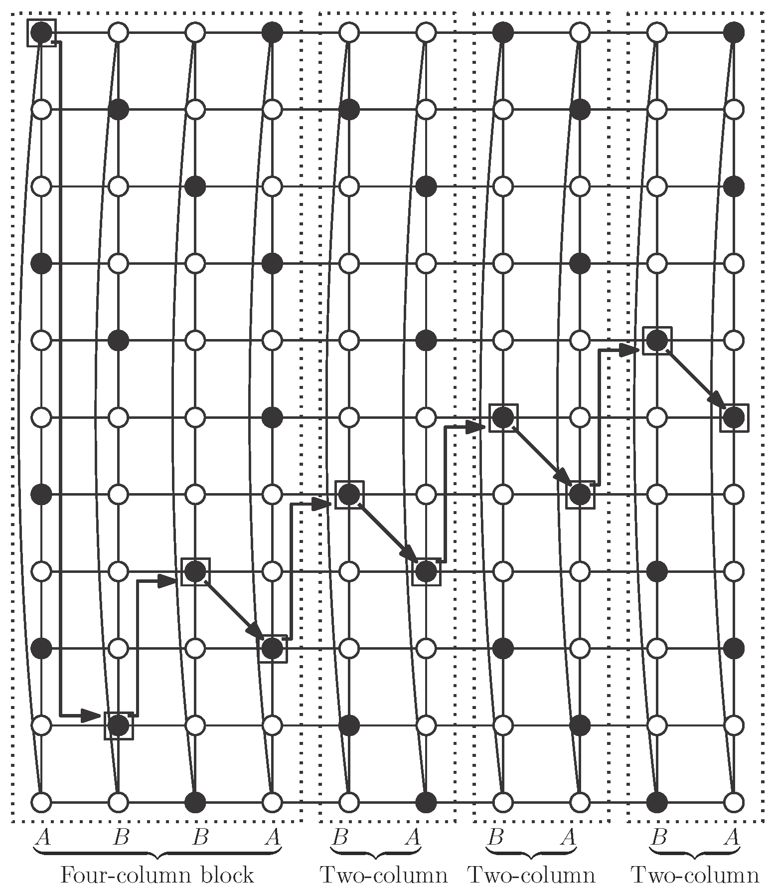
Case 3: .
We begin here with two types of columns. In Type A columns, vertices in
S are in positions multiple of three plus one, except in position
; in addition we include vertex in position
(see
Figure 10a). We call the vertex in position one in the column the Type A mark vertex, and, by construction, this vertex belongs to
S. Note that there are
vertices of
S in type A columns.
In Type B columns, vertices in
S are in positions multiple of three plus one, except in position
. We do not add any other vertex here (see
Figure 10b). We call the vertex in position one in the column the Type B mark vertex, which belongs to
S. In a Type B column there are
r vertices in
S.
Rules to join both types of columns, in order to obtain the desired independent
-set, are the following. We first need a four-column block, of types A, B, B and A (in this order), where each column is rotated, in reference to the previous one, until placing mark vertices as shown in
Figure 10c. Note that vertices in
S in this block are an independent
-set in the block.
We now make a two-column block by placing a Type B column and a Type A column (in this order), in such a way that mark vertices are in positions shown in
Figure 10d.
We place a two-column block after another block (with four or two columns), rotating the second block in such a way that its mark vertex is in positions shown in
Figure 10e,f.
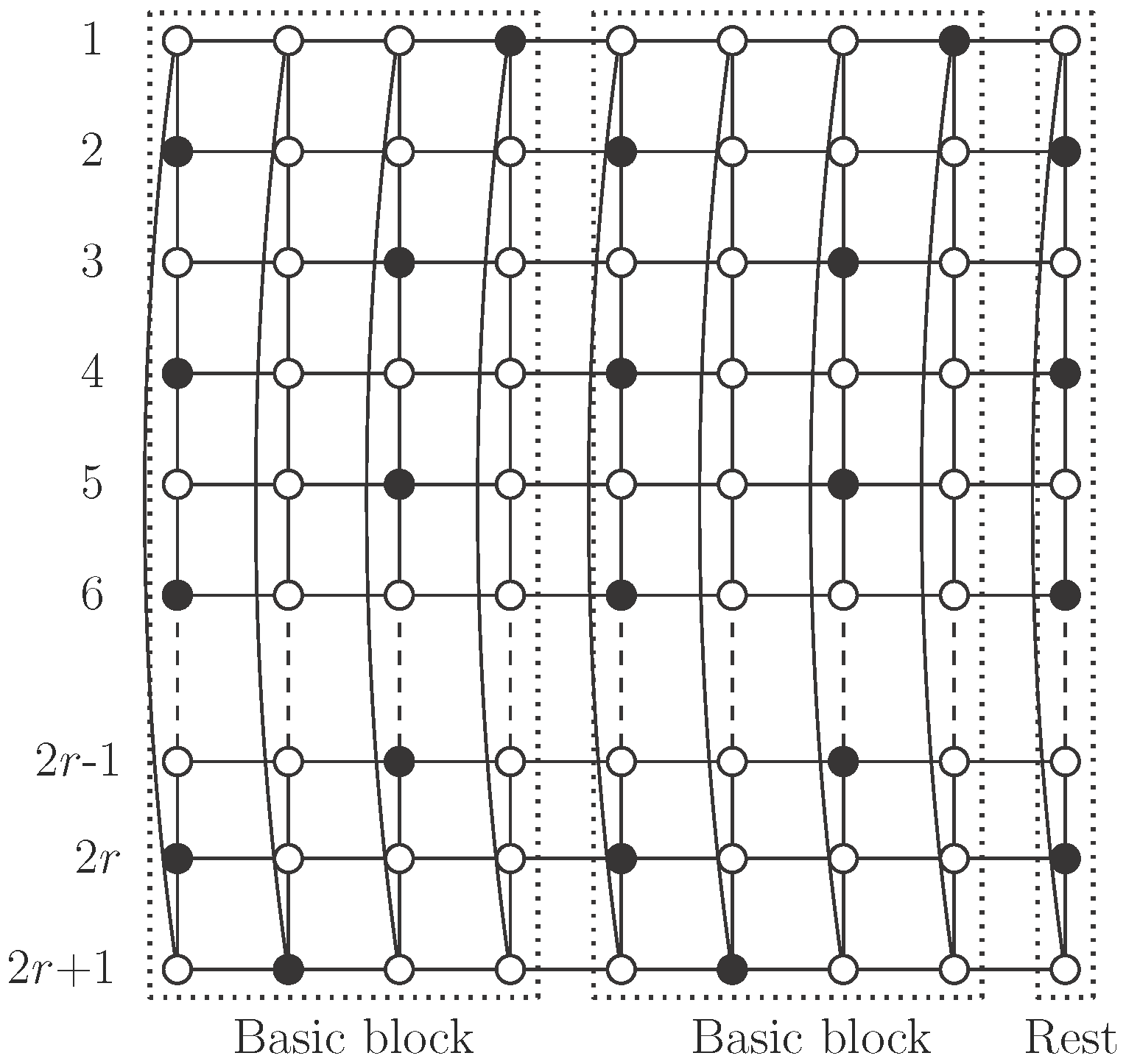
The desired independent
-set
S is obtained with one initial four-column block and attaching to it as many two-column blocks as necessary, to obtain the cylinder
(note that
) (see
Figure 11). Note that, although vertices in
S in a two-column block are not a dominating set by themselves, as can be seen in
Figure 10d, when we attach such a block to one four-column block following the rotation rules as described above, we obtain an independent
-set
S (see
Figure 10e). After this first operation, adding a new two-column block keeps independent
-domination (see
Figure 11). We show in this figure the case
, but the same pattern works with smaller cases
and
, and also with larger ones.
The four-column block contains two type A and two type B columns, so there are
vertices of
S in the block. On the other hand, two-column blocks consist of one type A and one type B column, so they have
vertices in
S. Finally,
S contains one four-column block and
two-column blocks, so:
3. Computing the Independent []-Number in Cylinders
Having proven that every cylinder, except
, has an independent
-set, in this section, we present an algorithm to compute the independent
-number in cylinders of small sizes. This is an adaptation of the algorithm presented in [
15], to compute the domination number of grids. A modified version of this algorithm also appears in [
16,
17]. Although the steps of the algorithm are quite similar to the original one, we prefer to completely described it, in order to fix notation and to point out the differences. We focus on cylinders
with
, because the case
was solved in Proposition 4.
The main tool of the algorithm is the
matrix multiplication. This is the standard matrix multiplication for the semi-ring of tropical numbers in the min convention (see [
18]), that is, the usual multiplication is replaced by sum, whereas the usual sum is replaced by minimization. Therefore, the
product of an
matrix
A and an
matrix
B is computed by the formula
. Moreover, the
product of a matrix
A and a scalar
c is computed by
.
The other key point of the algorithm is the identification of columns of the cylinder with words in the alphabet , in such a way that the number in each vertex describes its behaviour regarding independent -domination. We next describe how we will do this. Let be a cylinder and let be an independent -set. We identify each vertex u with an element of the set , following these rules:
if ;
if u has exactly one neighbor in S in its column or in the previous one;
if u has exactly two neighbors in S in its column or in the previous one;
if u has no neighbors in S in its column or in the previous one.
By definition, each vertex equal to 2 has at least one neighbor in S in its column and each vertex equal to 3 has a unique neighbor in S, which is in the following column. Every vertex in the cylinder is in exactly one of the preceding situations, so all of them can be identified with a unique number. Therefore each column can be seen as a word of length m in the alphabet , where the first and last letters are consecutive, because columns in the cylinder are cycles with m vertices. The property of set S being an independent -set provides a number of restrictions in words that can appear, which we list below. In all the restrictions, we consider that the first and last letters of the word P(≡ column) are consecutive, because each column is a cycle. If P is a word associated to an independent -set S, then P does not contain any of the following sequences:
- (a)
- (b)
- (c)
Note that any sequence of List (a) in a column implies that in the column, or in the previous one, or in the following one, there are two consecutive vertices of S, so it is not possible. Sequences in list (b) are not allowed because of the rules for associating each vertex with its number. Finally, sequences of list (c) do not appear in any column because each vertex has at most two neighbors in S and in all cases, such a sequence implies that in the previous column there is a vertex (next to the zero) with three neighbors in S. A word of length m in the alphabet not containing any of the sequences in Lists (a), (b) and (c) is called a correct word.
We also need to bear in mind that the first and last columns of the cylinder play a different role than interior ones, because they are placed next to a unique column, not between two columns. A word in the first column satisfies that every vertex equal to 1 has a neighbor in the column (just one) equal to 0, and every vertex equal to 2 has both neighbors in the column equal to 0. A correct word satisfying these conditions is called an initial word. On the other hand, the word in the last column does not contain any vertex equal to 3 and we call correct words satisfying this property final words.
Some restrictions regarding rows also arise. They can be described with rules that describe where a column P can be placed in the following position of column Q. In order to collect these restrictions, we denote letters in words P and Q as and and in the following cases, indices are taken modulo m,
- (i)
if , then either or ;
- (ii)
if , then either or or or ;
- (iii)
if , then either or ;
- (iv)
if , then .
If words P and Q satisfy Conditions (i) to (iv), we say that P can follow Q. Clearly, each independent -set in the cylinder can be identified with a unique ordered list , of n correct words of length m in the alphabet , such that
We denote such ordered lists as -lists. An ordered list satisfying properties 1 and 2 is called an -quasilist.
To compute the independent
-number of
, that is, the minimum number of zeros among all
-lists, we define the following vector. Denote by
the cardinality of the set
of correct words of length
m. The vector
, of length
, is defined as follows:
We also define the matrix
, a square matrix of size
such that
By multiplying vector
and matrix
A, with the
matrix multiplication, we obtain a new vector
, and, clearly, every finite entry
represents the minimum number of zeros among all
-quasilists having
as its second word. We can repeat this process as many times as we need, so if
, then every finite entry
, represents the minimum number of zeros among all
-quasilists having
as its last word. Having in mind that an
-quasilist whose last word is final is an
-list, we obtain
Moreover, algebraic properties of
matrix multiplication give the following result, which is similar to Theorem 2.2 of [
16].
Proposition 5. Let be an integer and suppose that there exist such that . Then for every , and moreover Proof. We prove by induction that
for every
. On the one hand,
by hypothesis. Assume now that
for
. Then, properties of the
matrix algebra and the inductive hypothesis give
Therefore, if
and
, then
for every index
i. In particular,
is finite if and only if
is finite. Finally this gives
Results presented in this section provide the following algorithm to compute the independent
-number of
. It is an adaptation of the algorithm presented in [
15], to compute the domination number of grids. A modified version of this algorithm also appears in [
16,
17]. On the one hand, the algorithm computes the value of
for fixed and small enough
. On the other hand, given a fixed
m, it computes a list of vectors
and it tries to find the recurrence relationship on the hypothesis of Proposition 5.
If a recurrence is found by Algorithm 1, Proposition 5 provides a finite difference equation
with
d boundary values
. The solution of this equation is
where the value of
depends on the boundary values. Remaining values of
, that is for
, have also been computed by the algorithm, so finding the recurrence means that the independent
-number of
is completely computed.
| Algorithm 1: Recurrence for the Independent -number in Cylinders |
![Symmetry 10 00024 i001]() |
However, the existence of such a recurrence relationship is not guaranteed, as was mentioned in Section 6 of [
15]. Some sufficient conditions on an arbitrary matrix
A, in the
matrix algebra, are known that ensure such a recurrence exists. We recall the following definition from [
15]. A matrix
A is
irreducible if there exists an integer
K such that for every
, matrix
has no infinite entries, and this is analogous to the definition of irreducible matrix in regular matrix algebra. Theorem 6.3 of [
15] states that, if
A is an irreducible matrix, then the recurrence needed to apply Proposition 5 occurs.
The following characterization is well known; see, for instance, [
19]. Considering matrix
A as the adjacency matrix of a directed graph (there is an arc from
j to
i if and only if
),
A is irreducible if and only if such a directed graph is strongly connected. In particular, a matrix such that every entry in the
row is equal to
is not irreducible, because no arc arrives to
i. When this situation happens, the recurrence needed in Proposition 5 could not occur.
This is the main difference between the computation of the independent
-number in cylinders and the previous cases where this algorithm has been used (see [
15,
16,
17]). In our case, matrices defined using the properties of independent
-sets have an increasing number of rows with no finite entry, when
m gets larger. In fact, we just found the desired recurrence in cases
and
. If
our strategy consists of modifying the first step of the algorithm. We consider a reduced collection
of correct words instead of having all of them, so we obtain an auxiliary parameter
that represents the minimum number of zeros among all
-lists with words in
, if there exists at least one of such
-list. Then, we use the algorithm to look for the recurrence relationship, but using just correct words in subset
and, in the case it is found, the auxiliary function obtained satisfies
. The final step consists of combining this upper bound with an appropriate lower bound, in order to localize the independent
-number in an interval as small as possible.
4. Experimental Results
In this section, we present the results obtained with Algorithm 1, for values of
m between 4 and 15. The link to the source code, in programming language C, to perform all the operations described in the algorithm can be found in the
Supplementary Materials. Notice that vector
is computed using its definition, but vectors
are obtained by successively multiplying matrix
A and vector
, with the
matrix multiplication. We do this operation by means of an adaptation of the CSPARSE library [
20]. This library provides a fast method for multiplying sparse matrices with the usual product, and we have adapted it for the
matrix product. Therefore, we have obtained a library that efficiently multiplies sparse matrices, also with this product, as can be seen in
Table 1, where we show that execution times for computing the first 100 vectors are shorter than times for the computation of the matrix. We have also included computation times for the set of correct words, but not for vector
, because it is less that one second in all cases.
4.1. Cases 4 and 5
In both cases, we have found the recurrence needed to apply Proposition 5, and we have completely computed the independent
-number of cylinders
, for
. Data obtained with Algorithm 1 and finite difference equations appear in
Table 2.
The solution of the finite difference equation gives the formula of the independent
-number. In both cases, the independent
-number agrees with the domination number (see [
12]); therefore, independent
-sets provide the most efficient way to dominate these cylinders.
4.2. Cases 6 10
In these cases, matrices obtained with the algorithm have a large number of rows with all entries equal to , so they are not irreducible. This means the recurrence is not guaranteed and, in fact, we have not found it in the first 100 vectors. Clearly, it could happen that the recurrence relationship exists for some , but instead of keeping on looking for a recurrence in larger values, we prefer a different approach.
We remove a group of correct words and we use Algorithm 1 again, but considering the remaining word subset instead of the complete list of correct words computed in step 1. The criterion for removing words takes into account formulas for the independent domination number
obtained in [
14], and we look for similar formulas for the independent
-number. We fixed vector
because it is small enough to quickly use the algorithm and it gives positive results in cases we are considering. For each
m, we take the integer
d in formula
and we study the pair of vectors
. Their entries in the
position,
, are in one of the following situations:
both are infinite;
both are finite, then we compute the difference ;
one of them is finite and the other one is infinite, then we say that they are non-comparable.
If a recurrence is not found, then either there are non-comparable pairs or differences of finite entries are not equal, or both. In
Table 3, we show values of differences found and if there are non-comparable words. Recall that, for each
m, the set of correct words
is ordered and it has
elements, and the size of vector
is
. We now take the integer
c in
and we keep the word in position
i if both
entries are finite with
and also in case
. However, we remove the word in position
i if entries are finite with
or
are non-comparable. This strategy provides a subset
of correct words that we use in the algorithm, instead of the complete list originally computed in the first step. In cases
, we found the recurrence, as we expected. However, in case
, after a first selection of words, recurrence does not appear and we remove a second group of words, with the same criterion. It is shown in
Table 3, in rows 10-I and 10-II. After removing the second word group, a recurrence also appears for
.
We now apply Algorithm 1, but using the subset of remaining words instead of the complete list. We would like to point out that there exists an -list with words in if and only if the value of is finite, where , is the initial vector, A is the matrix, both associated to subset of correct words of length m, and . Clearly, if this auxiliary function is finite, then it provides the minimum number of zeros among all -lists with words in , so it is trivially true that . Moreover, if we just consider words in and the recurrence relationships described in Proposition 5 occurs, then the finitude of boundary values ensures that is finite, for every .
Recurrences and boundary values found by Algorithm 1, when we just use the subset
of correct words described in
Table 3, are shown in
Table 4.
The solutions of auxiliary equations are the following:
As we mentioned before,
is an upper bound of the independent
-number of
, and we now combine these results with the values of
[
14], which is a natural lower bound, that is
In cases and also in case , we obtained , so the independent -number agrees with the independent domination number. In case and , we obtained ; the bounds do not agree and we can just conclude that . We computed the independent -number for and it agrees with the upper bound in all cases.
We also computed the independent
-number of small cylinders (
) with the algorithm, by using Equation (
2) with the complete list of correct words. We include these values in the final formulas.
, if and
, if .
4.3. Cases 11 15
In these cases, the independent domination number is not known, so our first task is to compute it. We will use these values as a lower bound of the independent
-number. To this end we have implemented the algorithm described in [
16], to compute the independent domination number of the grid
, making the necessary changes to adapt it to the cylinder
. These changes just consist of considering that the first and the last letters in each word are neighbors. Computations can be done following the same steps as in Algorithm 1, but taking into account the rules to define correct words and to compute vector
and matrix
A that correspond with the definition of independent domination. For the sake of completeness, we recall these rules from [
16]. For an independent dominating set
S of
, each vertex
is identified with an element of the set
, following these rules:
if ;
if u has at least one neighbor in S, in its column or in the previous one;
if u has no neighbors in S, in its column or in the previous one.
Each column in can be seen as a word of length m in the alphabet , where the first and last letters are consecutive. Correct words are those words not containing the sequences . For a pair of correct words , we say that can follow if they satisfy the following conditions
- (i)
if , then ,
- (ii)
if , then either or or ,
- (iii)
if , then .
Following the same steps as in Algorithm 1 with the rules described above, recurrence is found for and we present the final formulas obtained (we have not included small cases not following the general formula).
We now follow the same strategy as in the preceding cases and we use vectors
because they provide positive results in all cases. For
, the first reduction of the correct words gives positive results and we found the recurrence. However, in case
, after a first selection of words, a recurrence does not appear and we remove a second group of words, with the same criterion. After removing the second word group, a recurrence also appears in this case. We show the rules for reducing the correct word set in
Table 5. In
Table 6, we show recurrences and finite difference equations in each case.
Solutions of auxiliary equations are the following
Final formulas have been obtained by comparing auxiliary equations with the above computed independent domination number and by using inequalities . We also include values for small cylinders, with . In the case , we also include values of for .
, if and
5. Conclusions
In this paper, we have deeply studied independent -sets and their associated parameter, the independent -number, in cylindrical networks. The main interest of this study lies in the known fact that the cylinder has an efficient dominating set if and only if and , so in other cylinders different domination-like sets are needed to dominate them as efficiently as possible. On the other hand, the symmetry of these graphs allows us to focus their study from different points of view.
In
Section 2, we have proven that every cylinder
with
has an independent
-set. We also provided exact values of
and
and upper bounds for the independent
-number in the rest of the cases.
In
Section 3, we presented an adaptation of a known algorithm to compute exact values of
; and we presented the experimental results obtained with the algorithm in
Section 4, for
. To this end, we have adapted the CSPARSE library, a fast method for multiplying sparse matrices, to the case of
multiplication and we have introduced the technique of selecting some correct words when using the algorithm, providing new possibilities of applying this type of recursive computing in cases where the matrix is not irreducible and a recurrence is not found.
Regarding the cases in which we have exactly computed the independent
-number, comparing our results with the values of the domination number [
11,
12] and leaving aside the small values of
n not following the general formula, we may conclude that:
if , then ;
if , then ;
if , then ,
;
.
Summing up, it is known that, in general, the independent -number does not equal the domination number; however, we have seen that there are some cylinders having this property and some others where both parameters differ by 1. In view of these results, we may conclude that independent -sets provide an interesting alternative to efficient dominating sets in cylindrical networks.


