Mapping Flood-Based Farming Systems with Bayesian Networks


1
World Agroforestry Centre (ICRAF), United Nations Avenue, Gigiri, Nairobi 30677, Kenya
2
Department of Environmental Sciences, Kenyatta University, Kenya Drive, Nairobi City 43844, Kenya
3
University of Bonn, Department of Horticultural Sciences, Auf dem Hügel 6, 53121 Bonn, Germany
4
Center for Development Research (ZEF), University of Bonn, Genscherallee 3, 53113 Bonn, Germany
*
Author to whom correspondence should be addressed.
Land 2020, 9(10), 369; https://doi.org/10.3390/land9100369
Submission received: 23 August 2020
/
Revised: 25 September 2020
/
Accepted: 29 September 2020
/
Published: 2 October 2020
Abstract
:Many actors in agricultural research, development, and policy arenas require accurate information on the spatial extents of cropping and farming practices. While remote sensing provides ways for obtaining such information, it is often difficult to distinguish between different types of agricultural practices or identify particular farming systems. Stochastic system behavior or similarity in the spectral signatures of different system components can lead to misclassification. We addressed this challenge by using a probabilistic reasoning engine informed by expert knowledge and remote sensing data to map flood-based farming systems (FBFS) across Kisumu County in Kenya and the Tigray region in Ethiopia. Flood-based farming is an important form of agricultural production employed in regions with seasonal water surplus, which can be harvested and used to irrigate crops. Geographic settings for FBFS vary widely in terms of hydrology, vegetation, and local practices of agronomic flooding. Agronomic success is often difficult to anticipate, because the timing and amount of flooding usually cannot be precisely predicted. We generated a Bayesian network model to describe the FBFS settings of the study regions. We acquired three years (2014–2016) of Moderate Resolution Imaging Spectroradiometer (MODIS) Terra spectral data as eight-day composite time series and elevation data from the Shuttle Radar Topography Mission (SRTM) to compute 10 spatial data metrics corresponding to 10 of the 17 Bayesian network nodes. We used the spatial data metrics in a fully probabilistic framework to generate the 10 spatial data nodes. We then used these as inputs for the probabilistic model to generate prior and posterior spatial estimates for specific metrics along with their spatially explicit uncertainties. We show how such an approach can be used to predict plausible areas for FBFS based on several scenarios. We demonstrate how spatially explicit information can be derived from remote sensing data as fuzzy quantifiers for incorporating uncertainties when mapping complex systems. The approach achieved a remarkably accurate result in both study areas, where 84–90% of various FBFS fields sampled were correctly mapped as having a high chance of being suitable for the practice.
1. Introduction
Flood-based farming systems (FBFS) are rainfed farming systems that occur in dryland areas and rely on supplementary water derived from various types of floods. Herein, floods are understood in terms of natural variability such as the rise of water in reservoirs (e.g., rivers, lakes, or dry wadis) during the periods of high water [1,2]. They should not be confused with flood disasters, but seen as a source of water farmers use to irrigate crops by virtue of agronomic flooding [3]. In some areas, farmers invest substantial effort to build and maintain complex physical infrastructures for water acquisition and sharing [4]. In other areas, farmers invest relatively little effort, since they deliberately plant crops on flood-prone lands to be naturally irrigated by the coming floods, or on residual moisture from previous flooding [2]. FBFS usually occur in relatively low-lying areas with gentle topography. Various forms of FBFS are found across the world’s drylands, including many locations where farmers have been relying on these systems for centuries [2,4,5,6]. Water supply in FBFS is often difficult to predict due to uncertainties in the timing, duration, size, and frequency of floods [3,4]. Depending on the type of biophysical environment, FBFS are characterized by specific social and institutional arrangements that govern water allocation [4,5,7,8]. By making flood water available for use in agriculture, these farming systems contribute to food security and deliver many other benefits [4] for millions of people in a wide range of geographies [7,9].
Many countries across Africa and Asia support the development of FBFS through the Flood-Based Livelihood Network (FBLN), which represents a common framework for research, policy, and action [9]. The FBLN initiative aims to share knowledge and improve the productivity of FBFS. To achieve its objectives, the FBLN, as well as decision-makers at local to national levels, require accurate information on FBFS to map their extent, monitor their development over time, and assess their benefits to societies at various scales, highlighting the need for adequate methodologies to map them.
Despite their importance, FBFS have been the topic of surprisingly few studies [4,6]. While these studies have made substantial contributions towards the understanding of important aspects of FBFS (e.g., hydrology and sedimentation, design and maintenance, social and institutional arrangements), little effort has been made to provide reliable estimates of the spatial extent of FBFS. The large uncertainties in the estimates of the spatial coverage of FBFS [3,4] indicate that reliable mapping approaches specific to FBFS settings are still needed. Mapping approaches tailored to FBFS can benefit from considering the three important aspects known to characterize most FBFS settings [3,4,7]:
- The diversity of FBFS settings: the diversity of FBFS settings in terms of floodwater availability, crop types, or social organization (e.g., spate irrigation in Tigray versus inundation canals in Kisumu) suggests that diagnostic elements aiming to operate at large scale should be framed into a conceptual model that can be applied in a wide range of contexts.
- The similarity of FBFS with other ecological systems: FBFS systems share characteristics with other ecological systems. They are similar to conventional irrigation in terms of supplementary irrigation, they resemble rainfed agriculture in terms of rainwater and growing period, and they share features with riparian vegetation in terms of extended growing period. These similarities indicate that valid concepts should be translated into flexible classification rules that can be used to highlight the most outstanding features of FBFS and discriminate them from the other ecological systems.
- The unpredictable nature of floods in FBFS: the large uncertainty in FBFS estimates, particularly in the areas these farming systems cover, implies the need for an approach that can detect agronomic flooding even in situations where flood events are not physically observable on satellite images. This is important because flood events may not leave a detectable trace of inundation, not only because the sensor can miss the flood event, but also because many FBFS have deep soils capable of storing large volumes of water. Agronomic flooding may also occur after the planting date, in which case it can be confused with other types of flood events because flood occurrence is largely unpredictable, and it is difficult to determine whether and how floods are used for FBFS purposes [3,4].
The wealth of satellite remote sensing data and the advances in algorithms for processing these data [10,11,12,13,14,15,16,17] provide an opportunity for describing important FBFS characteristics in a spatially explicit manner. Diagnostic elements such as typical FBFS vegetation, hydrology, and topography can be derived from available satellite images as spectral indices and topographic structures. These can be used to feed geospatial models and estimate the spatial coverage of FBFS in a wide range of settings.
The objective of this paper is to provide a mapping routine to comprehensively estimate the coverage of FBFS. We propose a methodology to identify relevant spatial and nonspatial information for characterizing FBFS without omitting sources of uncertainty. We use a multivariate model of causality to leverage both available data and expertise [18,19,20,21]. We use expert elicitation techniques to identify variables that are relevant for characterizing FBFS, and a wide range of spectral metrics to relate these variables to remotely sensed data. We apply probabilistic models that consider uncertainties and causal relationships [22,23]. We describe how this can be achieved and how to derive the required inputs for Bayesian networks from raw spatial data. We successfully applied the proposed approach in two areas with distinct geographic settings, Kisumu County in Kenya and the Tigray region in Ethiopia.
2. Materials and Methods
2.1. Study Area
FBFS are being incorporated into national plans for agricultural development in both Kenya and Ethiopia [9]. A generic mapping approach suitable to FBFS settings could inform policy and help to assess and monitor the spatial coverage of the practice. We demonstrate this potential based on Kisumu County in Kenya and the Tigray region of Ethiopia where the practice of FBFS has strong economic and cultural importance. Both regions have long histories of flood-based agriculture but differ in the way floods are managed for agricultural purposes (Figure 1).
Kisumu County extends between 33°20’ E and 35°20’ E and 0°20’ S and 0°50’ S, covering an area of 2009.5 km2, of which 567 km2 (28.2%) is covered by water [24]. The central part of the county is relatively flat, surrounded by ridges reaching up to 1835 m above sea level. The relief of the county can be classified into three main topographic regions: the Kano lowland plains, the Maseno midlands, and the highlands of the Nyabondo Plateau. The Nyabondo Plateau constitutes the bulk of the area that is prone to flooding, particularly during periods of heavy rains. The floodplains are well suited for agriculture due to their relatively rich soils that have been formed by recurrent alluvial deposits.
Tigray is a region in northern Ethiopia between 36°27’ E and 39°59’ E and 12°15’ N and 14°51’ N. The region shares the north-western highlands of the main Ethiopian rift valley with the Amhara region. The altitude increases from north-east (500 m) to south-west (nearly 4000 m) along an escarpment that marks the edge of an extensive highland plateau.
Flood-based agriculture in Tigray differs from that in Kisumu in several ways (Figure 1). While most of the water sources for FBFS in Kisumu are permanent water bodies, those in Tigray are mainly dry wadis. Floods are of relatively short duration and less frequent in Tigray than in Kisumu. This makes Tigray more suitable for spate irrigation (i.e., irrigation systems that rely on runoff) compared to Kisumu, where most FBFS rely on inundation canals (i.e., irrigation systems that rely on floods in water bodies and floodplains). Spate irrigation soils in Tigray are predominantly loamy, and the vegetation is relatively sparse compared to Kisumu, where most FBFS soils have relatively high clay contents.
2.2. Conceptual Framework
We used a conceptual approach that considers important assumptions in relation to major characteristics of FBFS [4,7]. We built a probabilistic framework to differentiate FBFS from other ecological systems using satellite remote sensing. While FBFS present many similarities with other ecological systems, FBFS settings are highly variable. Therefore, we used imprecise quantifiers in a multicriteria framework, using imperfect knowledge to describe important FBFS features. We used a Bayesian network to automate these concepts and characterize the settings of FBFS using partially informative variables, which we described using discrete states quantifying relative proportions in common language (e.g., low, medium, high).
Bayesian networks are reasoning engines that can be used to model partially understood processes using probability, hence allowing for the incorporation of uncertainties in the analysis [25]. They are causal probabilistic models that can be used to decompose large joint probability distributions [25,26,27]. In the context of ecological remote sensing, the ability to incorporate new information into Bayesian networks [26] makes them useful for monitoring system pathways.
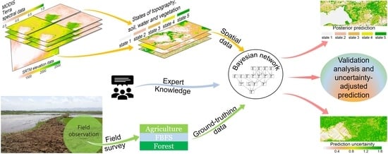
Assuming that some FBFS features may not be available as satellite images, we programmed the Bayesian network to accept both spatial (discrete raster) and nonspatial (multinomial probability distributions) data and used the model to predict FBFS potential based on the states of soil, water, vegetation, and topography (Figure 2). To automate the process, we first identified the study area in a geographic information system to acquire the spatial data. We then processed the MODIS and the SRTM data to compute several spatial data metrics based on the specifications of the Bayesian network and the type of data (e.g., single or multilayer raster). To account for the states of the different variables in the Bayesian network, we adopted a procedure that uses spatial (for both single and multilayer raster) and temporal variability (for multilayer raster only) to discretize the data. While the Bayesian network accepts both spatial and nonspatial data inputs, it always produces thematic predictions along with their uncertainties in a spatially explicit manner. The main idea consisted of reducing uncertainty along the Bayesian network topology such that the lowest possible uncertainty is achieved towards the node ‘FBFS potential’, which expresses the suitability of a given pixel for FBFS. For example, while wet soils are more likely to characterize FBFS settings compared to dry ones, the confidence in making this call would be higher if we also knew that the area had a gentle slope and high flow accumulation. Despite these water and topographic indicators, the area would not be identified as suitable for FBFS without evidence of vegetation.
Based on the available literature, field work, and expert and farmer consultations, we used a set of 17 variables (see Figure 3) to describe the states of each pixel. Based on the specifications of the Bayesian network, we acquired satellite images to compute 10 spatial data metrics based on which we generated 10 spatial data nodes. These nodes were used to feed the Bayesian network. We conducted the data analysis using the R programming language [28]. To explicitly describe the methodology, we developed computer programs described in the R packages growingSeason and spatialProbs along with a reproducible workflow of the analysis (see Supplementary Materials).
2.3. Acquisition of Nonspatial Data and Bayesian Network Specifications
We reviewed the essential literature related to the topic of FBFS and conducted high-level discussions with 11 experts to draft the Bayesian network, which we then cross-checked based on farmer consultations and field observations. While the Bayesian network is essentially based on the expert-elicited data, we integrated the information acquired from the literature review and the discussions with the farmers to formalize the Bayesian network into a computer-readable model [29]. The literature review mostly focused on the FBLN database [9] and contributed to resolving conflicting points of view among experts. The field work and the discussions with the farmers mainly aimed at checking the validity of the probability distributions and the graphical structure of the model. To feed the Bayesian network, we generated 10 nodes as spatial data (i.e., Slope, Flow accumulation, Vegetation sensitivity to water variation, Surface sensitivity to flooding, Soil water content, Surface exposure to wetness, Temporal variation in vegetation, Water presence, Flood at the beginning of the rainy season, and Power of tools). We then used the Bayesian network to predict the likelihood of a pixel’s potential for FBFS (Figure 3, FBFS potential) based on the topographic suitability of the pixel for FBFS (Figure 3, Suitable topography), the presence of vegetation within the pixel (Figure 3, Vegetation presence), the potential of the pixel for floodwater (Figure 3, Flooded at some point), the variation of vegetation due to flood at the pixel (Figure 3, Vegetation variation due to flood), and the quality of the data (e.g., cloud cover and pixel quality assessment) used to feed the Bayesian network (Figure 3, Power of tools).
To define the topographic suitability of a given pixel to FBFS, we assume that the flow accumulation determines the amount of floodwater reaching the pixel and the slope determines whether the water will be retained or pass through the pixel. We assessed the presence of vegetation within the pixel through the pixel potential for typical FBFS vegetation (Figure 3, Characteristic vegetation), which results from vegetation sensitivity to water variation (Figure 3, Vegetation sensitivity to water variation) and surface sensitivity to flooding (Figure 3, Surface sensitivity to flooding). Considering that vegetation variation can occur even in areas where flooding is uncommon, we attributed vegetation variation to floodwater at a pixel (Figure 3, Vegetation variation due to flood) based on the presence of water on the ground (Figure 3, Water presence), vegetation seasonality (Figure 3, Temporal variation in vegetation), and the likelihood of flood events around the beginning of the growing season (Figure 3, Flood at the start of the rainy season). We assumed that the pixel’s moisture content (Figure 3, Soil water content), its exposure (Figure 3, Surface exposure to wetness), and sensitivity to flooding (Figure 3, Surface sensitivity to flooding) jointly affect water presence and vegetation seasonality. We estimated the pixel potential for floodwater based on characteristic vegetation, water presence, and soil suitability for FBFS (Figure 3, Suitable soil) considering that water presence can be common in areas where soils are not suitable for agriculture (e.g., water bodies, encrusted soils). We assumed that soil suitability depends on soil water content and surface exposure to wetness.
2.4. Acquisition and Preprocessing of Spatial Data
To derive the spatial data metrics corresponding to the spatial data nodes in the Bayesian network, we acquired void-filled digital elevation data from the Shuttle Radar Topography Mission (SRTM) sensor [30,31], and time series (2014–2016) of version VI data from the Moderate Resolution Imaging Spectroradiometer (MODIS) sensor [32]. We also acquired several polygon shapefiles which we used for both exploratory and validation analyses.
We acquired the administrative boundaries of the study regions as shapefiles from the Global Administrative Areas database [33,34], the SRTM version 4 data from the CGIAR Consortium for Spatial Information database [35], and the MODIS product MOD09A1 [36] from the NASA LP DAAC (Land Processes Distributed Active Archive Center). The SRTM version 4 provides elevation data at 90 m spatial resolution, and the MOD09A1 provides spectral bands of MODIS Terra as 8-day composites at 500-m spatial resolution [36]. While transient events (e.g., flash floods) can be overlooked considering the 8-days composites, MOD09A1 is the best publicly available MODIS product that provides a reasonable compromise between spatial and temporal resolution for our specific application [37]. We used the MODIS H/V tiles h21v09 and h21v08 for Kisumu County and h21v07 for the Tigray region to acquire the atmospherically corrected bands, based on which we [38] computed a total of six normalized difference spectral indices (Table 1) to evaluate moisture and vegetation [37,38]. We discarded all pixel values beyond the valid range ([−1, 1] for normalized difference spectral indices) and interpolated them over time [39].
While this collection of indices may seem redundant, it allowed us to exploit information from different parts of the electromagnetic spectrum, to compensate for imprecision and to reduce uncertainties in data estimates. We used the NDVI as a proxy for assessing vegetation cover and the NDFI for estimating flood depth. We used the NDII6 and the NDII7 to evaluate the water content in leaves, soil, and open water from different perspectives. We considered the Gao NDWI to be more inclined towards vegetation water, as opposed to the McFeeters NDWI, which we considered more suitable for assessing soil and surface water. High values of these spectral indices indicate high likelihood of the respective surface features being present (e.g., high NDVI values indicate active vegetation) [33,34].
2.5. Exploratory Analysis of the Normalized Difference Spectral Indices
To understand the temporal variability in flooding and vegetation, we examined the temporal profiles of the NDVI, the Gao NDWI, and the NDFI. We extracted data from 10,000 pixels, based on random sampling [34] to produce boxplots showing the temporal distribution of floods and vegetation in the study regions. We also conducted principal component analyses [40] to examine the spatiotemporal patterns of major floods and vegetation in the study regions. Based on the analysis of the scree plot of eigenvalues [41], we considered two principal components for Kisumu and seven for Tigray. We used the ground-truthing data to screen for potential thresholds for discriminating FBFS using a comparative analysis of the normalized difference spectral indices across different land use types. We also examined the temporal profiles of these major landscape features. These exploratory analyses suggested the use of imprecise quantifiers, owing to the similarity in the spectral response of FBFS and the other land cover classes considered.
2.6. Computation of Spatial Data Metrics
We used the elevation and spectral index dataset to compute several intermediary spatial data metrics, based on which we computed the 10 spatial data nodes describing topography, soil, water, and vegetation of the study regions. We computed the metrics corresponding to the nodes related to topography (i.e., slope and flow accumulation) using TauDEM software version 5.3 [42,43,44] from R [28]. We systematically computed the spatial data metrics corresponding to the spatial data nodes related to soil, water, and vegetation using one or several of the normalized difference spectral indices. We describe the spatial data metrics in more detail in the following sections. Note that we performed the computations of the spatial data metrics involving the normalized difference spectral indices throughout the time series.
2.6.1. Slope and Flow Accumulation
We computed the spatial data metrics related to the nodes ‘Slope’ and ‘Flow accumulation’ (Figure 3) following a three-step conditioning procedure. This included filling of the depressions in the original digital elevation model such that pixels formed a monotonically decreasing path that allowed adequate flow routing. We then derived slope and flow directions from this depression-less digital elevation model, and computed flow accumulation [14,15]. In filling the depressions, we fully accommodated for simple and looping depressions [14,42]. We computed the slope as the drop distance (tangent of the slope angle), from which we derived the D-infinity flow direction as the direction water exits a given pixel based on the ‘single flow direction’ concept [15,43]. This concept assumes that water exits a given cell in a single direction as opposed to the concept of multiple flow directions, which assumes that water can exit a given cell in more than one direction. Based on the derived flow directions, we computed the flow accumulation at each pixel as the number of pixels draining into it.
2.6.2. Vegetation Sensitivity to Water Variation
We estimated the metric related to the node ‘Vegetation sensitivity to water variation’ (Figure 3) using the NDII6, NDII7, and the NDVI, as the ratio between the potential moisture and the amount of vegetation (Equation (1)), based on the assumption that flooding followed by a rapid increase in vegetation [17] characterizes most FBFS settings. Therefore, vegetation in FBFS-like areas is likely to exhibit high absolute standard deviation due to the high variability in vegetation caused by seasonal flooding. In addition, the quasi absence of perennial vegetation in most FBFS settings stipulates that vegetation can be very low during the dry season. We used this metric to describe the temporal relationship between water and vegetation based on the proportion of vegetation relative to the amount of floodwater received at each pixel. This implicitly provides an estimate of the soil conditions, because the combination of low vegetation and high water presence may imply the presence of bare or swampy soils where vegetation may be sensitive to water variation.
where VegSensWateri is the vegetation sensitivity to water variation at pixel i, and n is the total number of images in the time series, sd is the standard deviation. NDII6i, NDII7i, and NDVIi, respectively, are the NDII6, NDII7, and the NDVI time series at pixel i.
2.6.3. Surface Sensitivity to Flooding
We estimated the ‘Surface sensitivity to flooding’ metric (Figure 3), based on the assumption that surface states (e.g., vegetation cover, soil surface roughness, soil crusting) influence the amount of locally generated runoff leading to flooding at larger scales. We computed the metric as the coefficient of variation of the NDFI (over time) to estimate how much variation in floods can be expected at each pixel (Equation (2)). Implicitly, this metric describes the relationship between water and soil. For example, areas permanently covered by water would have high NDFI values, with little temporal variation in these NDFI values, hence little sensitivity to flooding. In contrast, dry but flood-prone soils would have high sensitivity to flooding due to their potentially high temporal variation in flood index.
where SurfSensFloodi is the surface sensitivity to flood at pixel i, NDFIi is the NDFI time series at pixel i.
2.6.4. Soil Water Content
We computed the spatial data measuring ‘Soil water content’ (Figure 3) by aggregating the NDII6, the NDII7, the NDVI, and the NDFI (Equation (3)) based on the assumption that the overall water for crops is composed of water in leaves (NDVI, NDII6, and NDII7), water on the ground (NDFI) and water in soil (SWC). We used the NDII6, the NDII7, and the NDFI to take the greatest possible advantage of the NIR and SWIR spectral domains.
where SWCi is the soil water content at pixel i, and n is the total number of images in the time series. NDII6i, NDII7i, NDFIi, and NDVIi, respectively, are the NDII6, NDII7, NDFI, and the NDVI time series at pixel i.
2.6.5. Surface Exposure to Wetness
We estimated the spatial data metric related to the ‘Surface exposure to wetness’ node (Figure 3) as the sum of the NDFI over the time series, based on the assumption that FBFS experience more flooding compared to other land use types. Therefore, we used this metric to estimate the expected total water at a pixel and express the degree to which that pixel is exposed to flooding. This differs from the soil water content metric in that it estimates the surface soil water availability, regardless of whether this water is used by vegetation. We postulated that a certain amount of water may be detected at a given pixel at some point in time without necessarily being sustained, since water can quickly infiltrate through porous soils or stagnate on saturated or impermeable soils. On soils with high water holding capacity, a relatively small amount of water can be sustained for a relatively longer period.
2.6.6. Temporal Variation in Vegetation
We estimated the spatial data metric corresponding to the spatial data node ‘Temporal variation in vegetation’ (Figure 3) as vegetation anomalies, based on the assumption that the vegetation period is extended in FBFS settings, because plants take advantage of residual moisture from previous flooding [4]. This means that FBFS may be found in areas with a relatively long growing period. We used the NDVI ratio method [45,46], a well-established approach for modelling vegetation phenology (Figure 4), to estimate the length of the growing season.
We computed the start and end dates of the growing season for each pixel (see stack_season_dates function of the growingSeason package) and estimated the length of the growing season by subtracting the start dates from the end dates. We interpolated the length of the growing season, considering a block of four pixels in each pixel direction to compute the average length of the growing season [34,47]. We then estimated the vegetation anomalies by subtracting the average length of the growing season from the estimated pixel-specific length of the growing season.
2.6.7. Water Presence and Flood at the Beginning of the Rainy Season
We represented the spatial data metrics corresponding to ‘water presence’ and ‘Flood at the beginning of the rainy season’ (Figure 3) with the NDFI time series, based on the assumption that water is likely to be captured by the sensor in FBFS areas, particularly towards the beginning of the growing season. This rationale acknowledges that flooding is perhaps the most important characteristic of FBFS. We derived the metric ‘Flood at the beginning of the rainy season’ by shortening the NDFI time series to approximatively one month before and one month after the beginning of the growing season.
2.6.8. Power of Tools
We estimated the spatial data metric corresponding to the spatial data node ‘Power of tools’, using the product quality assessment (QA) band (MODLAND-wide QA), based on the assumption that many factors (e.g., aerosol loading, cloud cover, data processing algorithms, sensor failures, view angle, etc.) can introduce uncertainties into remote sensing data.
The MODLAND-wide QA gives a general and consistent assessment of the quality (usability and usefulness) of the MODIS products, indicating the extent to which the results of any analysis can be trusted. We estimated this metric as the probability of being wrong, which we computed as the ratio of values greater than 0 (Table 2) throughout the time series. The exploration of the data revealed that most incidences of poor-quality data were concentrated around water bodies, so that we also used the ‘Power of tools’ node to identify water bodies.
2.7. Computation of Spatial Data Nodes
In processing single-layer or multilayer spatial data metrics, we assumed that any of the spatial or temporal dimensions can have implications for uncertainty. To assign the most likely discrete state to pixels, we grouped the continuous pixel values following the six data ranges demarcated by the quantiles that are typically used to produce boxplots (see get_boxplot_range_1d, discretize_raster, make_pixel_states and compile_pixel_states functions of the SpatialProbs package). We refer to these ranges as boxplot ranges (i.e., from lowest outlier to lower whisker, from lower whisker to 1st quartile, from 1st quartile to median, from median to 3rd quartile, from 3rd quartile to upper whisker, from upper whisker to highest outlier). We treated the boxplot ranges as ordinal scales, mapping to the corresponding node states in the Bayesian network. To account for uncertainty in both space and time, we implemented the single-layer procedure in one step (step 1) and the multiple-layers procedure in four sequential steps (step 1 to step 4), aiming to ensure that we assigned the most likely discrete state to pixels. We refer to these discrete states as pixel states to denote the state of a given variable at a given pixel (e.g., Slope = Gentle, Soil water content = High).
2.7.1. Step 1: Computation of Boxplot Ranges and Presence/Absence Data
To capture the spatial source of uncertainty, we applied the boxplot range approach to each raster layer (see get_boxplot_range_1d and discretize_raster functions of the SpatialProbs package). For single-layer data, where only the spatial component of the variability is relevant, we extracted all pixel values, computed the boxplot ranges and recoded the value of each pixel as the ranking (on the ordinal scale) of the boxplot range it belongs to. This was sufficient for deriving spatial data nodes from single-layer data.
In the case of multilayer data, a pixel is measured 138 times considering the 8-day time step over the three-year period, and its value can change at each time step. Consequently, it initially remains unclear which state best characterizes the pixel in question. After calculating the boxplot ranges, we computed the membership, in the sense of presence/absence, of each pixel with regards to a given boxplot range [34]. For each boxplot range, we judged a pixel present and marked it as 1 if its value happened to reside within that boxplot range. We marked the pixel as 0 otherwise. This produced further raster layers corresponding to the number of boxplot ranges detected for each raster layer in the time series (see make_pixel_states function of the SpatialProbs package).
2.7.2. Step 2: Computation of Probabilities that Pixels Belong to a Boxplot Range Using Presence/Absence Data
To capture the temporal source of uncertainty in multilayer data, we computed the probability of each pixel belonging to a boxplot range using the presence-absence data we generated in step 1. We computed this probability as the ratio between the number of times the pixel value happened to be present and the total number of images in the time series (Equation (4)). This resulted in a set of raster layers corresponding to the number of boxplot ranges detected (see make_pixel_states function of the SpatialProbs package).
where is the probability of the pixel i belonging to the range j, is the number of times the pixel i belonged to the range j, and N is the total number of images in the time series.
2.7.3. Step 3: Identification of Most Likely Pixel States
To assign the most likely state to a pixel in multilayer data, we assigned to pixels the ranking of the most likely boxplot range based on the probability computed in step 2 (see compile_pixel_states function of the SpatialProbs package). At this point, most pixels are expected to be assigned a state value. Some pixels, herein referred to as unclear pixels, can have the same probability of belonging to two or more boxplot ranges, such that their true state remains ambiguous. Such cases are commonly encountered where two consecutive states spatially meet (e.g., the states of the ‘Water presence’ node in the transition zone between floodplain and rainfed agricultural fields). In these cases, we deduce state values based on the most likely scenario as described in step 4.
2.7.4. Step 4: Deduction of State Values for Unclear Pixels
The fourth step of the procedure is dedicated to unclear pixels remaining after the third step (see compile_pixel_states function of the SpatialProbs package). In situations where there is a single modal state among the eight pixels surrounding the unclear pixels, we used majority rules based on a 3 by 3-pixel moving window to assign pixels the most likely state in their neighborhood [34]. In situations where two or more states happened to be the most probable in the neighborhood, we extracted the highest probability (computed in step 2) across all these pixels to fit a classification and regression tree model [49], which we then used to infer the state values of these unclear pixels [28,34]. At this point, we estimated all pixel state values, and the resulting raster could be used as spatial data node in the Bayesian network model.
2.8. Expert System, Outputs, and Validation
We used the spatial and nonspatial data nodes as prior inputs for the Bayesian network to produce an expert system capable of making predictions and tracking uncertainty. We programmed a transparent system, which was primarily used to predict the FBFS potential of pixels [50]. We also produced various types of intermediary outputs (i.e., posterior and uncertainty maps) following the causal reasoning embedded in the Bayesian network. We computed the uncertainty as Shannon index (Equation (5)), which estimates the level of information in a multiple-state variable given the possible outcomes of that variable.
where H(X) is the Shannon index of the variable X at a given pixel, xi is the ith state of the variable X, and P(xi) is the probability of the ith state of the variable X.
We illustrated the effect of the uncertainty threshold on the spatial coverage of FBFS by presenting an optimistic prediction and a pessimistic prediction. In the optimistic prediction, all pixels that had a probability of 0.5 or greater of falling in at least the ‘medium FBFS potential’ class were classified as suitable for FBFS. For the pessimistic prediction, we required at least a probability of 0.75 of showing at least high potential for FBFS.
To assess the accuracy of the final FBFS maps, we used ground-truthing polygons to estimate the percentage of the likely FBFS pixels falling within areas known to be true FBFS and non-FBFS areas (Table 3). We collected the ground-truthing polygons based on Google Earth imagery and using handheld GPS devices during fieldwork. We collected these polygons in different land use settings, including FBFS fields, forests, irrigated agricultural fields, rainfed agricultural fields, riparian vegetation, and water bodies. Note that the irrigated agricultural fields and the riparian vegetation are generally found in areas with good FBFS potential. We collected the ground-truthing polygons related to FBFS (i.e., FBFS fields) in various locations to capture the variation among FBFS schemes. In Kisumu, we collected samples in Ahero near river Nyando, in Rabour near Lake Victoria and in Rariada near river Awach. We also collected samples in ‘out-growers’ schemes in Ahero near river Nyando and in Rabour near Lake Victoria. Water is potentially available all year round in the first two locations, in Ahero and Rabour, and irrigation is facilitated using pumps. These schemes, therefore, share characteristics of both conventional irrigation and FBFS. The remaining data sets (from Rariada and Ahero) are more conventional FBFS schemes, where water is obtained via simple gravity flow. In Tigray, we collected samples in Dayu, Harosha, Oda, and Tsigea. While the water sources are quite similar in these spate irrigation schemes, farmers use different methods to divert floodwater into agricultural fields.
3. Results
3.1. Spatiotemporal Analysis of Water and Vegetation
The exploratory analysis revealed that seasonality, water stress, and uncertainty about floodwater supply are important features of the study regions, where similar ecological systems coexist (Figure 5). The NDVI (Figure 5a) appears to reflect the regional pattern of the growing season, which results in periods of vigorous vegetation with a bimodal distribution for Kisumu and, for the most part, a unimodal distribution for Tigray. Kisumu County exhibits a clear bimodal rainfall distribution, with long rains between late April and late August and short rains between late October and the beginning of January. The seasonality in the study regions appears to be maintained across areas with different ranges of NDVI values, suggesting diversity in vegetation cover.
While the lower limit of the confidence interval in the Gao NDWI (Figure 5a) can drop below −0.25, the upper limit never reaches 0.25, indicating that water stress is a common occurrence. However, the abundance of values above the regional average suggests the presence of ecological systems where water supply is not limited. These could be riverine vegetation or irrigated systems. In Kisumu, the NDVI outliers above the regional trend, which appear to describe relatively dense vegetation, drop from 1 to 0.5 around March or April. In Tigray, most of these upper outliers are distributed following the regional trend over the entire year. Clearly, the lowest outliers, which appear to describe water bodies, present a seasonal pattern as shown in the NDVI and NDWI plots of Tigray.
Contrary to vegetation, flooding does not seem to show signs of seasonality considering the trend and the number of recurrent peaks in the NDFI (Figure 5a). However, floods are an important component of the system given the presence of NDFI values above 0.7. In Tigray, nonetheless, important floods are mostly expected around the month of August.
The study regions are dominated by the presence of water bodies (Figure 5c) which appear to exhibit little temporal variability, as described by the first principal component related to NDFI (Figure 5b). The second principal component appears to describe ephemeral water bodies, as indicated by the loadings in relation with the growing periods in the study region.
The remaining principal components related to NDFI in Tigray are not very conclusive but appear to describe ecological systems experiencing floods at different times of the year. Principal components related to NDVI paint a clearer picture. For example, the second principal component appears to describe croplands, as indicated by the stable correlation with NDVI between May and December, the period that corresponds to the growing season (Figure 5b). This is also visible in Kisumu, where this second principal component is negatively correlated with the NDVI between April and August. The analysis showed that some areas in Tigray experience more than one growing period (Figure 5b). This is indicated by a vegetation peak around April and May, which was not clearly apparent in the NDVI plot (Figure 5a). This suggests the presence of patterns that can better be detected with a multivariate approach than by a single-indicator analysis. The signatures of most of the land use types we considered are not statistically different, meaning that these land use types cannot be differentiated based on thresholds relying on normative statistical difference (Figure 5d). Only riparian vegetation seems to have particular reflectance values, but even these are not always statistically different from the values recorded in other land use types. The ranges of the normalized difference spectral index values with regards to FBFS fields are very similar to those of other ecological systems (Figure 5d,e).
Vegetation density appears to generally increase eastwards in Kisumu County, with increasing distance from Lake Victoria, and westwards in the Tigray region (Figure 6). Based on six relative states (Figure 6), both areas are dominated by moderately low to moderately high vegetation. Areas of very low vegetation are essentially represented by water bodies such as Lake Victoria or the mouth of Tekeze river towards the Amhara region.
Low to moderately low levels of vegetation are expected in the middle of Kisumu County close to the lakeshore. The border of Kisumu County is dominated by moderately high to high density vegetation. In Kisumu, the chances of finding vegetation of very high density is relatively low and mainly limited to areas near the borders with Kericho and Nandi Counties. In Tigray, low vegetation density is found around the borders with the Afar region and around Tekeze River towards the border with the Amhara region. High to very high levels of vegetation are essentially limited to the western part of the region.
Likewise, the relative assessment of flood magnitude shows that the chance of experiencing very low flooding is rather low (Figure 6). Patches of low to moderately low floods are encountered all over Kisumu County and Tigray, but they are generally concentrated in the central parts. Most areas near water bodies exhibit high to moderately high floods. In general, areas experiencing high levels of flood have the lowest vegetation, with existing vegetation associated with flood-prone areas.
3.2. Prior Distributions of FBFS-Relevant Metrics
The prior distributions of the spatial data nodes reveal characteristic features of the general landscape of Kisumu County and Tigray (Figure 7). The ‘Slope’ map shows that the Nandi Hills, towards the border with Nandi County, are the steepest lands of Kisumu. These produce run-off that flows towards Lake Victoria as shown in the ‘Flow accumulation’ map (Figure 7). Due to the heterogeneous topography in Tigray, runoff does not flow in a specific direction. The ‘Power of tools’ maps show that relatively low-quality data are associated with water bodies in both areas, probably due to higher water vapor near these areas.
The ‘Water present’ and ‘Flood at the beginning of the rainy season’ maps show that water presence can be expected in many areas, particularly towards the beginning of the rainy season (Figure 7). In general, vegetation experiences high intra-annual variability, with the highest variability associated with gentle slopes where water presence is common. However, the processes leading to soil water build-up are more complex in Kisumu than in Tigray, which features a stronger association between the relevant water-related nodes (i.e., ‘Water present’, ‘Flood at the beginning of the rainy season’, ‘Soil water content’, and ‘Surface exposure to wetness’ in Figure 7). The prior spatial distribution of these nodes presents the highest expectation for water availability as well as the highest surface sensitivity to flooding in the central parts of Kisumu County, and in the southern and eastern parts of Tigray. The ‘Surface sensitivity to flooding’ map (Figure 7) shows that the highest surface sensitivity to flooding is encountered around the lake shores and river floodplains. The highest vegetation sensitivity to water variation is associated with areas with very low vegetation and water expectation.
3.3. Posterior Distribution of FBFS-Relevant Metrics
The posterior estimates reveal interesting causal relationships among the FBFS-relevant metrics in Kisumu County and Tigray (Figure 8). The ‘Suitable topography’ maps show that most of the suitable topography for FBFS is found in areas characterized by flat terrain traversing the central part of Kisumu County from south-west to north-east and across the Tigray region, where the southern and the western parts present the highest topographic suitability (Figure 8).
The ‘Suitable soils’ map shows that suitable soils for FBFS are mostly limited to river floodplains in Kisumu whereas most soils are suitable for the practice in Tigray. Unsuitable soils in Tigray are mostly limited to the central part, where water presence is limited (Figure 8).
The ‘characteristic vegetation’ map (Figure 8) accurately excludes most open water and forests from typical vegetation for FBFS. Such vegetation is of moderately low density and appears to be associated with low-lying areas while exhibiting high sensitivity to water variation. Unlike in Kisumu, where characteristic FBFS vegetation is associated with water bodies populating the central parts of the county, this type of vegetation in Tigray is scattered in relatively small patches across the region. The ‘Water present’ maps show that water presence becomes unusual in areas permanently covered by water between the prior (Figure 7) and posterior (Figure 8) estimates, since permanently waterlogged areas may not be suitable for agriculture.
Water presence appears to drive the temporal variation in vegetation, which in turn appears to be correlated with floodwater and soil suitability (‘Water presence’ vs. ‘Temporal variation in vegetation’ vs. ‘Flooded at some point’ vs. ‘Suitable soils’ maps in Figure 8). While higher temporal variation in vegetation is observed across most pixels covering Lake Victoria (‘Temporal variation in vegetation’ map in Figure 7), the Bayesian network confidently deducts the entire reservoir as having lower temporal vegetation variation in the posterior estimates (‘Temporal variation in vegetation’ map in Figure 8). The detection of vegetation over the lake water, in the first place, can only be explained by the presence of invasive aquatic plants which need not be considered as relevant vegetation. In general, most of the posterior maps are not conclusive enough to be considered as stand-alone decision support with regards to an area’s potential for FBFS.
3.4. Uncertainty of FBFS-Relevant Metrics
The spatially explicit uncertainty maps (Figure 9) revealed that uncertainties increase with increasing model complexity. Root nodes appear to have lower uncertainty than nodes located deeper in the Bayesian network topology. Likewise, nodes with many states and many parents are more likely to carry high uncertainty than nodes involving fewer dependencies. The most uncertain topography is around high flow accumulation areas where water is potentially present, but which are too steep, or areas that experience long periods of waterlogging (‘Suitable topography’ map in Figure 7 vs. ‘Flow accumulation’ vs. ‘Slope’ vs. ‘Water present’ maps in Figure 9). This is more visible in Kisumu, where the topography is relatively uniform.
The ‘Suitable soils’ map (Figure 9) suggests that the Bayesian network tends to be fairly certain in distinguishing unsuitable from suitable soils. The lowest level of uncertainty is in areas permanently covered by water and in areas where floods are not expected. The ‘Characteristic vegetation’ map (Figure 9) shows that typical FBFS vegetation is predicted with relatively low uncertainty.
Relatively high uncertainty regarding water presence is mostly encountered in flood-prone areas and areas unlikely to be flooded, with upstream areas being most uncertain (‘Water presence’ map in Figure 9). In contrast, these unexpectedly and permanently flooded areas appear to have the lowest uncertainty regarding the temporal variation in vegetation (‘Temporal variation in vegetation’ map in Figure 9). In general, the Bayesian network tends to be more certain in recognizing extreme than normal water conditions, even though the high uncertainty regarding flooding appears to be ubiquitous (‘Flooded at some point’ map in Figure 9). With few exceptions, such as flood-prone areas, uncertainty generally appears to be inversely correlated with flood depth. Even though the Bayesian network is effective in excluding areas permanently covered by water from suitable areas for FBFS, it remains skeptical regarding these areas. Consequently, the highest level of uncertainty regarding flooding is recorded over water bodies. However, this uncertainty does not appear to be propagated to the node ‘Vegetation variation due to flood’ (Figure 9), for which relatively low uncertainty is observed in areas exposed to flooding.
3.5. FBFS Potential in Kisumu County and Tigray
3.5.1. Spatial Coverage of FBFS and Prediction Uncertainty
The potential areas for FBFS are found mainly around water bodies in Kisumu County. They cover most of the Lake Victoria Basin and extend into the flat landscape in the central part of the county (Figure 10). These areas are characterized by relatively high flow accumulation and a dense network of rivers. While most water body beds have very low FBFS potential, most of their banks have high to very high potential. The most suitable areas have a high chance of experiencing flooding, particularly towards the beginning of the rainy season. In general, the FBFS potential appears to increase from the sources of rivers to their mouths and to be positively correlated with river network density.
Despite water being essential, the presence of detectable water does not appear to be a prerequisite for making an area suitable for FBFS, as evidenced by the association between the likely areas for FBFS and their water-related nodes. In Tigray, for instance, the potential areas for FBFS are found even in steep terrains which are not necessarily close to water bodies. Most of the areas with FBFS potential in Tigray, however, are characterized by a high density of small streams.
Areas experiencing vegetation variation due to floods present better agreement with the high-potential areas compared to flood-prone areas. Despite the important temporal variation in vegetation across the study regions, most high-potential areas for FBFS present high to very high vegetation variation. Still, none of the FBFS-related metrics described in Figure 7 and Figure 8 can be used as a standalone proxy for capturing the potential FBFS areas in the study regions. This further illustrates the complexity of FBFS and the importance of uncertainty regarding the final FBFS map. The highest uncertainty in the prediction was associated either with areas covered by water, or near hilly areas where the slope is neither steep nor flat (Figure 10). Despite the high uncertainty, such areas do not seem promising for FBFS.
In Kisumu, 43.8% of the area is suitable for FBFS, with 25.2% having very high FBFS potential (Table 4). In Tigray, 60.4% of the area was found suitable, with 38.5% having very high FBFS potential (Table 4). It is worth noting that these percentages are based on areas tagged as having high to very high potential for FBFS without accounting for the uncertainty in the prediction, which is important for considering which areas are suitable for the practice.
3.5.2. Validation and Uncertainty-Adjusted Predictions
Results of tests using the validation polygons show that most FBFS are captured by the predictions. Between 84% and 90% of sampled fields were correctly categorized as having high potential for FBFS (Table 5).
Based on the specifications of the model, the effect of prediction uncertainty on the coverage of FBFS can be quite substantial in both Kisumu County and Tigray (Figure 11). Many areas would disappear from the FBFS maps (Figure 10), if a certain level of confidence was to be required for the predictions (Figure 11).
The optimistic prediction shows that large areas in the immediate proximity to water are unsuitable. This is particularly apparent around Lake Victoria where this reduction may be attributed to the fluctuations in water availability, which can lead to either an excess or a scarcity of water, depending on the year. Such a reduction is observed in most areas across the study regions. Many potential areas for FBFS that rely on small streams become unsuitable, when a relatively rigorous certainty threshold is considered. This is more visible in Tigray, where only few areas in the western and southern parts of the region remain suitable in the pessimistic prediction.
Consistent simulation results for scenarios based on different prediction uncertainty thresholds (Figure 12) show that water bodies are unlikely to be misclassified as suitable for FBFS. Except when all the states of FBFS potential are considered (Very low case in Figure 12), all validation polygons representing water bodies are detected as unlikely to be suitable for FBFS, considering a probability threshold of 0.4. The best result for estimating the FBFS potential appears to be the ‘Very high’ state with a minimum probability of around 0.25. Under this scenario, most water, forest, and rainfed agricultural fields are detected as unlikely to be suitable for FBFS (Figure 12).
4. Discussion
We present tools for mapping complex agricultural systems that can be operationalized with easily accessible data. We conceptually discussed these tools in the context of FBFS such that the approach we are proposing can be reproduced in contexts where spatial data are available. Land use patterns that are difficult to observe, such as FBFS, can be characterized via partially informative metrics using probabilistic models. This can be particularly useful in contexts where uncertainty makes the discrimination of system components difficult. In addition to the opportunity to make thematic maps of a given system, such an approach also provides opportunities for understanding system functions and processes at various spatial scales. In Kisumu County, even though water stress is expected, the two rainy seasons provide opportunities for FBFS, particularly considering the potential for flood water accumulation (Figure 5). The general seasonality in water availability highlights the importance of additional irrigation, particularly in FBFS with cultivation periods that extend long beyond the normal growing seasons. In areas where ephemeral rivers or runoff due to rainfall are the main source of water, the use of groundwater for supplementary irrigation can help manage water stress in FBFS. Groundwater in FBFS settings generally tends to be shallow, making its use for irrigation feasible [4]. This can provide an opportunity for taking greater advantage of floodwater in on-going FBFS-related projects in both Kenya and Ethiopia. Mapping the potential areas for FBFS along with their potential for groundwater irrigation would allow sustainable use of the overall water and identification of appropriate areas for FBFS. Most FBFS in the study areas are characterized by relatively low vegetation density (Figure 6). While the presence of trees can provide woody materials for constructing traditional infrastructures and help save water by limiting evaporation [3,4], we noticed very little perennial vegetation in FBFS areas. In some areas, farmers keep trees in spate irrigation fields for various timber and non-timber products [4]. The introduction of trees in these areas would require the identification of tree species that are adapted to waterlogging and shallow groundwater.
The stochastic nature of the floods that drive most ecological processes in FBFS makes conditional reasoning helpful in incrementally reducing uncertainty in the prior estimates (Figure 7 vs. Figure 8 vs. Figure 9). Using a Bayesian reasoning engine, as employed in our analysis, minor spatial variability in environmental variables can be exploited to detect patterns in the general environment, even where none of these variables by themselves are strongly linked to the landscape attribute of interest. For example, the causal model was able to detect FBFS practices in relatively rough topography, as encountered in Tigray, where FBFS are found on hillsides that are terraced for water harvesting [4,8]. Yet the model was also able to identify the more intuitive type of FBFS in flat environments, which are dominant in Kisumu County. Despite their importance for supporting FBFS, floods themselves were less important in our detection algorithm compared to their effects on primary production more generally, which also affects natural vegetation. Attempts at mapping FBFS that rely on flood detection alone can be misleading, highlighting the importance of causal reasoning in mapping such systems. In general, remote sensing of FBFS should focus on assessing easily observable surface states while considering conditions that need to be met for making a given area suitable for the practice. In Lake Victoria, for instance, the model distinguishes water hyacinth plants, which do not respond much to variation in water availability, from vegetation on land in the posterior estimates (Figure 7 vs. Figure 8). The model was thus able to reason that an area exhibiting permanent presence of water and vegetation is not suitable for FBFS (Figure 10; Figure 11).
Based on the behavior of the model, we noticed that the experts were more comfortable in estimating the probabilities of extreme node states than for intermediate states (Figure 9; Figure 10; Figure 11). This means intermediate node states are likely to carry more uncertainty. This aspect should be kept in mind when using expert elicitation to estimate calibrated probabilities for node states of Bayesian networks. This is crucial because the uncertainty can greatly influence the overall model outcome (Figure 11). In both Kisumu and Tigray for instance, the estimates of FBFS coverage depend heavily on the level of uncertainty that was tolerated in making predictions (Figure 10 vs. Figure 11). Studies aiming to understand complex ecological systems would thus require a multicriteria framework for conditional reasoning where the effect of uncertainty on model outcomes can be transparently quantified.
The probabilistic mapping approach described here can be used to support science and decision making in diverse contexts:
- The extent and dynamics of environmental problems at various spatial scales: Environmental problems (e.g., pollution, flood disasters) are often predicted using multiple proxy metrics, each of which represents a potential source of uncertainty. While the approach can be used to derive such proxy variables from remotely sensed data, one of its main strengths is the ability to transparently track the sources of uncertainty. In most conventional assessments, evaluation and mapping of environment problems are generally achieved using multivariate techniques (e.g., weighted overlay), which do not allow assessing uncertainty in a spatially explicit manner.
- Cognitive tools: The single and multilayer procedures can be used to generate exploratory analyses of an area of interest, producing results that are useful as supporting materials in expert elicitation workshops, focus group discussions, or participatory mapping. The exploratory analysis can be illustrated by maps, based on which local experts can explain specific issues or estimate the probabilities of certain variables regarding the areas of interest. Such maps can also be provided to local communities to identify specific features of local systems as well as to validate predictions concerning their community.
- Project impact assessment: Development interventions, and projects in general, often require quantitative assessment of impact pathways and project-related risks [22,51]. The approach proposed in this paper can be used for framing and assessing the chances of project success or failure in a spatially explicit manner. The approach can also be useful in limiting the spatial scope of development interventions to areas where the risk of project failure is below a certain threshold.
- Spatial crop modelling: The approach we discussed in this paper can be used to estimate a wide range of important variables for crop production. These variables can then be used as inputs for probabilistic crop models [52] (under review) to estimate crop yield at various spatial scales. The approach can be easily modified for studying the state of crop yield in relation to qualitative model inputs, based on a multinomial Bayesian network describing pixel-scale yield potentials as discrete yield values. Studies aiming to assess continuous yield distributions are usually based on deterministic models operating at pixel level. In this regard, one could use mathematical equations to describe crop yield and integrate these equations into a continuous Bayesian network see [27]. Hybrid Bayesian networks see [27] provide an opportunity for extracting information from both quantitative and qualitative variables.
The approach demonstrated here can be used to develop knowledge-based decision support systems that consider local realities. For example, the various posterior maps generated in this study can be used as prior knowledge in future studies to further investigate specific issues in FBFS in Kisumu County and Tigray. In project impact assessment, posterior maps generated as part of an ex-ante impact assessment can serve as baseline for ex-post impact evaluation of development interventions. These maps of estimates could provide decision makers with a realistic representation of the initial conditions for planning interventions. In addition, the approach can make use of available remote sensing data to spatially assess variables that are difficult to measure.
5. Conclusions
Through a novel open-source approach to mapping flood-based agriculture, we were able to reliably describe FBFS settings in terms of surface states of relevant variables. We demonstrated how these variables can be translated into spatially explicit metrics using remote sensing data and probabilistic causal models. The approach emphasizes the importance of stochastic system variables and provides ways to estimate these variables using intuitive probabilistic heuristics. FBFS projects can use this approach to map the potential areas for future interventions and conduct ex-ante and ex-post impact evaluations for them. In this regard, the presented approach holds promise for assessing impacts and accounting for uncertainty of development intervention and identify areas where the greatest impact can be achieved.
Beyond the main objective of mapping FBFS in the study regions, our model considers the states of water and vegetation and transparently expresses inputs and outputs in the form of prior maps, posterior maps, and uncertainty maps. These maps provide spatial distributions of all variables following the causal reasoning specified in the expert-based Bayesian network. The proposed approach is realistic in the sense that it provides an interface for incorporating various types of data and makes it feasible to consider all the important factors that define system behavior. It is also transparent, since uncertainty can be quantitatively assessed at every step of the analysis. The approach presents an opportunity to address the challenges of system complexity and data imperfections that have historically hampered attempts to map agricultural systems. It charts a course towards more accurate assessments of agricultural realities on the ground, facilitating the targeting and implementation of interventions.
Supplementary Materials
Data analysis was conducted using the R programming language [28] and contributed software packages of R. R is freely available and can be obtained via https://cran.r-project.org/index.html. The installation of the contributed packages of R used should be automatic via the replication files accompanying the manuscript. Replication files, including code and data, are available on GitHub in three repositories. The core code is provided as R packages growingSeason (see https://github.com/Issoufou-Liman/growingSeason) and spatialProbs (https://github.com/Issoufou-Liman/SpatialProbs) hosting the major functions developed during the preparation of the manuscript. The data along with additional code are provided along with a reproducible example of our workflow in a data repository (see https://github.com/Issoufou-Liman/Mapping_FBFS).
Author Contributions
Conceptualization, I.L.H., J.K. and E.L.; methodology, I.L.H.; software, I.L.H.; validation, I.L.H., C.W., J.K. and E.L.; formal analysis, I.L.H.; investigation, I.L.H. and J.K.; data curation, I.L.H.; writing—original draft preparation, I.L.H.; writing—review and editing, I.L.H., C.W. and E.L.; visualization, I.L.H.; supervision, C.W., J.K. and E.L.; project administration; funding acquisition, I.L.H. All authors have read and agreed to the published version of the manuscript.
Funding
This research was funded by Deutscher Akademischer Austauschdienst (DAAD) and World Agroforestry Centre (ICRAF).
Acknowledgments
We thank the farmers and experts who contributed to the development of the model. We thank the Department of Dryland Agriculture of Mekelle University for guidance on the sampling frame in the Tigray region and for facilitating logistics during field work. We thank Maimbo Malesu for supporting this work through the project “Africa to Asia and Back Again: Testing Adaptation in Flood-Based Farming Systems”. We thank Tor-Gunnar Vagen and Muhammad Nabi Ahmad for providing the computing resources.
Conflicts of Interest
The authors declare no conflict of interest. The funders had no role in the design of the study; in the collection, analyses, or interpretation of data; in the writing of the manuscript, or in the decision to publish the results.
References
- Junk, W.; Bayley, P.; Sparks, R. The Flood Pulse Concept in River-Floodplain Systems. In Proceedings of the International Large River Symposium; Dodge, D.P., Ed.; Can. Spec. Publ: Honey Harbour, ON, Canada, 1989; pp. 110–127. [Google Scholar]
- Harlan, J.R.; Pasquereau, J. Décrue agriculture in Mali. Econ. Bot. 1969, 23, 70–74. [Google Scholar] [CrossRef]
- Haile, A.M. A Tradition in Transition, Water Management Reforms and Indigenous Spate Irrigation Systems in Eritrea, 1st ed.; CRC Press: London, UK, 2010. [Google Scholar]
- van Steenbergen, F.; Lawrence, P.; Mehari, A.; Salman, M.; Faurès, J.-M. Guidelines on Spate Irrigation; FAO: Rome, Italy, 2010. [Google Scholar]
- Varisco, D.M. Sayl and ghayl: The ecology of water allocation in Yemen. Hum. Ecol. 1983, 11, 365–383. [Google Scholar] [CrossRef]
- Liman, I.; Whitney, C.W.; Kungu, J.; Luedeling, E. Modelling Risk and Uncertainty in Flood-based Farming Systems in East Africa. In Tropentag Bonn “Future Agric. Socio-Ecological Transitions Bio-Cultural Shifts”; Academia: San Francisco, CA, USA, 2017; p. 289. [Google Scholar]
- Puertas, D.G.-L.; van Steenbergen, F.; Haile, A.M.; Kool, M.; Embaye, T.G. Flood Based Farming Systems in Africa; Overview paper; Flood-based Livelihood Network: Wageningen, The Netherlands, 2011; Available online: http://spate-irrigation.org/wp-content/uploads/2015/03/OP5_Flood-based-farming-in-Africa_SF.pdf (accessed on 31 October 2019).
- Gebremeskel, G.; Gebremicael, T.G.; Girmay, A. Economic and environmental rehabilitation through soil and water conservation, the case of Tigray in northern Ethiopia. J. Arid Environ. 2018, 151, 113–124. [Google Scholar] [CrossRef]
- FBLN. Flood-based Livelihood Network (FBLN) Foundation. Available online: http://spate-irrigation.org/ (accessed on 31 October 2018).
- Tucker, C.J. Red and photographic infrared linear combinations for monitoring vegetation. Remote Sens. Environ. 1979, 8, 127–150. [Google Scholar] [CrossRef] [Green Version]
- Hunt, E.R.; Rock, B.N. Detection of changes in leaf water content using Near- and Middle-Infrared reflectances. Remote Sens. Environ. 1989, 30, 43–54. [Google Scholar] [CrossRef]
- Gao, B. NDWI—A normalized difference water index for remote sensing of vegetation liquid water from space. Remote Sens. Environ. 1996, 58, 257–266. [Google Scholar] [CrossRef]
- McFeeters, S.K. The use of the Normalized Difference Water Index (NDWI) in the delineation of open water features. Int. J. Remote Sens. 1996, 17, 1425–1432. [Google Scholar] [CrossRef]
- Jenson, S.K.; Domingue, J.O. Extracting topographic structure from digital elevation data for geographic information system analysis. Photogramm. Eng. Remote Sens. 1988, 54, 1593–1600. [Google Scholar]
- Arge, L.; Chase, J.S.; Halpin, P.; Toma, L.; Vitter, J.S.; Urban, D.; Wickremesinghe, R. Efficient flow computation on massive grid terrain datasets. Geoinformatica 2003, 7, 283–313. [Google Scholar] [CrossRef]
- Ji, L.; Zhang, L.; Wylie, B. Analysis of Dynamic Thresholds for the Normalized Difference Water Index. Photogramm. Eng. Remote Sens. 2009, 75, 1307–1317. [Google Scholar] [CrossRef]
- Boschetti, M.; Nutini, F.; Manfron, G.; Brivio, P.A.; Nelson, A. Comparative Analysis of Normalised Difference Spectral Indices Derived from MODIS for Detecting Surface Water in Flooded Rice Cropping Systems. PLoS ONE 2014, 9, e88741. [Google Scholar] [CrossRef] [PubMed]
- Kuhnert, P.M.; Martin, T.G.; Mengersen, K.; Possingham, H.P. Assessing the impacts of grazing levels on bird density in woodland habitat: A Bayesian approach using expert opinion. Environmetrics 2005, 16, 717–747. [Google Scholar] [CrossRef]
- Kuhnert, P.M.; Martin, T.G.; Griffiths, S.P. A guide to eliciting and using expert knowledge in Bayesian ecological models. Ecol. Lett. 2010, 13, 900–914. [Google Scholar] [CrossRef] [PubMed]
- Hubbard, D.W. How to Measure Anything: Finding the Value of Intangibles in Business, 3rd ed.; John Wiley & Sons, Inc.: Hoboken, NJ, USA, 2014. [Google Scholar]
- Whitney, C.; Shepherd, K.; Luedeling, E. Decision Analysis Methods Guide; Agricultural Policy for Nutrition; World Agroforestry Centre: Nairobi, Kenya, 2018; Available online: http://dx.doi.org/10.5716/WP18001.PDF (accessed on 31 October 2019).
- Yet, B.; Constantinou, A.; Fenton, N.; Neil, M.; Luedeling, E.; Shepherd, K. A Bayesian Network Framework for Project Cost, Benefit and Risk Analysis with an Agricultural Development Case Study. Expert Syst. Appl. 2016, 60, 141–155. [Google Scholar] [CrossRef]
- Whitney, C.; Lanzanova, D.; Muchiri, C.; Shepherd, K.D.; Rosenstock, T.S.; Krawinkel, M.; Tabuti, J.R.S.; Luedeling, E. Probabilistic Decision Tools for Determining Impacts of Agricultural Development Policy on Household Nutrition. Earth’s Future 2018, 6, 359–372. [Google Scholar] [CrossRef]
- Kisumu County Government. Kisumu County First Integrated Development Plan 2013–2017; Kisumu County Government: Kenya Vision 2030: Kisumu, Kenya, 2013. [Google Scholar]
- Pourret, O.; Naïm, P.; Marcot, B. Bayesian Networks: A Practical Guide to Applications, 1st ed.; John Wiley & Sons Ltd.: Chichester, UK, 2008. [Google Scholar]
- Pearl, J. Causality: Models, Reasoning and Inference; Cambridge University Press: Cambridge, UK, 2000; ISBN 0521773628. [Google Scholar]
- Scutari, M.; Denis, J.-B. Networks Bayesian with Examples in R, 1st ed.; Dominici, F., Faraway, J.J., Tanner, M., Zidek, J., Eds.; CRC Press: Boca Raton, FL, USA, 2015. [Google Scholar]
- R Core Team. R: A Language and Environment for Statistical Computing; R Foundation for Statistical Computing: Vienna, Austria, 2018. [Google Scholar]
- Jsgaard, S.H. Graphical Independence Networks with the gRain Package for R. J. Stat. Softw. 2012, 46, 1–26. [Google Scholar] [CrossRef] [Green Version]
- Jarvis, A.; Reuter, H.I.I.; Nelson, A.; Guevara, E. Hole-Filled Seamless SRTM Data V4. Available online: http://srtm.csi.cgiar.org (accessed on 31 October 2019).
- Farr, T.G.; Rosen, P.A.; Caro, E.; Crippen, R.; Duren, R.; Hensley, S.; Kobrick, M.; Paller, M.; Rodriguez, E.; Roth, L.; et al. The Shuttle Radar Topography Mission. Rev. Geophys. 2007, 45, RG2004. [Google Scholar] [CrossRef] [Green Version]
- King, M.D.; Herring, D.D.; Diner, D.J. The Earth Observing System: A Space-based Program for Assessing Mankind’s Impact on the Global Environment. Opt. Photonics News 1995, 6, 34. [Google Scholar] [CrossRef]
- GADM Database of Global Administrative Areas. Available online: https://gadm.org/index.html (accessed on 18 May 2018).
- Hijmans, R.J. Raster: Geographic Data Analysis and Modeling, R package version 2.8-19; The Comprehensive R Archive Network; 2019. Available online: https://cran.r-project.org/web/packages/raster/index.html (accessed on 20 August 2020).
- CGIAR-CSI SRTM 90m Digital Elevation Database v4.1. Available online: http://srtm.csi.cgiar.org/ (accessed on 20 January 2020).
- Vermote, E. MOD09A1 MODIS/Terra Surface Reflectance 8-Day L3 Global 500m SIN Grid V006. Available online: https://lpdaac.usgs.gov/products/mod09a1v006/ (accessed on 31 October 2019).
- Mattiuzzi, M.; Detsch, F. MODIS: Acquisition and Processing of MODIS Products, R package version 1.1.6; The Comprehensive R Archive Network; 2018. Available online: https://cran.r-project.org/web/packages/MODIS/index.html (accessed on 20 August 2020).
- Busetto, L.; Ranghetti, L. MODIStsp: An R package for automatic preprocessing of MODIS Land Products time series. Comput. Geosci. 2016, 97, 40–48. [Google Scholar] [CrossRef] [Green Version]
- Luedeling, E. chillR: Statistical Methods for Phenology Analysis in Temperate Fruit Trees, R package version 0.70.21; The Comprehensive R Archive Network; 2019. Available online: https://cran.r-project.org/web/packages/chillR/index.html (accessed on 20 August 2020).
- Leutner, B.; Horning, N.; Schwalb-Willmann, J. RStoolbox: Tools for Remote Sensing Data Analysis. The Comprehensive R Archive Network. 2019. Available online: https://cran.r-project.org/web/packages/RStoolbox/index.html (accessed on 20 August 2020).
- Revelle, W. Psych: Procedures for Psychological, Psychometric, and Personality Research, R package version 1.9.12; The Comprehensive R Archive Network; 2019. Available online: http://personality-project.org/r (accessed on 20 August 2020).
- Tarboton, D.G.; Bras, R.L.; Rodriguez-Iturbe, I. On the extraction of channel networks from digital elevation data. Hydrol. Process. 1991, 5, 81–100. [Google Scholar] [CrossRef]
- Tarboton, D.G. A new method for the determination of flow directions and upslope areas in grid digital elevation models. Water Resour. Res. 1997, 33, 309–319. [Google Scholar] [CrossRef] [Green Version]
- Tesfa, T.K.; Tarboton, D.G.; Watson, D.W.; Schreuders, K.A.T.; Baker, M.E.; Wallace, R.M. Extraction of hydrological proximity measures from DEMs using parallel processing. Environ. Model. Softw. 2011, 26, 1696–1709. [Google Scholar] [CrossRef]
- Yu, H.; Xu, J.; Okuto, E.; Luedeling, E. Seasonal Response of Grasslands to Climate Change on the Tibetan Plateau. PLoS ONE 2012, 7, e49230. [Google Scholar] [CrossRef] [PubMed]
- White, M.A.; Thornton, P.E.; Running, S.W. A continental phenology model for monitoring vegetation responses to interannual climatic variability. Glob. Biogeochem. Cycles 1997, 11, 217–234. [Google Scholar] [CrossRef]
- Nychka, D.; Furrer, R.; Paige, J.; Sain, S. fields: Tools for Spatial Data, R package version 10.0; University Corporation for Atmospheric Research: Boulder, CO, USA, 2017. [Google Scholar]
- Roy, D.; Borak, J.S.; Devadiga, S.; Wolfe, R.E.; Zheng, M.; Descloitres, J. The MODIS Land product quality assessment approach. Remote Sens. Environ. 2002, 83, 62–76. [Google Scholar] [CrossRef]
- Hothorn, T.; Hornik, K.; Zeileis, A. Unbiased Recursive Partitioning: A Conditional Inference Framework. J. Comput. Graph. Stat. 2006, 15, 651–674. [Google Scholar] [CrossRef] [Green Version]
- Masante, D. Bnspatial: Spatial Implementation of Bayesian Networks and Mapping, R package version 1.1; The Comprehensive R Archive Network; 2019. Available online: https://cran.r-project.org/web/packages/bnspatial/index.html (accessed on 20 August 2020).
- Luedeling, E.; Oord, A.L.; Kiteme, B.; Ogalleh, S.; Malesu, M.; Shepherd, K.D.; De Leeuw, J. Fresh groundwater for Wajir-ex-ante assessment of uncertain benefits for multiple stakeholders in a water supply project in Northern Kenya. Front. Environ. Sci. 2015, 3. [Google Scholar] [CrossRef] [Green Version]
- Liman Harou, I.; Whitney, C.; Kungu, J.; Luedeling, E. Modelling Risk and Uncertainty in Flood-Based Farming Systems Using a Knowledge-Based Approach; Academia: San Francisco, CA, USA, 2017. [Google Scholar]
Figure 1.
Major features and typical flood-based farming system landscapes found in Kisumu County (Kenya) and in Tigray (Ethiopia).
Figure 1.
Major features and typical flood-based farming system landscapes found in Kisumu County (Kenya) and in Tigray (Ethiopia).

Figure 2.
Conceptual framework for probabilistic mapping of flood-based farming systems based on expert analysis in Kisumu County, Kenya and Tigray region, Ethiopia. Elliptic shapes mark nonspatial data components described by an expert-informed Bayesian network. GADM stands for Global Administrative Areas, MODIS stands for Moderate Resolution Imaging Spectroradiometer, SRTM stands for Shuttle Radar Topography Mission, hdf stands for Hierarchical Data Format, GDAL stands for Geospatial Data Abstraction Library, and FBFS stands for flood-based farming systems.

Figure 3.
Bayesian network describing the causal reasoning used for mapping flood-based farming systems (FBFS) in Kisumu, Kenya and Tigray, Ethiopia. Each box represents a node. White bars and numbers are probabilities of the various node states indicated by the text on the left-hand side of each bar. Arrows indicate the direction of the causal relationships between nodes. The probability distributions are based on expert-elicited data regarding both Kisumu and Tigray.

Figure 4.
Vegetation seasonality in Kisumu County, Kenya based on a 3-year time series of Normalized Difference Vegetation Index from Moderate Resolution Imaging Spectroradiometer data (MODIS NDVI). EGS = end of growing season; BGS = beginning of growing season; the indices (1 and 2) indicate the first and second season, respectively. The top plot describes the evolution of the NDVI of an average pixel over time, with red bars showing senescent vegetation and green bars showing active vegetation. The bottom plot illustrates the computation of the length of the growing season based on NDVI ratio values derived from the NDVI values.

Figure 5.
Exploratory analyses for mapping flood-based farming systems in Kisumu County, Kenya and the Tigray region, Ethiopia. Strip shadings (left) are used to indicate different parts of the figure: (a) boxplots of spectral index distributions based on random samplings of 10,000 pixels at each date, lines demarcate the median, the 25% and 75% quantiles, and the outlier limits; (b) bar plots of monthly aggregates of loadings of principal components (PC) showing the temporal variability in PC. The sign of the first PC was fixed to be positive; (c) maps showing the spatial variability of the PC. (d,e) Line and boxplots of representative samples of pixels corresponding to land use types.

Figure 6.
Probability of different levels of vegetation and flooding in Kisumu County, Kenya, and Tigray, Ethiopia. Flood is estimated using the normalized difference flood index. Vegetation is estimated using the normalized difference vegetation index. The shadings highlight different states of flood and vegetation with Very low corresponding to the range of lower outliers, Low corresponding to the range from the lower bound of the confidence interval to the 25% quantile, Moderately low corresponding to the range from the 25% quantile to the median, Moderately high corresponding to the range from the median to the 75% quantile, High corresponding to the range from the 75% quantile to the upper bound of the confidence interval, and Very high corresponding to the range of upper outliers. This figure illustrates some parts of the computation of spatial data nodes. Blue, light blue, and black lines, respectively, demarcate lakes, rivers, and administrative boundaries.

Figure 7.
Prior estimates of spatial data inputs for an expert-informed Bayesian network used for mapping flood-based farming systems in Kisumu, Kenya and Tigray, Ethiopia. The spatial data nodes were computed using complex heuristics-based time series of normalized difference spectral indices of MODIS and elevation data of SRTM. Pixel values in the spatial data nodes map to the corresponding node states in the Bayesian network. Blue, light blue, and black lines, respectively, demarcate lakes, rivers, and administrative boundaries.

Figure 8.
Posterior distributions of relevant variables estimated using an expert-informed Bayesian network mapping procedure for flood-based farming systems in Kisumu County, Kenya and Tigray, Ethiopia. Blue, light blue, and black lines, respectively, demarcate lakes, rivers, and administrative boundaries.

Figure 9.
Uncertainty maps generated from an expert-informed Bayesian network mapping procedure for flood-based farming in Kisumu, Kenya and Tigray, Ethiopia. Uncertainty is expressed as Shannon entropy. The lower the value, the lower the uncertainty. Blue, light blue, and black lines, respectively, demarcate lakes, rivers, and administrative boundaries.

Figure 10.
Estimates of potential areas for flood-based farming in Kisumu County, Kenya and Tigray, Ethiopia using a mapping procedure based on an expert-informed Bayesian network. The FBFS potential maps show estimates of the suitability of each pixel for flood-based agriculture. Shannon entropy is used as a measure of uncertainty regarding the suitability of each pixel for flood-based agriculture. Blue, light blue, and black lines, respectively, demarcate lakes, rivers, and administrative boundaries. Transparent black features are validation polygons.

Figure 11.
Effect of uncertainty thresholds on prediction outcomes of an expert-informed Bayesian network mapping of flood-based farming in Kisumu County, Kenya and Tigray, Ethiopia. The optimistic prediction accounts for all pixels with a minimum probability of 0.5 of falling in at least the medium-suitability class. The pessimistic prediction accounts for all pixels with a minimum probability of 0.75 of falling in either the ‘likely suitable’ or the ‘very likely suitable’ class. Blue, light blue, and black lines, respectively, demarcate lakes, rivers, and administrative boundaries.

Figure 12.
Evaluation of the joint effect of uncertainty thresholds and the detected state of FBFS potential on the proportion of false positive prediction outcomes of an expert-informed Bayesian network mapping of flood-based farming in Kisumu County, Kenya and Tigray, Ethiopia. This figure illustrates how imposing constraints on the states of FBFS potential detected at a given pixel and the probability at which this FBFS potential can be trusted affect the outcome of the prediction. A minimum FBFS potential of ‘Very low’ means that all states are considered in the prediction, a minimum FBFS potential of ‘Low’ means that the ‘Very low’ state is excluded, a minimum FBFS potential of ‘Medium’ means that ‘Very low’ and ‘Low’ states are excluded, and so on. A total of 91 evenly spaced points between 0.1 and 1 were considered as probability thresholds in the simulation.


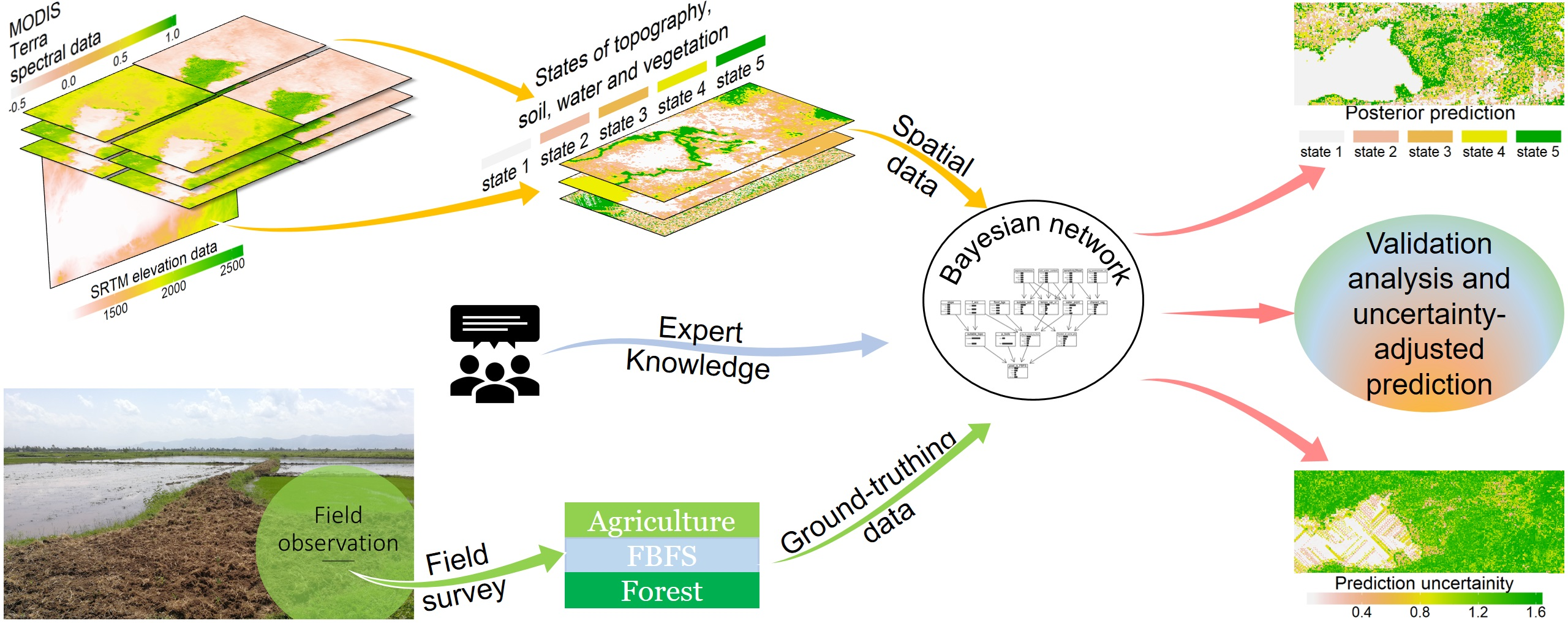
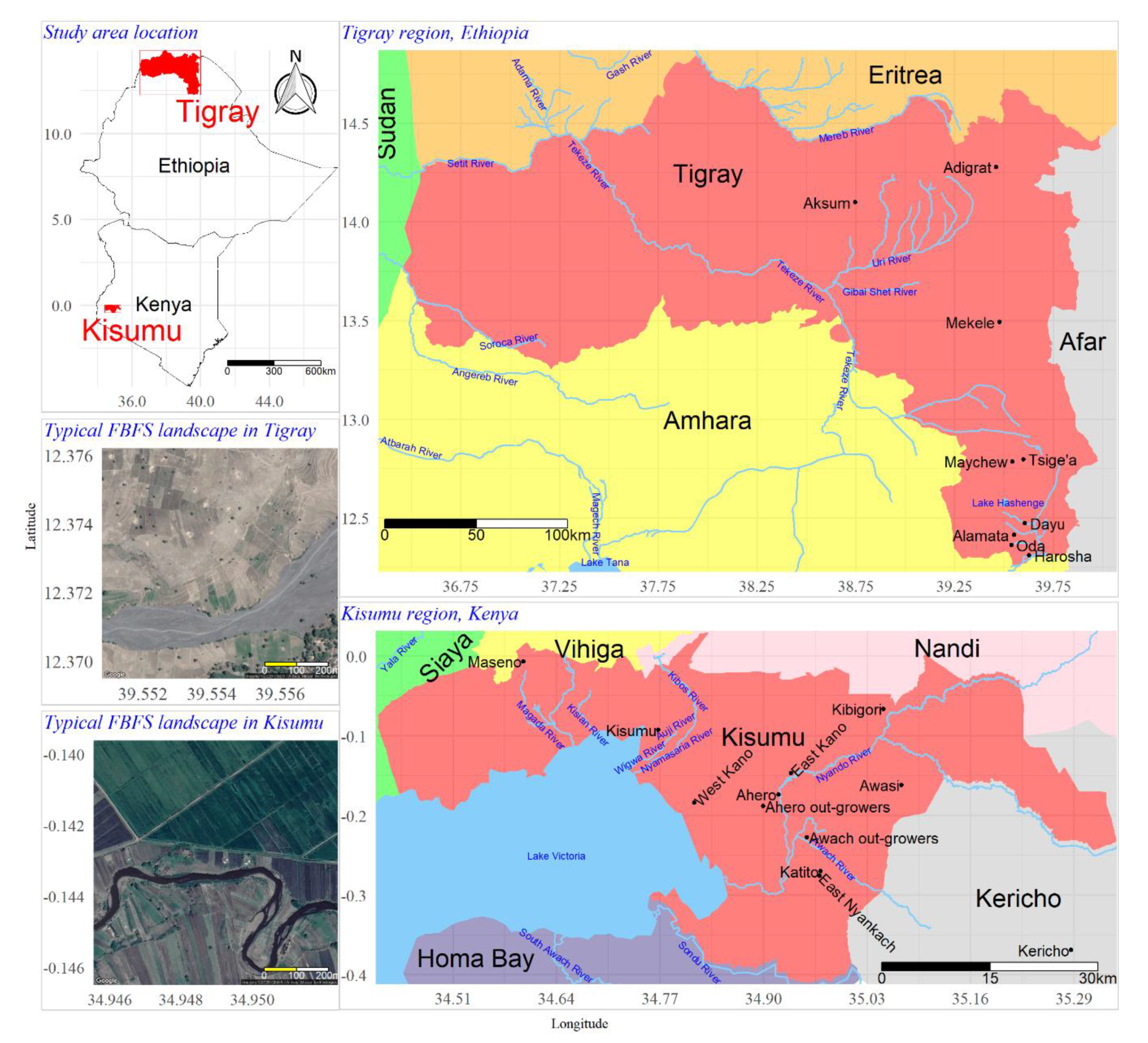
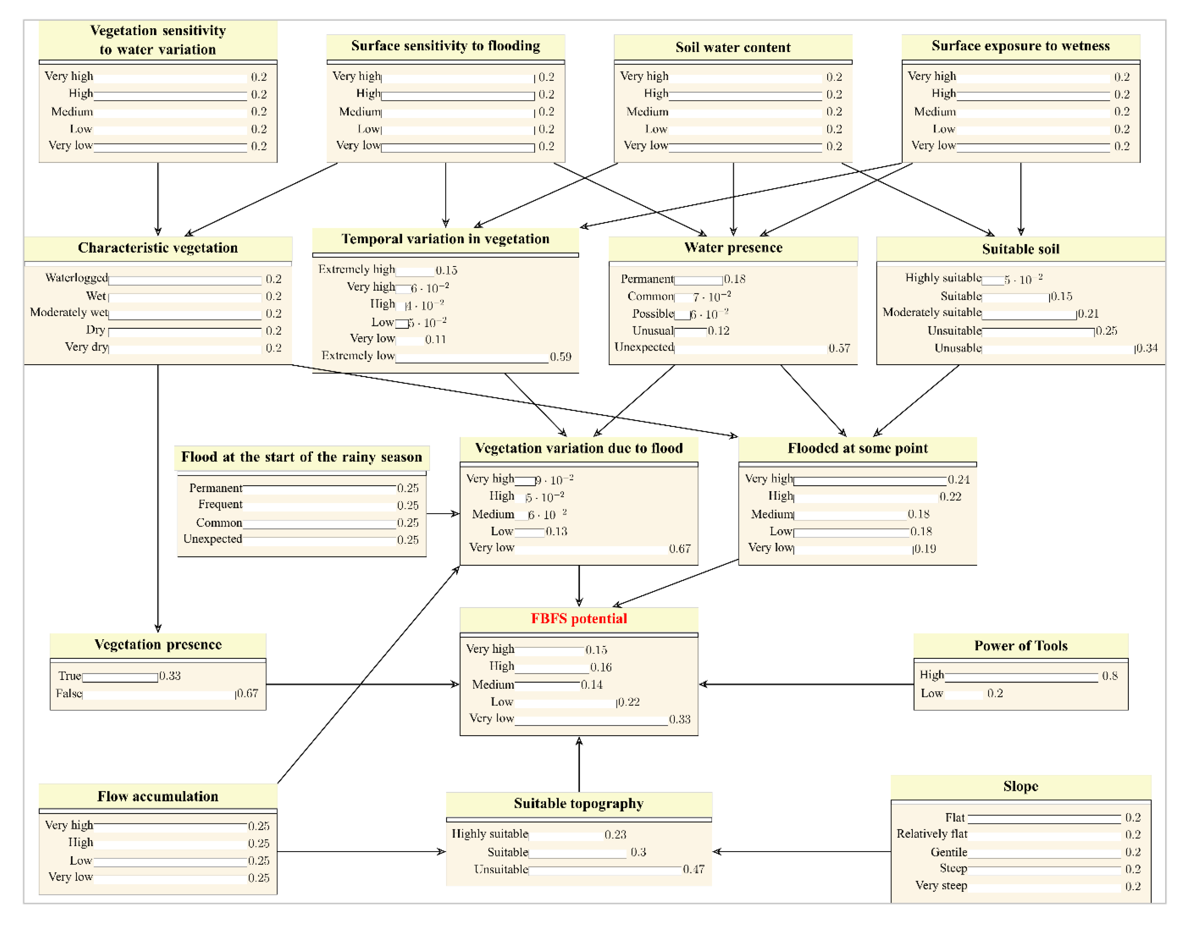
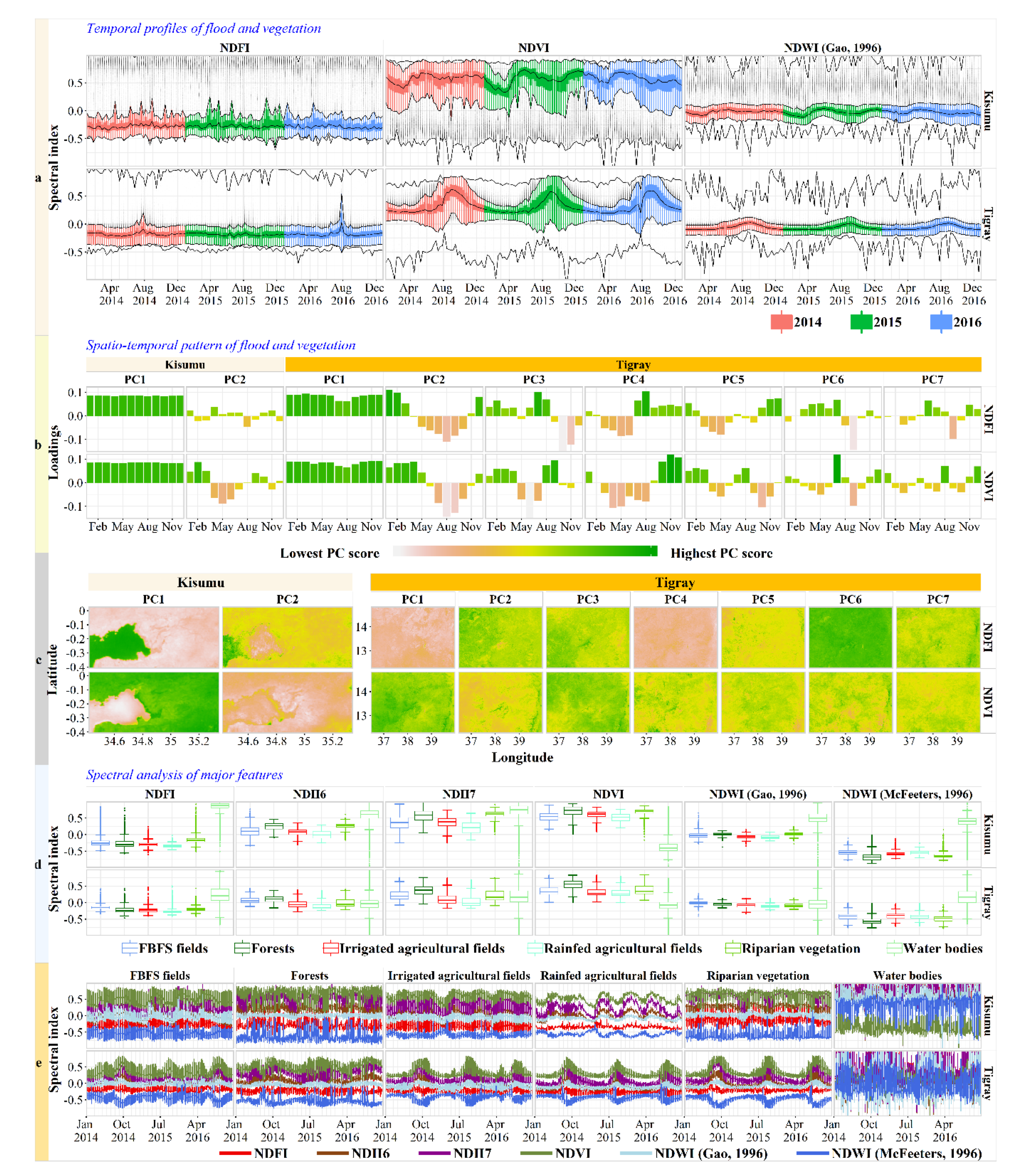
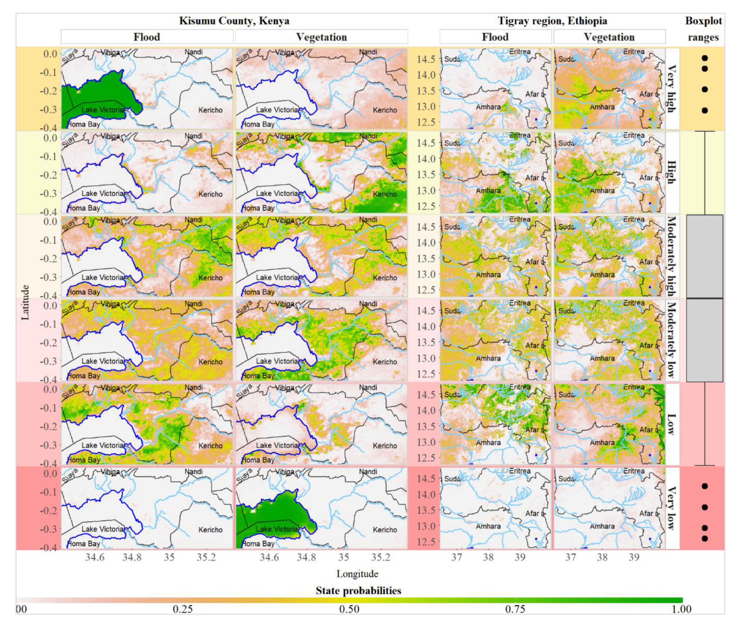
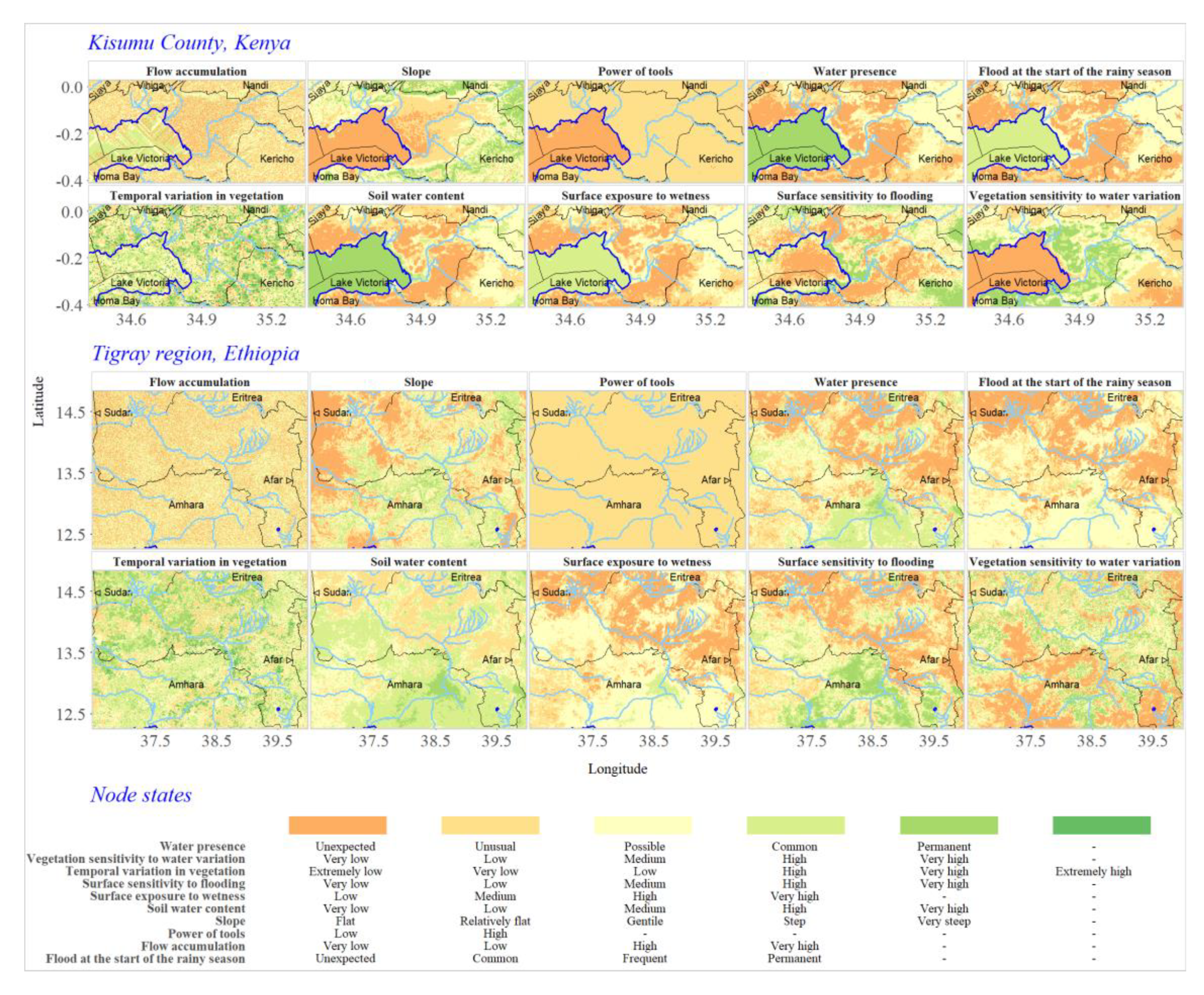
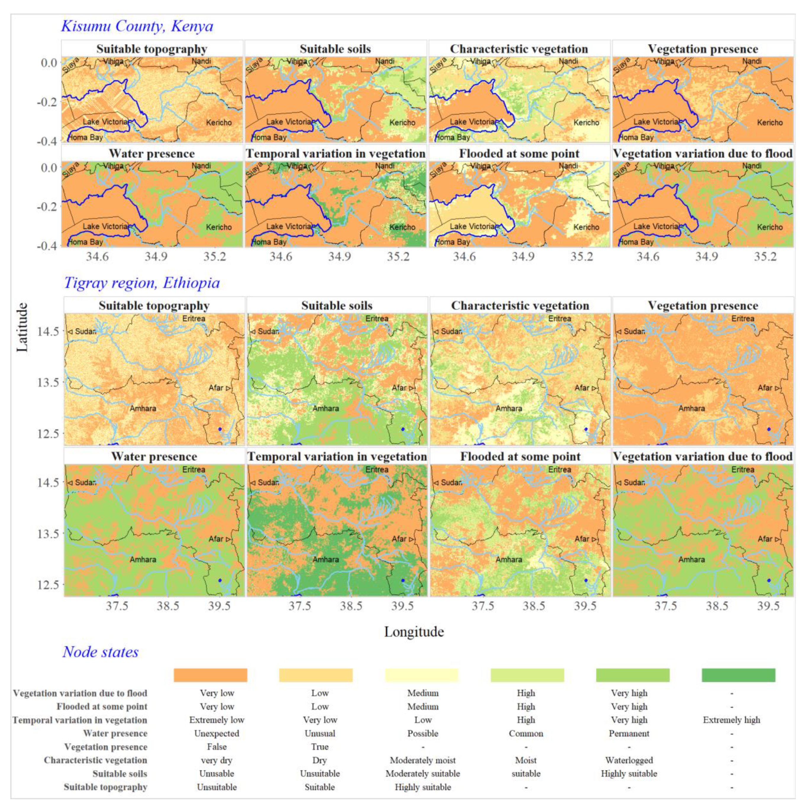
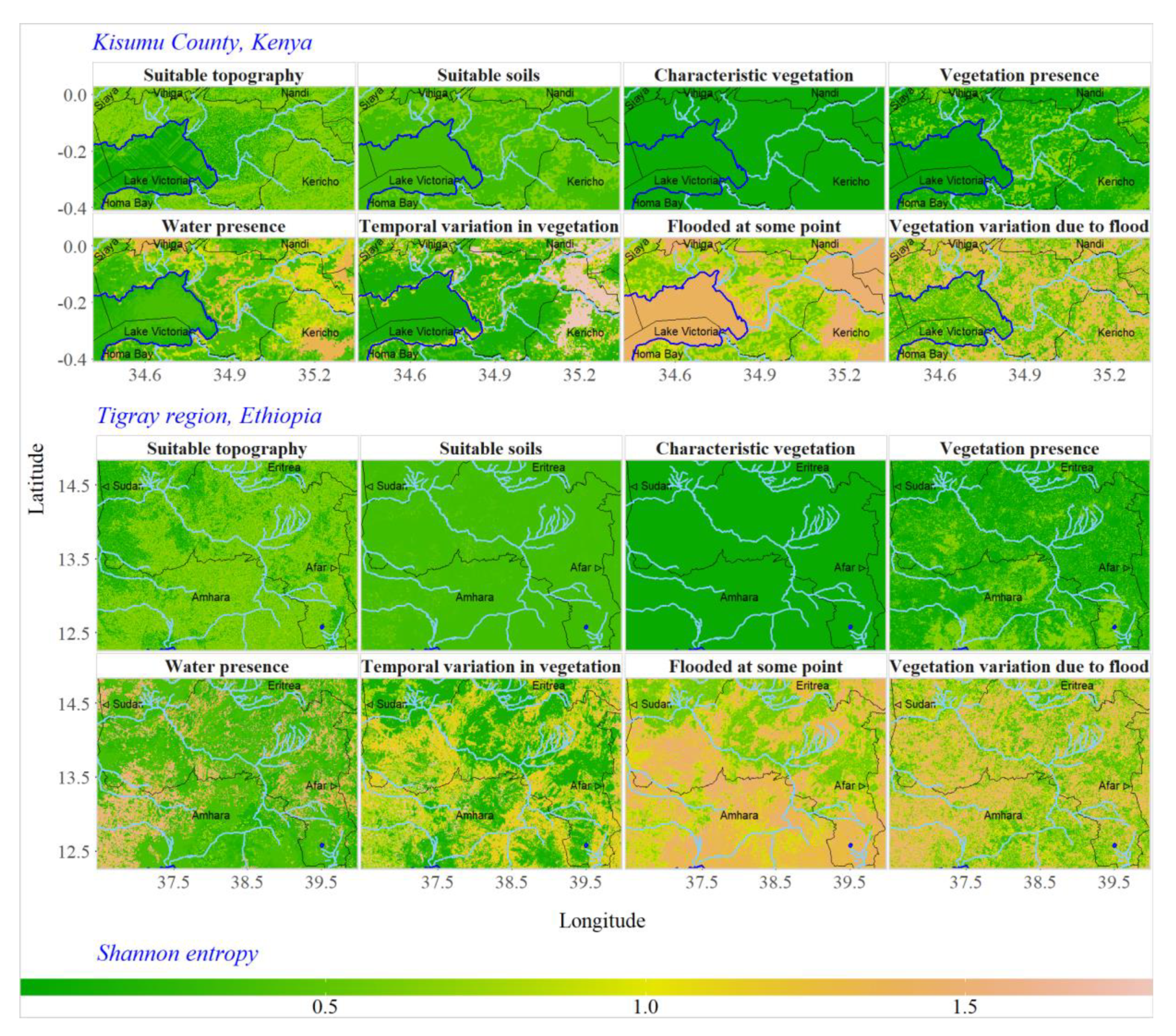
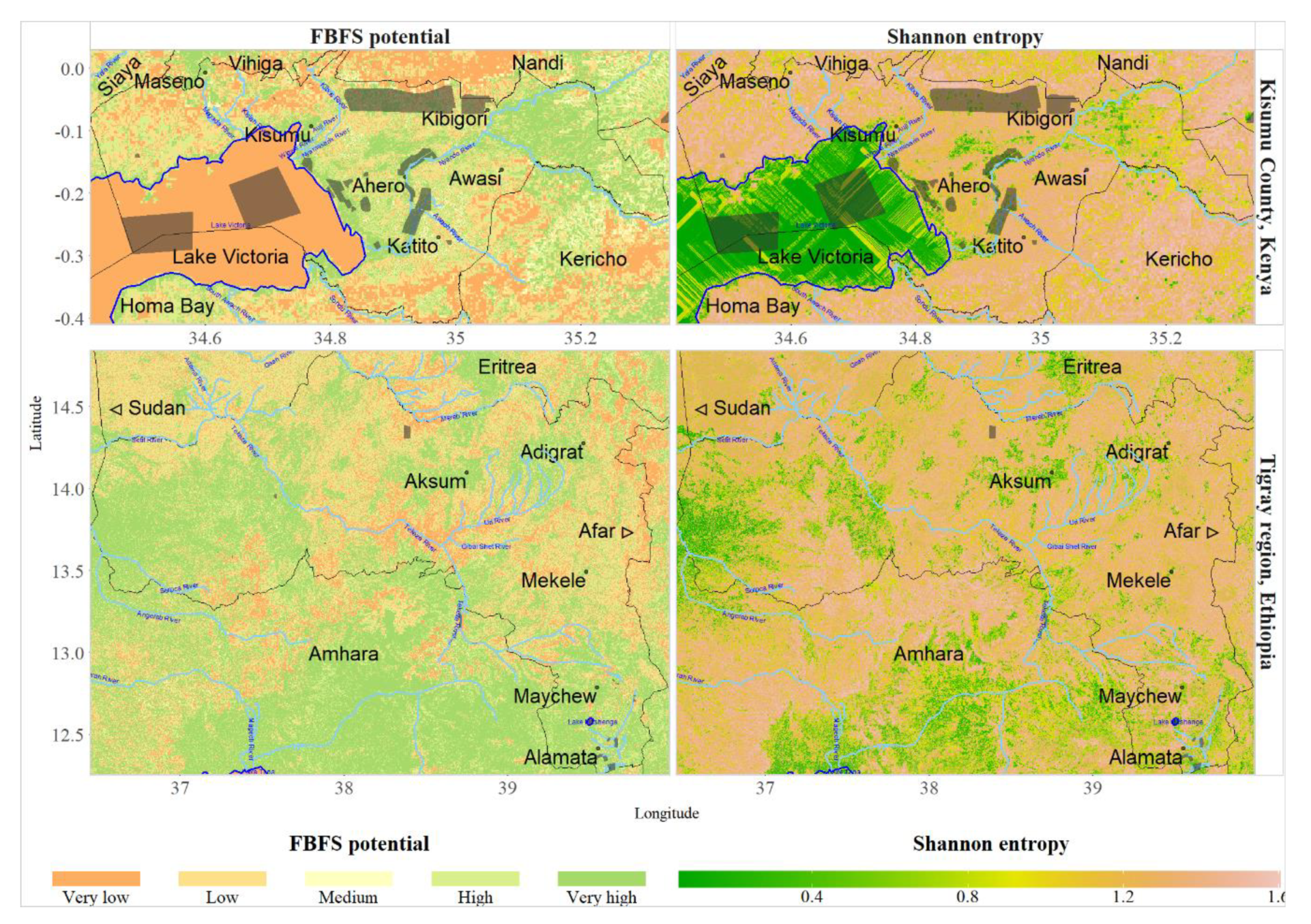
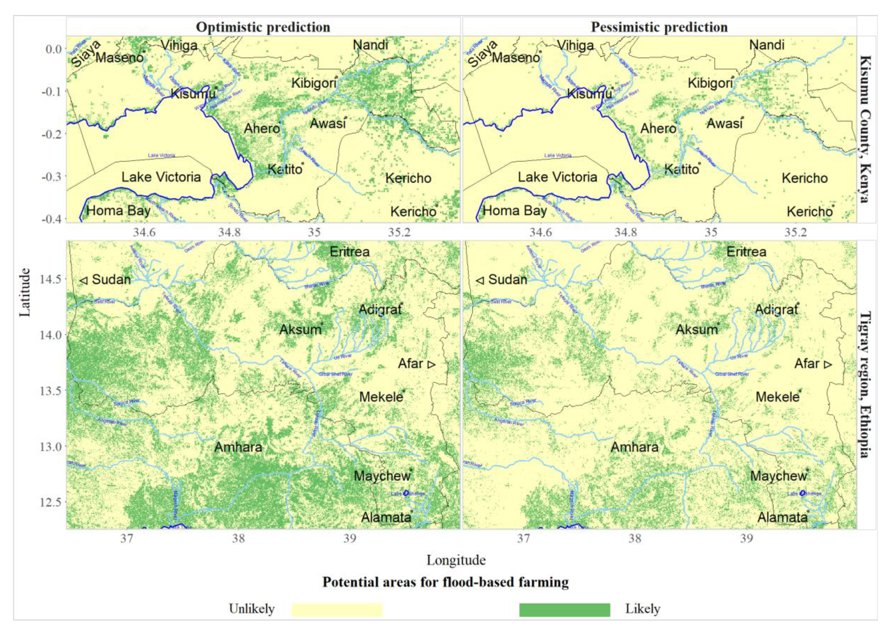
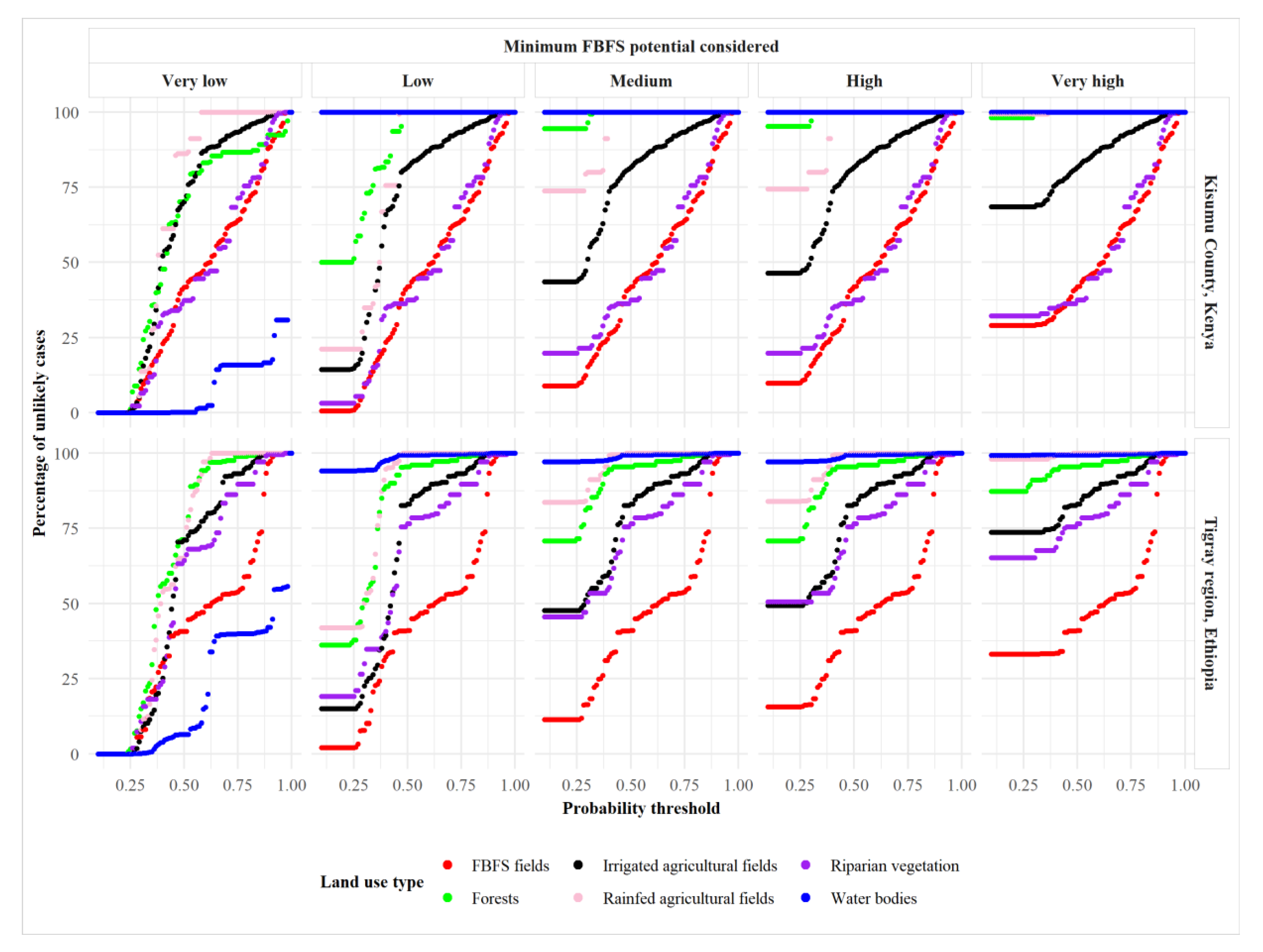
Table 1.
List of normalized difference spectral indices used to estimate several spatial data nodes to feed a Bayesian network for mapping FBFS in Kisumu County, Kenya, and Tigray region, Ethiopia.
Table 1.
List of normalized difference spectral indices used to estimate several spatial data nodes to feed a Bayesian network for mapping FBFS in Kisumu County, Kenya, and Tigray region, Ethiopia.
| Spectral Index | MODIS Bands | MODIS Spectral Range | Full Name |
|---|---|---|---|
| NDVI | B2, B1 | (NIR2 − VISRed)/(NIR + VISRed) | Normalized Difference Vegetation Index [10] |
| NDFI | B1, B6 | (NIR1 − SWIR1)/(NIR + SWIR1) | Normalized Difference Flood Index [17] |
| NDII6 | B2, B6 | (NIR2 − SWIR1)/(NIR2 + SWIR1) | Normalized Difference Infrared Index—Band 6 [11] |
| NDII7 | B2, B7 | (NIR2 − SWIR2)/(NIR2 + SWIR2) | Normalized Difference Infrared Index—Band 7 [11] |
| Gao NDWI | B2, B5 | (NIR2 − NIR5)/(NIR2 + NIR5) | Normalized Difference Water Index (NDWI) [12] |
| McFeeters NDWI | B4, B2 | (VISgreen − NIR2)/(VISgreen + NIR2) | Normalized Difference Water Index (NDWI) [13] |
Table 2.
Translation of 2-bit pixel level quality assessment in MODLAND [48] used to estimate pixel data quality.
Table 2.
Translation of 2-bit pixel level quality assessment in MODLAND [48] used to estimate pixel data quality.
| 2-Bit Encoded per Pixel QA Code | Decimal Value | Quality Attribute Meaning |
|---|---|---|
| 00 | 0 | Pixel produced, good quality, not necessary to examine more detailed QA |
| 01 | 1 | Pixel produced, unreliable or unquantifiable quality, recommend examination of more detailed QA |
| 10 | 2 | Pixel not produced due to cloud effects |
| 11 | 3 | Pixel not produced primarily due to reasons other than cloud |
Table 3.
Description of data used to validate a Bayesian network mapping procedure for FBFS in Kisumu County, Kenya, and Tigray region, Ethiopia.
Table 3.
Description of data used to validate a Bayesian network mapping procedure for FBFS in Kisumu County, Kenya, and Tigray region, Ethiopia.
| Study Area | Validation Polygons | |||
|---|---|---|---|---|
| Land Use Type | Description | Number | Area (km2) | |
| Kisumu | FBFS fields | Water is mainly acquired via gravity from rivers or lakes | 11 | 48.9 |
| Forests | More than 60% tree cover | 5 | 7.3 | |
| Irrigated agricultural fields | Water is mainly acquired using pumps | 2 | 92.0 | |
| Rainfed agricultural fields | Water mainly acquired via rainfall | 2 | 1.3 | |
| Riparian vegetation | Vegetation close to water | 4 | 6.7 | |
| Water bodies | Areas permanently covered by water | 2 | 164.9 | |
| Tigray | FBFS fields | Water is mainly acquired via gravity from dry wadis | 9 | 65.7 |
| Forests | More than 60% tree cover | 4 | 3.3 | |
| Irrigated agricultural fields | Water is mainly acquired using pumps and wells | 4 | 9.9 | |
| Rainfed agricultural fields | Water mainly acquired via rainfall | 2 | 38.0 | |
| Riparian vegetation | Vegetation close to water | 4 | 1.6 | |
| Water bodies | Areas permanently covered by water | 5 | 33.2 | |
Table 4.
Spatial coverage of flood-based farming systems (FBFS) in Kisumu County, Kenya and Tigray, Ethiopia derived from a classification algorithm based on an expert-informed Bayesian network.
Table 4.
Spatial coverage of flood-based farming systems (FBFS) in Kisumu County, Kenya and Tigray, Ethiopia derived from a classification algorithm based on an expert-informed Bayesian network.
| Study Area | Area Covered by the Respective FBFS Potential Class (km2 and Share of Total Area) | ||||
|---|---|---|---|---|---|
| Very Low | Low | Medium | High | Very High | |
| Kisumu County, Kenya | 873.3 (32.8%) | 552.7 (20.7%) | 72.5 (2.7%) | 495.5 (18.6%) | 670.8 (25.2%) |
| Tigray region, Ethiopia | 9000.9 (17.1%) | 11,185.2 (21.3%) | 597.0 (1.1%) | 11,530.2 (21.9%) | 20,209.3 (38.5%) |
Table 5.
Accuracy assessment of a map derived from an expert-informed Bayesian network mapping of flood-based farming systems (FBFS) potential in Kisumu County, Kenya and Tigray, Ethiopia.
Table 5.
Accuracy assessment of a map derived from an expert-informed Bayesian network mapping of flood-based farming systems (FBFS) potential in Kisumu County, Kenya and Tigray, Ethiopia.
| Study Area | Validation Polygons | FBFS Potential | ||||||
| Land use type | Number | Area (km2) | Very low | Low | Medium | High | Very high | |
| Kisumu | FBFS fields | 11 | 48.9 | 0.6% | 8.4% | 0.9% | 19.2% | 70.9% |
| Forests | 5 | 7.3 | 50.0% | 44.6% | 0.6% | 2.8% | 1.9% | |
| Irrigated agricultural fields | 2 | 92.0 | 14.4% | 29.1% | 2.9% | 22.1% | 31.5% | |
| Rainfed agricultural fields | 2 | 1.3 | 21.3% | 52.5% | 0.6% | 25.0% | 0.6% | |
| Riparian vegetation | 4 | 6.7 | 3.2% | 16.5% | 0.0% | 12.4% | 67.8% | |
| Water bodies | 2 | 164.9 | 100.0% | 0.0% | 0.0% | 0.0% | 0.0% | |
| Tigray | FBFS fields | 9 | 65.7 | 2.1% | 9.2% | 4.3% | 17.5% | 66.8% |
| Forests | 4 | 3.3 | 36.1% | 34.7% | 0.0% | 16.5% | 12.7% | |
| Irrigated agricultural fields | 4 | 9.9 | 15.0% | 32.7% | 1.7% | 24.3% | 26.3% | |
| Rainfed agricultural fields | 2 | 38.0 | 41.9% | 41.7% | 0.4% | 14.0% | 2.0% | |
| Riparian vegetation | 4 | 1.6 | 19.1% | 26.5% | 4.9% | 14.7% | 34.8% | |
| Water bodies | 5 | 33.2 | 94.0% | 3.1% | 0.0% | 2.2% | 0.7% | |
© 2020 by the authors. Licensee MDPI, Basel, Switzerland. This article is an open access article distributed under the terms and conditions of the Creative Commons Attribution (CC BY) license (http://creativecommons.org/licenses/by/4.0/).
Share and Cite
MDPI and ACS Style
Liman Harou, I.; Whitney, C.; Kung’u, J.; Luedeling, E. Mapping Flood-Based Farming Systems with Bayesian Networks. Land 2020, 9, 369. https://doi.org/10.3390/land9100369
AMA Style
Liman Harou I, Whitney C, Kung’u J, Luedeling E. Mapping Flood-Based Farming Systems with Bayesian Networks. Land. 2020; 9(10):369. https://doi.org/10.3390/land9100369
Chicago/Turabian StyleLiman Harou, Issoufou, Cory Whitney, James Kung’u, and Eike Luedeling. 2020. "Mapping Flood-Based Farming Systems with Bayesian Networks" Land 9, no. 10: 369. https://doi.org/10.3390/land9100369
Note that from the first issue of 2016, this journal uses article numbers instead of page numbers. See further details here.