
Modelling the Potential of Integrated Vegetation Bands (IVB) to Retain Stormwater Runoff on Steep Hillslopes of Southeast Queensland, Australia


Abstract
:
1. Introduction
2. Method
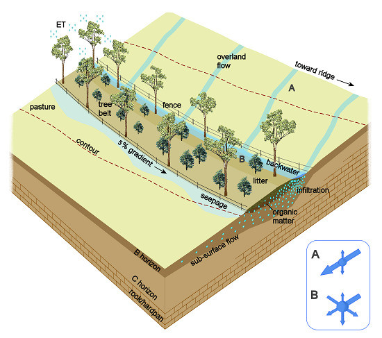
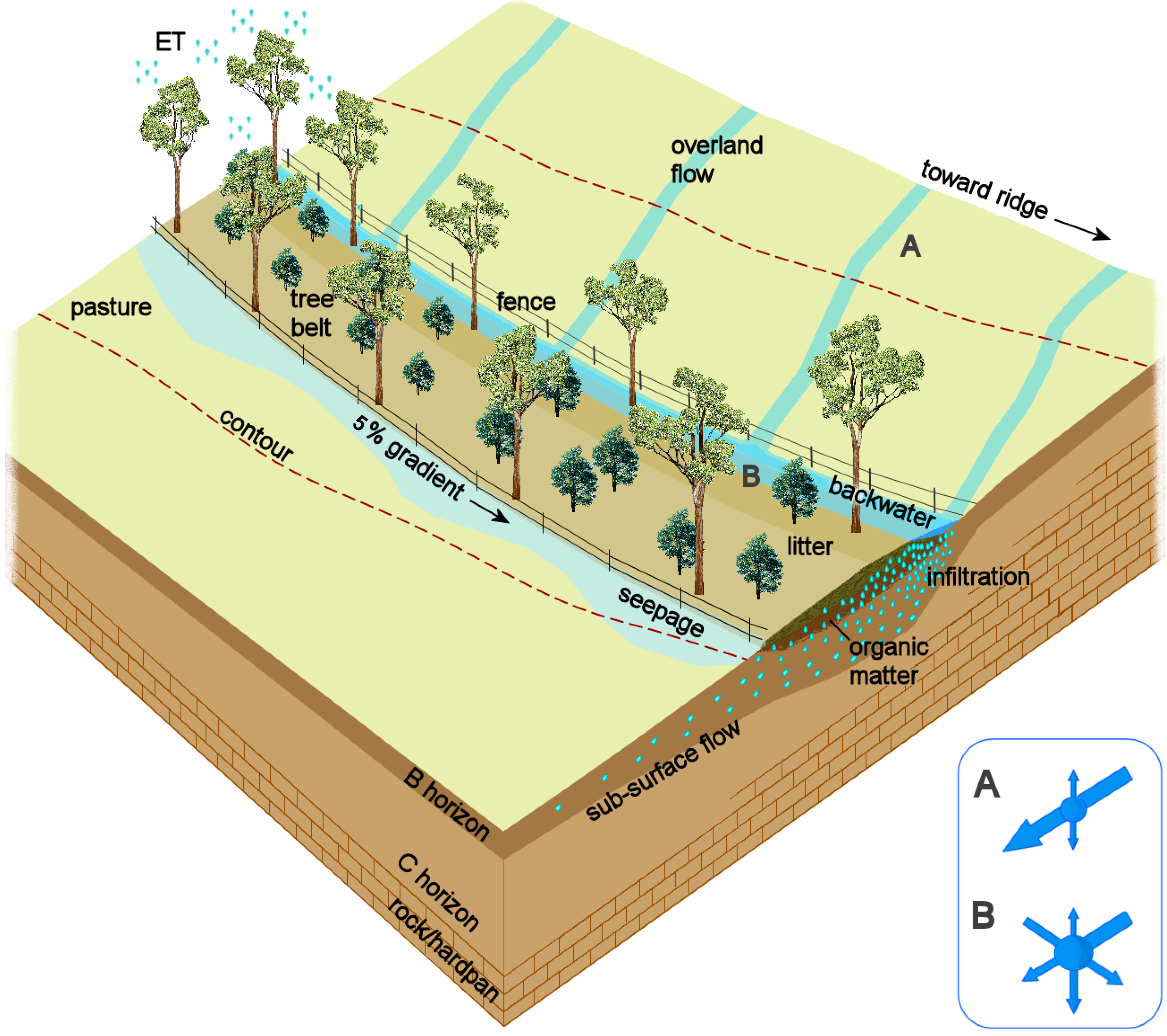
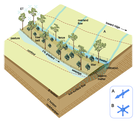
2.1. Conceptual Model
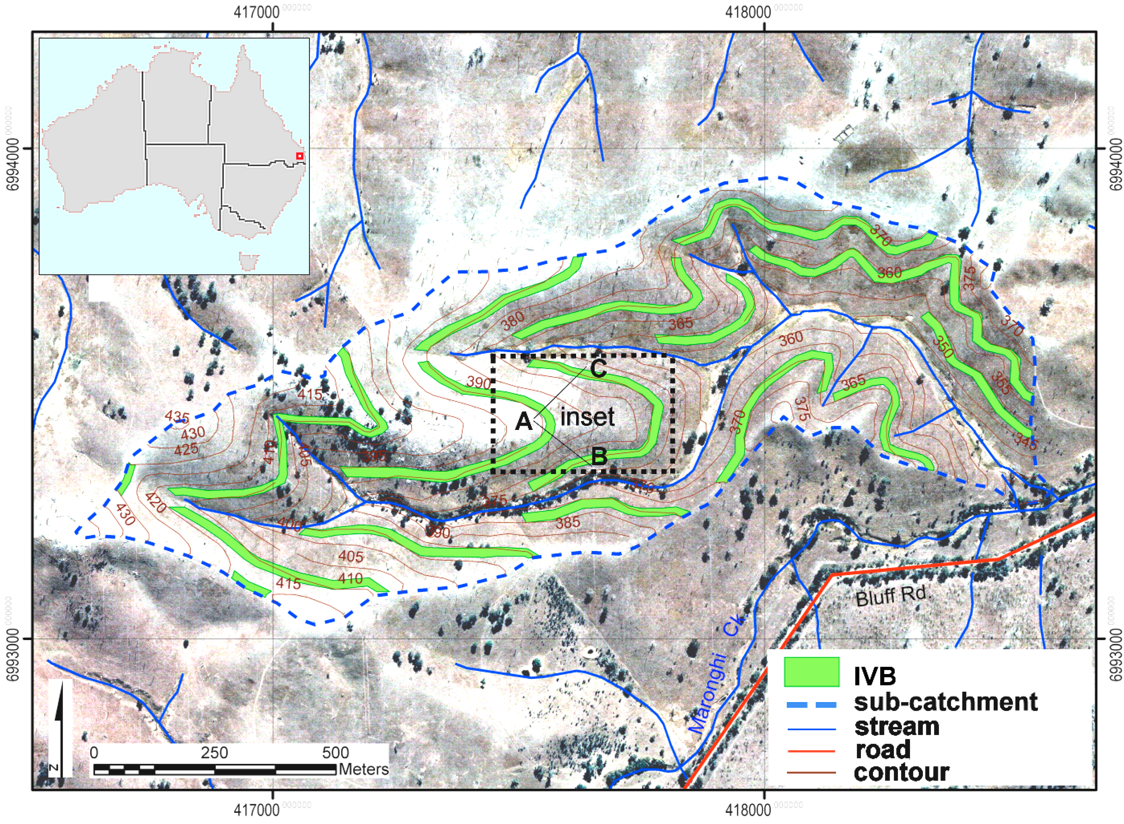
2.2. Study Area
2.3. Software
2.4. Data Compilation and Parameter Estimates

| Variable | Pasture | IVB |
|---|---|---|
| Topography | 10 m DEM | 10 m DEM |
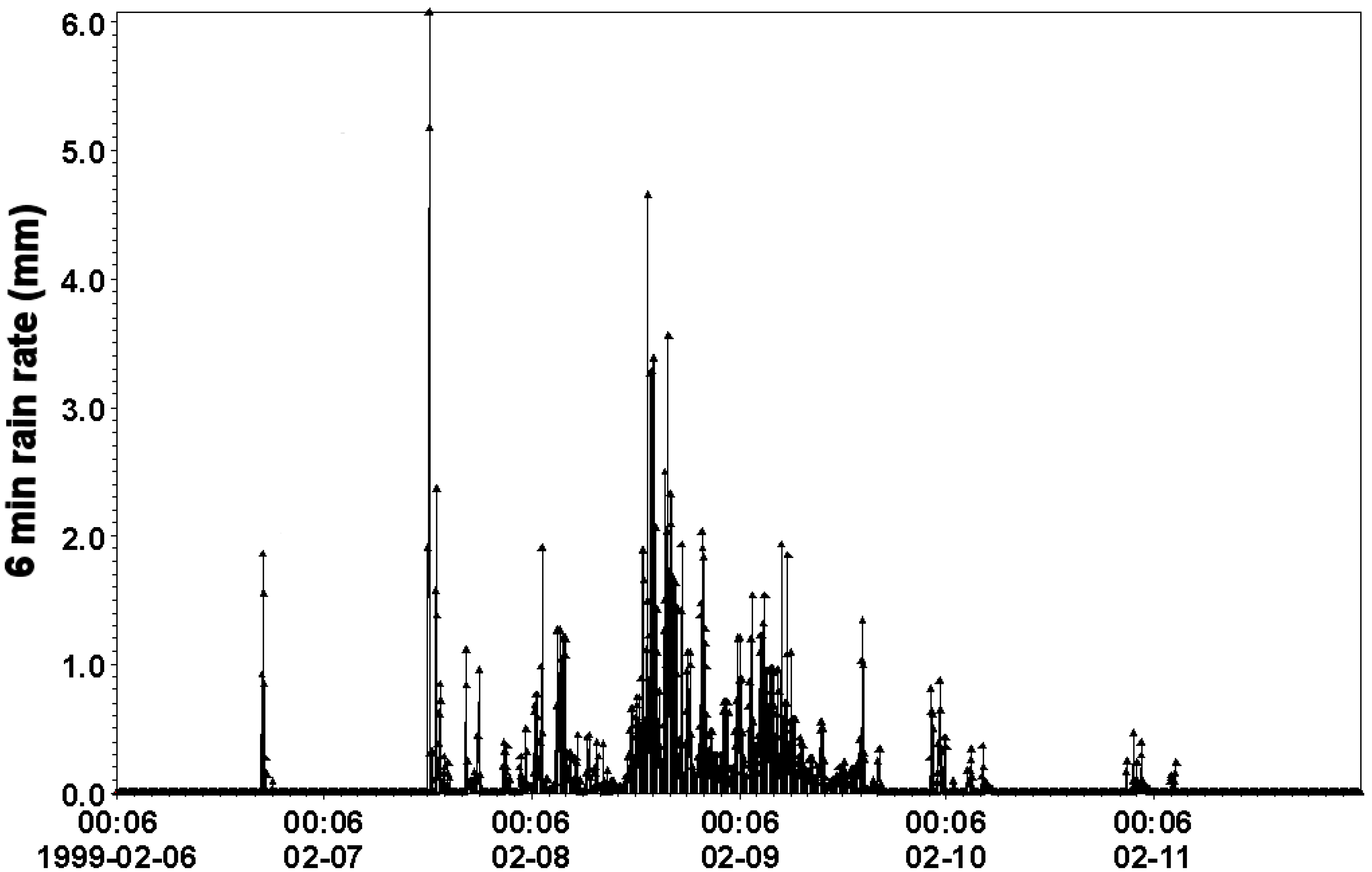
| Pluviograph a | 6 min | 6 min |
| Reference evapotranspiration (mm/day) b,c | 1.6 | 2.6 |
| Reference evaporation (mm/day) b,c | 7 | 7 |
| Leaf Area Index b,g | 0.5 | 2 |
| Rooting depth (m) j | 0.3 | 0.9 |
| Soil depth | 0.3 * | 0.65 |
| Soil type j | Orthic Tenosol | Orthic Tenosol |
| Infiltration rate (mm/h) j | 14 | 19 |
| Water content (saturation) h | 0.24 | 0.38 |
| Water content (field) h | 0.16 | 0.16 |
| Water content (wilting) h | 0.10 | 0.10 |
| Saturated hydraulic conductivity (m/s) f | 9.75 × 10⁻⁶ | 9.75 × 10⁻⁶ |
| Vertical hydraulic conductivity (m/s)f | 1.6 × 10⁻⁸ | 1.6 × 10⁻⁸ |
| Surface roughness (m2(1/3)/s2) d,e,i (Manning’s M) | 12.5 | 2.5 |
| Detention storage (mm) | 3 | 8 |
| Specific yield (mm) f | 0.2 | 0.2 |
| Specific storage (mm) f | 0.02 | 0.02 |

3. Results
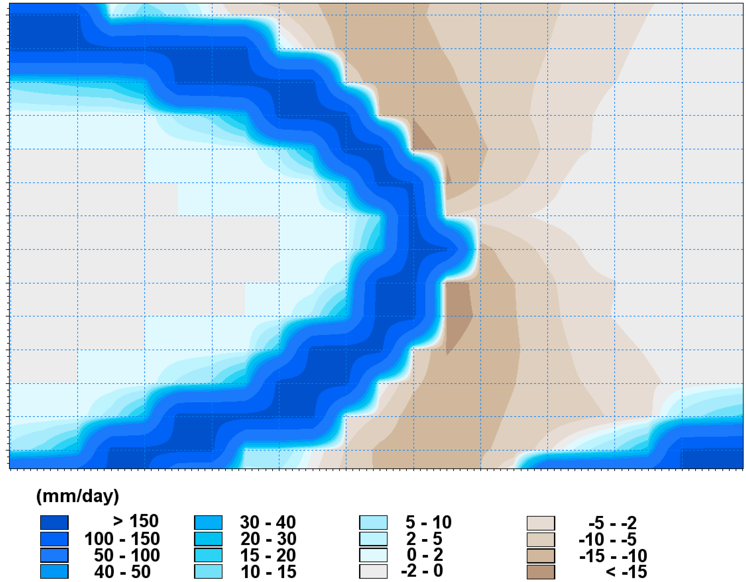
3.1. Spatial Distribution of Overland Flow and Infiltration
3.1.1. Hillslope Scale


3.1.2. Sub-Catchment Scale

| Mean (OFµ) | Max (OFmax) | ||||||
|---|---|---|---|---|---|---|---|
| Area | Day | Pasture | IVB | Δ% | Pasture | IVB | Δ% |
| sub-catchment | 1 | 0.008 | 0.008 | −2 | 0.370 | 0.257 | −31 |
| 2 | 0.010 | 0.007 | −28 | 0.672 | 0.517 | −23 | |
| 3 | 0.023 | 0.024 | +2 | 1.809 | 1.774 | −2 | |
| 4 | 0.002 | 0.002 | −64 | 0.216 | 0.216 | +0.2 | |
| 5 | <0.001 | <0.001 | +60 | 0.212 | 0.212 | 0 | |
| hillslope (subset) | 1 | 0.007 | 0.007 | +12 | 0.012 | 0.020 | +64 |
| 2 | 0.004 | 0.004 | −2 | 0.007 | 0.013 | +101 | |
| 3 | 0.004 | 0.005 | +28 | 0.005 | 0.011 | +121 | |
| 4 | 0.001 | 0.002 | +94 | 0.002 | 0.007 | +246 | |
| 5 | <0.001 | <0.001 | * | 0.001 | 0.005 | +287 | |
3.2. Model Water Balance Predictions
| Pasture | IVB | |||||||
|---|---|---|---|---|---|---|---|---|
| Variable | Min | Max | Mean | S.E. | Min | Max | Mean | S.E. |
| Net Precipitation | 276 | 276 | ||||||
| Evaporation | 0 | 23 | 8 | 0.22 | 0 | 23 | 8 | 0.22 |
| Infiltration | 0 | 54 | 38 | 0.57 | 0 | 66 | 46 | 0.71 |
| SZ- > OF | −5 | 0 | −2 | 0.04 | −5 | 0 | −2 | 0.04 |
| OF- > SZ | 0 | 2 | 1 | 0.02 | 0 | 2 | 1 | 0.02 |
| Q | 0 | 211 | 98 | 2.55 | 0 | 197 | 90 | 2.39 |
| OF Stor.Change | 0 | 42 | 8 | 0.34 | 0 | 42 | 8 | 0.34 |
| Error | −33 | 10 | −0.2 | 0.30 | −30 | 9 | −0.3 | 0.27 |
3.3. Model Sensitivity Analysis
3.3.1. Soil Water Content at Saturation (SAT)
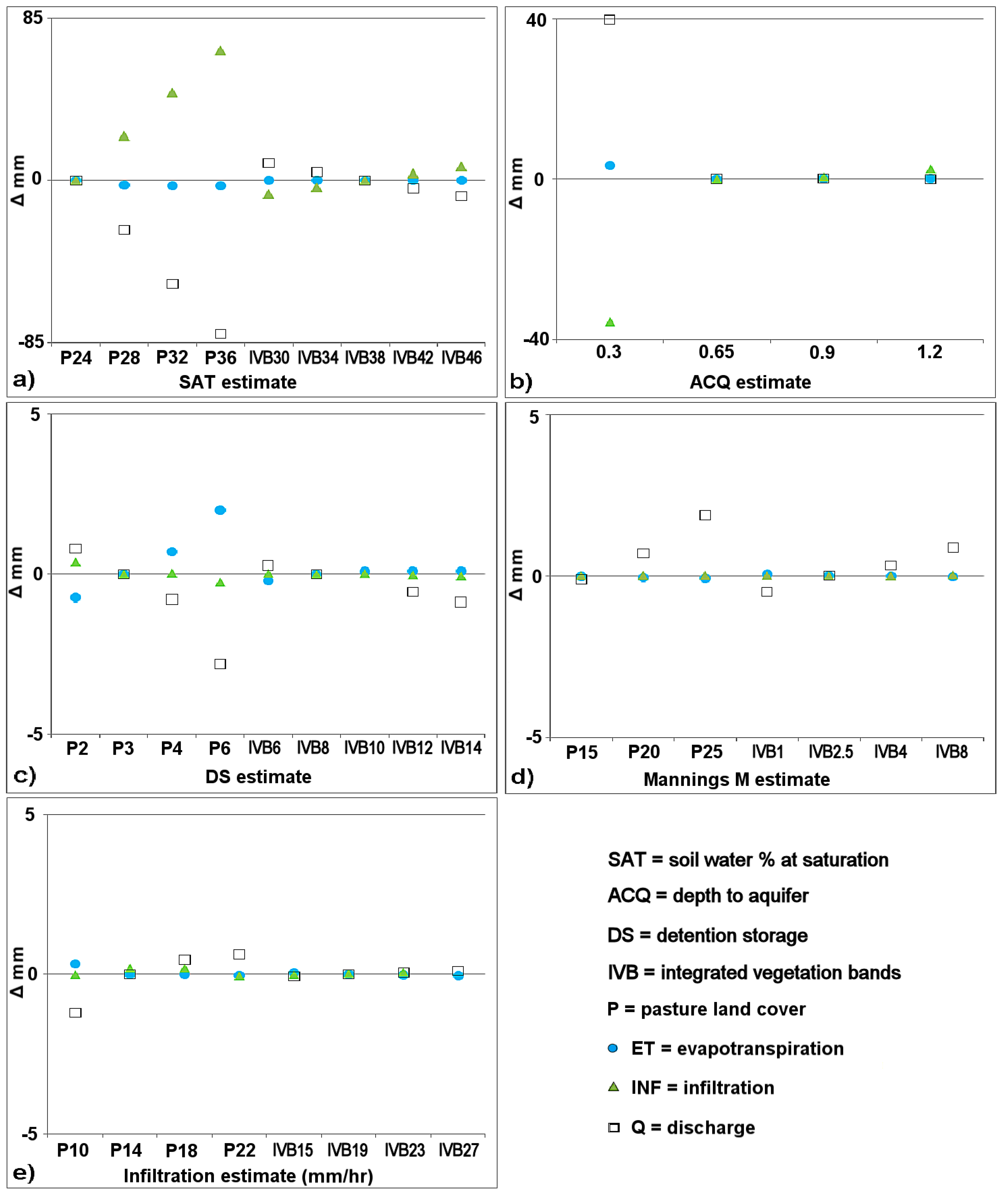
3.3.2. Soil Depth (ACQ)
3.3.3. Detention Storage (DS)
3.3.4. Surface Roughness (M)
3.3.5. Hydraulic Conductivity of Surface Soil (Ks)
4. Discussion
4.1. Major Findings and Comparisons to Other Vegetation Systems
4.2. Model Performance
4.2.1. Saturated Soil Water Content (SAT)
4.2.2. Depth to Impermeable Layer (ACQ)
4.2.3. Detention Storage
4.2.4. Surface Roughness (Manning’s M)
4.2.5. Saturated Hydraulic Conductivity (Ks)
4.3. Management Implications
4.3.1. Benefits of IVB
4.3.2. Limitations of IVB
4.4. Research Limitations and Questions
5. Conclusions
- •
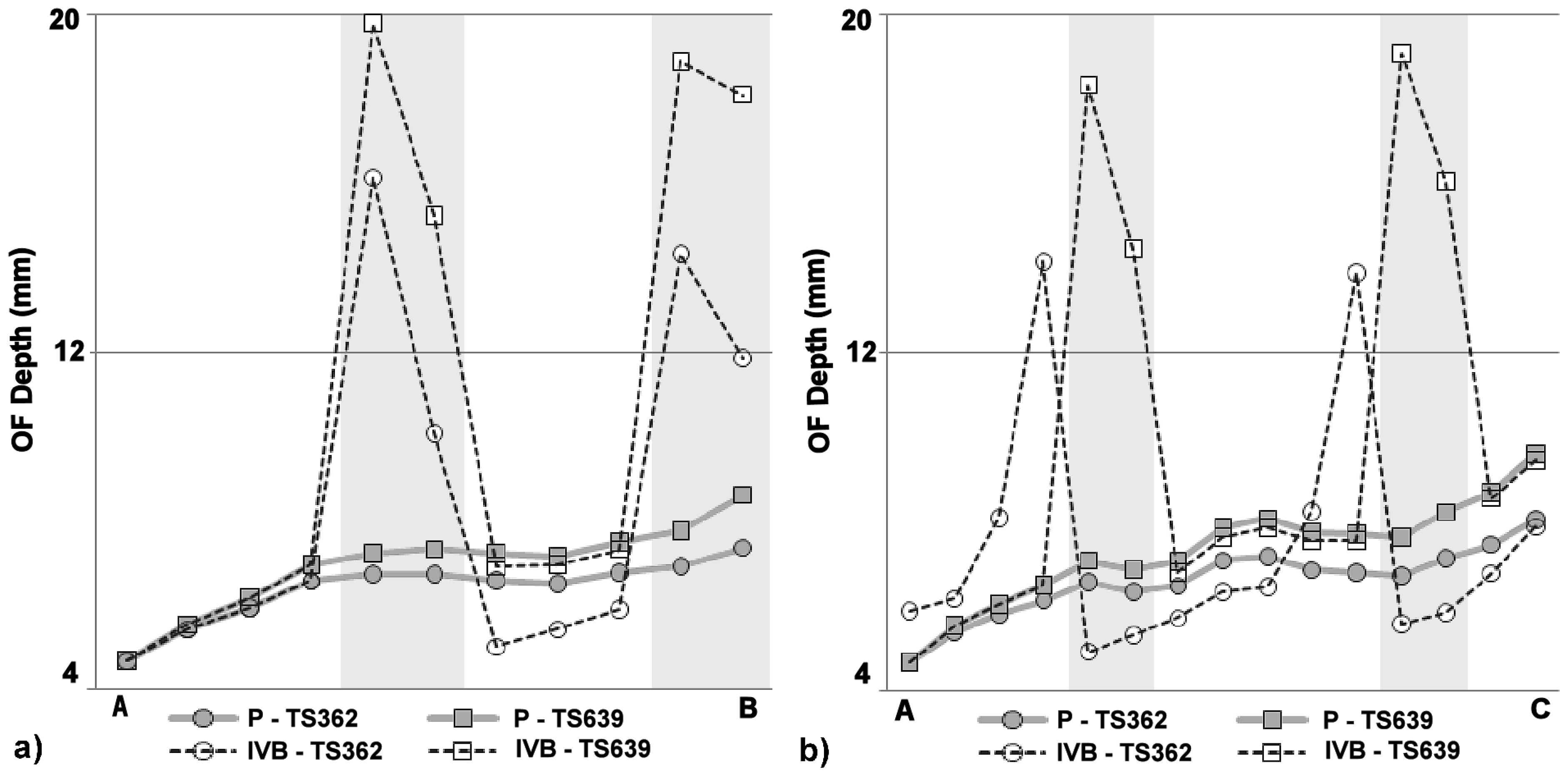
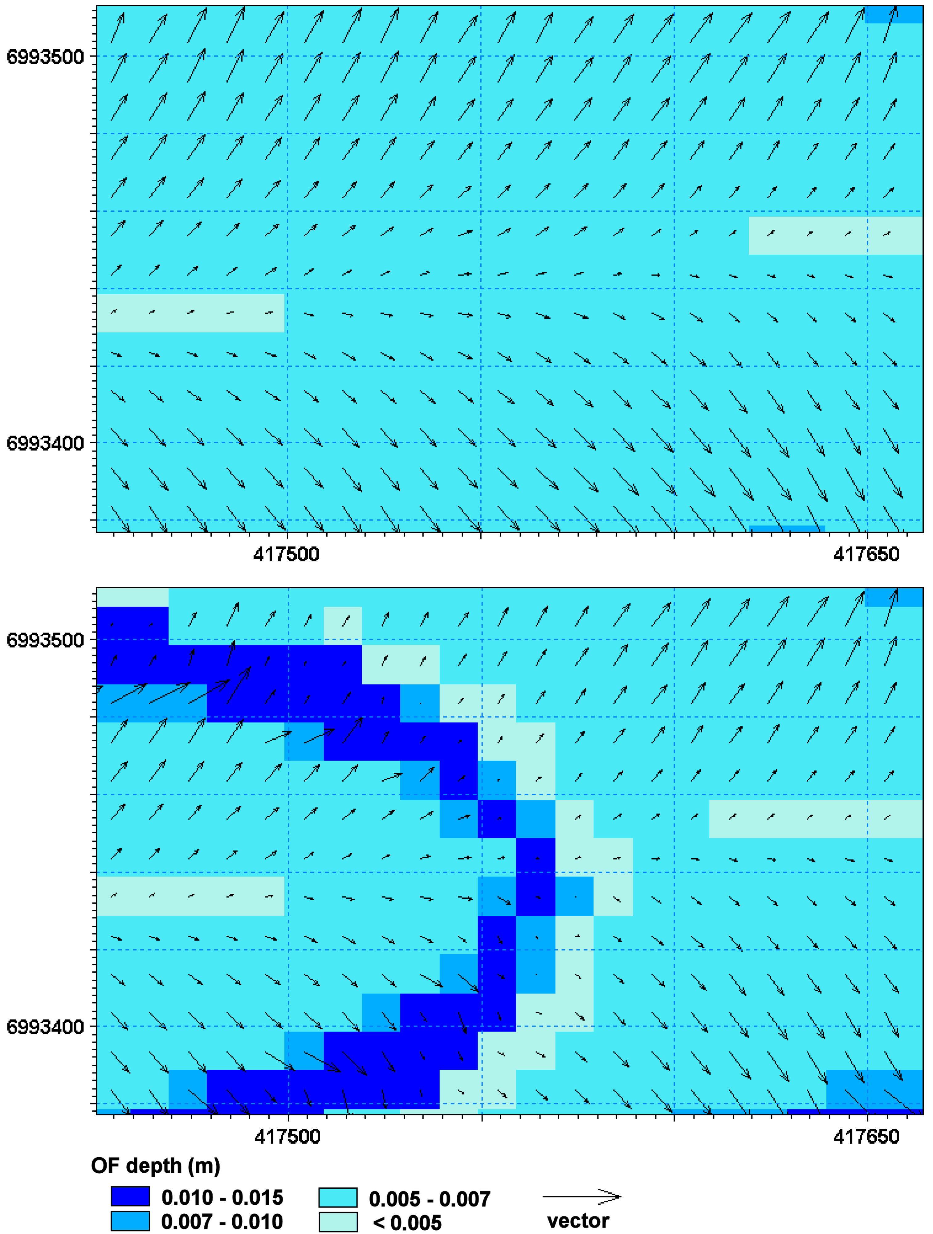
- At the hillslope scale, simulations predicted that water depth increased beneath IVB but decreased in inter-band spaces. The actual area of hillslope where more than 10 mm of runoff was retained was increased by 22% in IVB compared to the pasture land cover, or an 11% increase in hillslope area external to IVB where extra runoff was retained.
- •
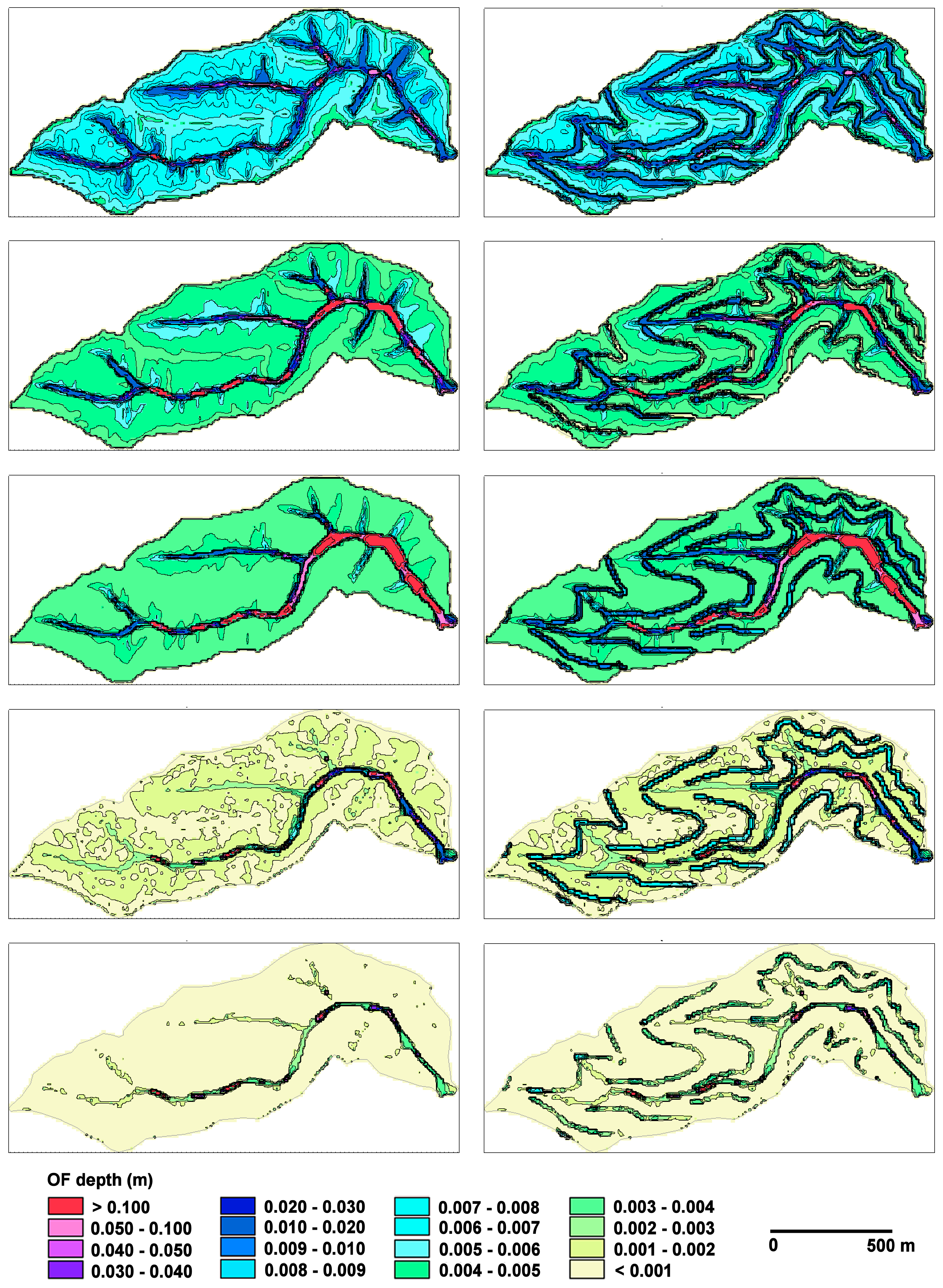
- At the sub-catchment scale, simulations predicted that landscapes with IVB would have 23% more infiltration and 7% less discharge than landscapes without these bands. There was a slight lengthening of base flow in the channel.
- •
- Higher SAT levels and greater soil depth were the primary drivers for differences in ecohydrological functioning between pasture and IVB, with secondary functional differences including increased surface roughness, detention storage and infiltration rate.
- •
- Information on the effects of each parameter was used to optimise the selection of instrumentation for a current paired catchment field trial in Southeast Queensland. The findings may also serve as a guide for establishing similar adaptations of IVB in other regions where protection of hillslopes and catchment systems against greater rainfall intensity may be required.
Acknowledgments
Author Contributions
Conflicts of Interest
References
- Falkenmark, M.; Rockstrom, J. Balancing Water for Humans and Nature: The New Approach in Ecohydrology; Earthscan Publications: London, UK, 2004. [Google Scholar]
- Muller, C.; Malone, T. The Southeast Queensland Flash Flood Event of 9 March 2001; Bureau of Meteorology: Brisbane, QLD, Australia, 2001; p. 54.
- Pachauri, R.K.; Reisinger, A. Climate Change 2007: Synthesis Report. Contribution of Working Groups I, II and III to the Fourth Assessment Report of the Intergovernmental Panel on Climate Change; IPCC: Geneva, Switzerland, 2007. [Google Scholar]
- Abbs, D.; Rafter, T. Climate change and its impact on extreme rainfall in SE Australia. In High Resolution Modelling: Extended Abstracts of the Second CAWCR Modelling Workshop, 25–28 November 2008; Hollis, A.J., Ed.; Centre for Australian Weather and Climate Research: Melbourne, VIC, Australia, 2008; pp. 33–36. [Google Scholar]
- Gutiérrez-Jurado, H.A.; Vivoni, E.R.; Harrison, J.B.J.; Guan, H.J. Ecohydrology of root zone water fluxes and soil development in complex semiarid rangelands. Hydrol. Process. 2006, 20, 3289–3316. [Google Scholar] [CrossRef]
- Boer, M.; Puigdefabregas, J. Effects of spatially structured vegetation patterns on hillslope erosion in a semiarid Mediterranean environment: A simulation study. Earth Surf. Process. Landf. 2005, 30, 149–167. [Google Scholar] [CrossRef]
- Mitchell, P.B.; Humphreys, G.S. Litter dams and microterraces formed on hillslopes subject to rainwash in the Sydney Basin, Australia. Geoderma 1987, 39, 331–357. [Google Scholar] [CrossRef]
- Dunkerley, D. Surface tension and friction coefficients in shallow, laminar overland flows through organic litter. Earth Surf. Process. Landf. 2002, 27, 45–58. [Google Scholar] [CrossRef]
- Duran Zuazo, V.H.; Martinez, J.R.F.; Pleguezuelo, C.R.R.; Martinez Raya, A.; Rodriguez, B.C. Soil-erosion and runoff prevention by plant covers in a mountainous area (SE Spain): Implications for sustainable agriculture. Environmentalist 2006, 26, 309–319. [Google Scholar] [CrossRef]
- Leguedois, S.; Ellis, T.W.; Hairsine, P.B.; Tongway, D.J. Sediment trapping by a tree belt: processes and consequences for sediment delivery. Hydrol. Process. 2008, 22, 3523–3534. [Google Scholar] [CrossRef]
- Blanco-Canqui, H.; Gantzer, C.J.; Anderson, S.H. Performance of grass barriers and filter strips under interrill and concentrated flow. J. Environ. Qual. 2006, 35, 1969–1974. [Google Scholar] [CrossRef] [PubMed]
- Wilson, B.; Lemon, J. Scattered native trees and soils heterogeneity in grazing land on the northern Tablelands of NSW. In Proceedings of the SuperSoil 2004—3rd Australian New Zealand Soils Conference, Sydney, NSW, Australia, 5–9 December 2004.
- Rao, L.; Zhu, J. Hydrological effects of forest litter and soil in the Simianshan Mountains in Chonging, China. Front. For. China 2007, 2, 157–162. [Google Scholar] [CrossRef]
- Rachman, A.; Anderson, S.H.; Gantzer, C.J.; Thompson, A.L. Influence of stiff-stemmed grass hedge systems on infiltration. Soil Sci. Soc. Am. J. 2004, 68, 2000–2006. [Google Scholar] [CrossRef]
- Hook, P.B. Sediment retention in rangeland riparian buffers. J. Environ. Qual. 2003, 32, 1130–1137. [Google Scholar] [CrossRef] [PubMed]
- Ellis, T.W.; Leguédois, S.; Hairsine, P.B.; Tongway, D.J. Performance of a tree belt for capturing overland flow from agricultural land—Implications for design. Geophys. Res. Abstr. 2005, 7, 06780. [Google Scholar]
- Geddes, N.; Dunkerley, D. The influence of organic litter on the erosive effects of raindrops and of gravity drops released from desert shrubs. CATENA 1999, 36, 303–313. [Google Scholar] [CrossRef]
- Reynolds, E.R.C.; Thompson, F.B. Forests, Climate and Hydrology: Regional Impacts; United Nations University: Tokyo, Japan, 1988. [Google Scholar]
- Danish Hydraulic Institute (DHI). MIKE Zero; DHI: Horsholm, Denmark, 2005. [Google Scholar]
- Tongway, D.J.; Ludwig, J.A. Vegetation and soil patterning in semi-arid mulga lands of eastern Australia. Aust. J. Ecol. 1990, 15, 23–34. [Google Scholar] [CrossRef]
- Abu-Zreig, M.; Rudra, R.P.; Whiteley, H.R.; Lalonde, M.N.; Kaushik, N.K. Phosphorus removal in vegetated filter strips. J. Environ. Qual. 2003, 32, 613–619. [Google Scholar] [CrossRef] [PubMed]
- Watkins, R.; (Payneham Vale, WA, Australia). Personal communication, 2003.
- Yeomans, P.A. The Keyline Plan; P.A. Yeomans: Sydney, NSW, Australia, 1954. [Google Scholar]
- Ryan, J.G. Combining Farmer Decision Making with Systems Models for Restoring Multi-Functional Ecohydrological Systems in Degraded Catchments; Department of Geography and Planning, The University of Queensland: Brisbane, QLD, Australia, 2007; p. 202. [Google Scholar]
- Douglas, G.; Palmer, M.; Caitcheon, G.; Orr, P. Identification of sediment sources to Lake Wivenhoe, South-East Queensland, Australia. Mar. Freshw. Res. 2007, 58, 793–810. [Google Scholar] [CrossRef]
- Geological Survey of Queensland. Queensland Geology; Department of Mines: Brisbane, QLD, Australia, 1975.
- Jacquier, D.W.; McKenzie, N.J.; Brown, K.L.; Isbell, R.F.; Paine, T.A. The Australian Soil Classification: An Interactive Key, Version 1 ed.; CSIRO Publishing: Collingwood, VIC, Australia, 2003. [Google Scholar]
- FAO. World Reference Base for Soil Resources; FAO: Rome, Italy, 1998. [Google Scholar]
- Dawen, Y.; Srikantha, H.; Katumi, M. Comparison of different distributed hydrological models for characterization of catchment spatial variability. Hydrol. Process. 2000, 14, 403–416. [Google Scholar] [CrossRef]
- Jenkins, G.A.; Goonetilleke, A.; Black, R.G. Estimating peak runoff in small catchments. In Proceedings of the 27th Hydrology and Water Resources Symposium, Melbourne, VIC, Australia, 20–23 May 2002.
- BOM. Pluviograph Data; Bureau of Meteorology: Brisbane, QLD, Australia, 1996.
- Slavich, P.G.; Hatton, T.J.; Dawes, W.R. The Canopy Growth and Transpiration Model of Waves: Technical Description and Evaluation; CSIRO Land and Water: Wollongbar, NSW, Australia, 1998. [Google Scholar]
- Best, A.; Zhang, L.; McMahon, T.; Western, A.; Vertessy, R. A Critical Review of Paired Catchment Studies with Reference to Seasonal Flows and Climatic Variability; CSIRO Land and Water: Canberra, ACT, Australia, 2003. [Google Scholar]
- Engman, E.T. Roughness coefficients for routing surface runoff. J. Irrig. Drain. Eng. 1986, 112, 39–53. [Google Scholar] [CrossRef]
- Eamus, D.; Hatton, T.; Cook, P.; Colvin, C. Ecohydrology: Vegetation Function, Water and Resource Management; CSIRO Publishing: Collingwood, VIC, Australia, 2006; p. 348. [Google Scholar]
- McKenzie, N.J.; Jacquier, D.; Isbell, R.F.; Brown, K. Australian Soils and Landscapes: An Illustrated Compendium; CSIRO Publishing: Collingwood, VIC, Australia, 2004. [Google Scholar]
- Loch, R.J.; Espigares, T.; Costantini, A.; Garthe, R.; Bubb, K. Vegetative filter strips to control sediment movement in forest plantations: Validation of a simple model using field data. Aust. J. Soil Res. 1999, 37, 929–946. [Google Scholar] [CrossRef]
- CSIRO. Australian Soil Resource Information System (ASRIS); CSIRO: Canberra, ACT, Australia, 2008. [Google Scholar]
- Harris, P.S.; Biggs, A.J.W.; Stone, B.J. Central Darling Downs Land Management Manual: Field Manual; Queensland Department of Natural Resources: Brisbane, QLD, Australia, 1999.
- Slattery, B.; Brown, S. Assessment of the Environmental Impact of Fertiliser Applications to Vineyards—A Scoping Study; Grape and Wine Research and Development Corporation: Melbourne, VIC, Australia, 2003. [Google Scholar]
- Briggs, D.J.; Smithson, P. Fundamentals of Physical Geography; Rowman & Littlefield: Totowa, NJ, USA, 1986. [Google Scholar]
- Sivapalan, S. Benefits of treating a sandy soil with a crosslinked-type polyacrylamide. Aust. J. Exp. Agric. 2006, 46, 579–584. [Google Scholar] [CrossRef]
- Yee Yet, J.S.; Silburn, D.M. Deep Drainage Estimates under a Range of Land Uses in the QMDB Using Water Balance Modelling; Queensland Department of Natural Resources & Mines: Brisbane, QLD, Australia, 2003.
- Ziegler, A.D.; Tran, L.T.; Giambelluca, T.W.; Sidle, R.C.; Sutherland, R.A.; Nullet, M.A.; Vien, T.D. Effective slope lengths for buffering hillslope surface runoff in fragmented landscapes in northern Vietnam. For. Ecol. Manag. 2006, 224, 104–118. [Google Scholar] [CrossRef]
- Sneddon, J.; Chapman, T.G. Measurement and analysis of depression storage on a hillslope. Hydrol. Process. 1989, 3, 1–13. [Google Scholar] [CrossRef]
- Chorley, R.J. The hillslope hydrological cycle. In Hillslope Hydrology; Kirkby, M.J., Ed.; Wiley: Chichester, UK, 1978; pp. 1–42. [Google Scholar]
- Bonell, M.; Williams, J. The generation and redistribution of overland flow on a massive oxic soil in a eucalypt woodland within the semi-arid tropics of North Australia. Hydrol. Process. 1986, 1, 31–46. [Google Scholar] [CrossRef]
- Yirdaw, E.; Luukkanen, O. Indigenous woody species diversity in Eucalyptus globulus Labill. ssp. globulus plantations in the Ethiopian highlands. Biodivers. Conserv. 2003, 12, 567–582. [Google Scholar] [CrossRef]
- Gordon, L.; Dunlop, M.; Foran, B. Land cover change and water vapour flows: Learning from Australia. Philos. Trans.: Biol. Sci. 2003, 358, 1973–1984. [Google Scholar] [CrossRef] [PubMed]
- BOM. Pluviograph data for Lake Cressbrook; Bureau of Meteorology: Brisbane, QLD, Australia, 1999.
- Ticehurst, J.L.; Croke, B.F.W.; Jakeman, A.J. Model design for the hydrology of tree belt plantations on hillslopes. Math. Comput. Simul. 2005, 69, 188–212. [Google Scholar] [CrossRef]
- Hewlett, J.D.; Helvey, J.D. Effects of forest clear-felling on the storm hydrograph. Water Resour. Res. 1970, 6, 768–782. [Google Scholar] [CrossRef]
- Ellis, T.W.; Leguédois, S.; Hairsine, P.B.; Tongway, D.J. Capture of overland flow by a tree belt on a pastured hillslope in south-eastern Australia. Aust. J. Soil Res. 2006, 44, 117–125. [Google Scholar] [CrossRef]
- Bartley, R.; Roth, C.H.; Ludwig, J.; McJannet, D.; Liedloff, A.; Corfield, J.; Hawdon, A.; Abbott, B. Runoff and erosion from Australia’s tropical semi-arid rangelands: Influence of ground cover for differing space and time scales. Hydrol. Process. 2006, 20, 3317. [Google Scholar] [CrossRef]
- Ludwig, J.A.; Tongway, D.J.; Marsden, S.G. Stripes, strands or stipples: Modelling the influence of three landscape banding patterns on resource capture and productivity in semi-arid woodlands, Australia. Catena 1999, 37, 257–273. [Google Scholar] [CrossRef]
- Descheemaeker, K.; Nyssen, J.; Poesen, J.; Raes, V.; Haile, M.; Muys, B.; Deckers, S. Runoff on slopes with restoring vegetation: A case study from the Tigray highlands, Ethiopia. J. Hydrol. 2006, 331, 219–241. [Google Scholar] [CrossRef]
- Christiaens, K.; Feyen, J. Analysis of uncertainties associated with different methods to determine soil hydraulic properties and their propagation in the distributed hydrological MIKE SHE model. J. Hydrol. 2001, 246, 63–81. [Google Scholar] [CrossRef]
- Oliver, Y.M.; Smettem, K.R.J. Predicting water balance in a sandy soil: Model sensitivity to the variability of measured saturated and near saturated hydraulic properties. Aust. J. Soil Res. 2005, 43, 87–96. [Google Scholar] [CrossRef]
- Scherrer, S.; Naef, F.; Faeh, A.O.; Cordery, I. Formation of runoff at the hillslope scale during intense precipitation. Hydrol. Earth Syst. Sci. 2007, 11, 907–922. [Google Scholar] [CrossRef]
- Sahoo, G.B.; Ray, C.; de Carlo, E.H. Calibration and validation of a physically distributed hydrological model, MIKE SHE, to predict streamflow at high frequency in a flashy mountainous Hawaii stream. J. Hydrol. 2006, 327, 94–109. [Google Scholar] [CrossRef]
- Fallick, J.B.; Batchelor, W.D.; Tylka, G.L.; Niblack, T.L.; Paz, J.O. Coupling soybean cyst nematode damage to cropgro-soybean. Trans. ASAE 2002, 45, 433–441. [Google Scholar] [CrossRef]
- Jackson, R.B. The importance of root distributions for hydrology, biogeochemistry, and ecosystem functioning. In Integrating Hydrology, Ecosystem Dynamics, and Biogeochemistry in Complex Landscapes; Tenhunen, J.D., Kabat, P., Eds.; John Wiley and Sons: Chichester, UK, 1999; pp. 219–240. [Google Scholar]
- Guevara-Escobar, A.; Gonzalez-Sosa, E.; Ramos-Salinas, M.; Hernandez-Delgado, G.D. Experimental analysis of drainage and water storage of litter layers. Hydrol. Earth Syst. Sci. 2007, 11, 1703–1716. [Google Scholar] [CrossRef]
- Huber, A.M.; Oyarzun, C.E. Redistribucion de las precipitaciones de un bosque siempreverde del sur de Chile. Turrialba 1992, 42, 192–199. [Google Scholar]
- Balazs, A. Interzeptions-verdunstung des waldes im winterhalbjahr als bestimmungsgrobe des nutzbaren wasserdargebots. Beitr. Hydrol. 1982, 4, 79–102. [Google Scholar]
- Du, J.; Xie, S.; Xu, Y.; Xu, C.-Y.; Singh, V.P. Development and testing of a simple physically-based distributed rainfall-runoff model for storm runoff simulation in humid forested basins. J. Hydrol. 2007, 336, 334–346. [Google Scholar] [CrossRef]
- Carroll, Z.L.; Bird, S.B.; Emmett, B.A.; Reynolds, B.; Sinclair, F.L. Can tree shelterbelts on agricultural land reduce flood risk? Soil Use Manag. 2004, 20, 357–359. [Google Scholar] [CrossRef]
- Jackson, B.M.; Wheater, H.S.; McIntyre, N.R.; Francis, O.J. The impact of upland land management on flooding: Preliminary results from a multi-scale modelling programme. In Proceedings of the BHS 2006 Conference, Durham, UK, 11–13 September 2006; pp. 73–78.
- Ludwig, J.A.; Tongway, D.J. Clearing savannas for use as rangelands in Queensland: Altered landscapes and water-erosion processes. Rangel. J. 2002, 24, 83–95. [Google Scholar] [CrossRef]
- Arvidsson, J. Influence of soil texture and organic matter content on bulk density, air content, compression index and crop yield in field and laboratory compression experiments. Soil Tillage Res. 1998, 49, 159–170. [Google Scholar] [CrossRef]
- McIvor, J.G. Litterfall from trees in semiarid woodlands of North-East Queensland. Austral Ecol. 2001, 26, 150–155. [Google Scholar] [CrossRef]
- Rengasamy, P. Clay dispersion. In Soil Physical Measurement and Interpretation for Land Management; McKenzie, N.J., Coghlin, K.J., Cresswell, H.P., Eds.; CSIRO: Melbourne, VIC, Australia, 2002; pp. 200–210. [Google Scholar]
- Haynes, R.J.; Naidu, R. Influence of lime, fertilizer and manure applications on soil organic matter content and soil physical conditions: A review. Nutr. Cycl. Agroecosyst. 1998, 51, 123–137. [Google Scholar] [CrossRef]
- Sidle, R.C. Field observations and process understanding in hydrology: Essential components in scaling. Hydrol. Process. 2006, 20, 1439–1445. [Google Scholar] [CrossRef]
- Zuazo, V.H.D.; Pleguezuelo, C.R.R. Soil-erosion and runoff prevention by plant covers. A review. Agronomy. Sustain. Dev. 2008, 28, 65–86. [Google Scholar] [CrossRef]
- Yates, C.J.; Norton, D.A.; Hobbs, R.J. Grazing effects on plant cover, soil and microclimate in fragmented woodlands in south-western Australia: Implications for restoration. Austral Ecol. 2000, 25, 36–47. [Google Scholar] [CrossRef]
- Ryan, J.G.; McAlpine, C.A.; Ludwig, J.A. Integrated vegetation designs for enhancing water retention and recycling in agroecosystems. Landsc. Ecol. 2010, 25, 1277–1288. [Google Scholar] [CrossRef]
- Ryan, J.G.; Fyfe, C.T.; McAlpine, C.A. Biomass retention and carbon stocks in integrated vegetation bands: A case study of mixed-age brigalow-eucalypt woodland in southern Queensland, Australia. Rangel. J. 2015, 37, 261–271. [Google Scholar] [CrossRef]
- McKeon, G.M.; Chilcott, C.; McGrath, W.; Paton, C.; Fraser, G.; Stone, G.S.; Ryan, J.G. Assessing the Value of Trees in Sustainable Grazing Systems; Queensland Department of Natural Resources and Water, Queensland Department of Primary Industries and Fisheries, Environmental Protection Agency: Brisbane, QLD, Australia, 2008; p. 261.
- Woodall, G.S.; Ward, B.H. Soil water relations, crop production and root pruning of a belt of trees. Agric. Water Manag. 2002, 53, 153–169. [Google Scholar] [CrossRef]
- Spaeth, K.E.; Pierson, F.B.; Robichaud, P.R.; Moffet, C.A. Hydrology, erosion, plant, and soil relationships after rangeland wildfire. In Conference on Shrubland Dynamics-Fire and Water; US Department of Agriculture, Forest Service Rocky Mountains Forest & Rangeland Experimental Station: Lubbock, TX, USA, 2004; pp. 62–68. [Google Scholar]
- Vázquez, R.F.; Willems, P.; Feyen, J. Improving the predictions of a MIKE SHE catchment-scale application by using a multi-criteria approach. Hydrol. Process. 2008, 22, 2159–2179. [Google Scholar] [CrossRef]
- Lehmann, P.; Hinz, C.; McGrath, G.; Tromp-van Meerveld, H.J.; McDonnell, J.J. Rainfall threshold for hillslope outflow: An emergent property of flow pathway connectivity. Hydrol. Earth Syst. Sci. 2007, 11, 1047–1063. [Google Scholar] [CrossRef]
- Beven, K. How far can we go in distributed hydrological modelling? Hydrol. Earth Syst. Sci. 2001, 5, 1–12. [Google Scholar] [CrossRef]
- Horritt, M.S.; Bates, P.D. Effects of spatial resolution on a raster based model of flood flow. J. Hydrol. 2001, 253, 239–249. [Google Scholar] [CrossRef]
- Hessel, R. Effects of grid cell size and time step length on simulation results of the Limburg soil erosion model (LISEM). Hydrol. Process. 2005, 19, 3037–3049. [Google Scholar] [CrossRef]
- Candela, A.; Noto, L.V.; Aronica, G. Influence of surface roughness in hydrological response of semiarid catchments. J. Hydrol. 2005, 313, 119–131. [Google Scholar] [CrossRef]
- Coles, N.A.; Sivapalan, M.; Larsen, J.E.; Linnet, P.E.; Fahrner, C.K. Modelling runoff generation on small agricultural catchments: Can real world runoff responses be captured? Hydrol. Process. 1997, 11, 111–136. [Google Scholar] [CrossRef]
- De Figueiredo, T.; Poesen, J. Effects of surface rock fragment characteristics on interrill runoff and erosion of a silty loam soil. Soil Tillage Res. 1998, 46, 81–95. [Google Scholar] [CrossRef]
- Van Schaik, N.L.M.B.; Schnabel, S.; Jetten, V.G. The influence of preferential flow on hillslope hydrology in a semi-arid watershed (in the Spanish Dehesas). Hydrol. Process. 2008, 22, 3844–3855. [Google Scholar] [CrossRef]
© 2015 by the authors; licensee MDPI, Basel, Switzerland. This article is an open access article distributed under the terms and conditions of the Creative Commons Attribution license (http://creativecommons.org/licenses/by/4.0/).
Share and Cite
Ryan, J.G.; McAlpine, C.A.; Ludwig, J.A.; Callow, J.N. Modelling the Potential of Integrated Vegetation Bands (IVB) to Retain Stormwater Runoff on Steep Hillslopes of Southeast Queensland, Australia. Land 2015, 4, 711-736. https://doi.org/10.3390/land4030711
Ryan JG, McAlpine CA, Ludwig JA, Callow JN. Modelling the Potential of Integrated Vegetation Bands (IVB) to Retain Stormwater Runoff on Steep Hillslopes of Southeast Queensland, Australia. Land. 2015; 4(3):711-736. https://doi.org/10.3390/land4030711
Chicago/Turabian StyleRyan, Justin G., Clive A. McAlpine, John A. Ludwig, and John N. Callow. 2015. "Modelling the Potential of Integrated Vegetation Bands (IVB) to Retain Stormwater Runoff on Steep Hillslopes of Southeast Queensland, Australia" Land 4, no. 3: 711-736. https://doi.org/10.3390/land4030711