Landscape Epidemiology Modeling Using an Agent-Based Model and a Geographic Information System

Abstract

A landscape epidemiology modeling framework is presented which integrates the simulation outputs from an established spatial agent-based model (ABM) of malaria with a geographic information system (GIS). For a study area in Kenya, five landscape scenarios are constructed with varying coverage levels of two mosquito-control interventions. For each scenario, maps are presented to show the average distributions of three output indices obtained from the results of 750 simulation runs. Hot spot analysis is performed to detect statistically significant hot spots and cold spots. Additional spatial analysis is conducted using ordinary kriging with circular semivariograms for all scenarios. The integration of epidemiological simulation-based results with spatial analyses techniques within a single modeling framework can be a valuable tool for conducting a variety of disease control activities such as exploring new biological insights, monitoring epidemiological landscape changes, and guiding resource allocation for further investigation.

1. Introduction

Spatial epidemiology, medical geography, and geographical epidemiology are all effectively synonymous terms for the study of the geographical distribution of disease spread or population at risk [1,2,3]. A closely related research field, landscape epidemiology, studies the patterns, processes, and risk factors of diseases across time and space. It describes how the spatio-temporal dynamics of host, vector, and pathogen populations interact within a permissive environment to enable transmission [4,5,6]. The emergence and spread of infectious diseases in a changing environment require the development of new methodologies and tools. As such, disease dynamics models on geographic scales ranging from village to continental levels are increasingly needed for quantitative prediction of epidemic outcomes and design of practicable strategies for control [7,8].

Understanding a landscape epidemiology system requires more than an understanding of the different types of individuals (host, vector, and pathogen) that comprise the system. It also requires understanding how the individuals interact with each other, and how the results can be more than the sum of the parts. In this regard, agent-based models (ABMs), also known as individual-based models (IBMs), have become very popular in recent years. ABMs are computational models for simulating the actions and interactions of autonomous agents with a view to assessing their effects on the system as a whole. An ABM often exhibits emergent properties arising from the interactions of the agents that cannot be deduced simply by aggregating the properties of the agents. Thus, an ABM can be a very practical method of analysis of the dynamic consequences of agents for a landscape epidemiology model.

In recent years, despite the proliferation of spatial models which acknowledge the importance of spatially explicit processes in determining disease risk, the use of spatial information beyond recording spatial location and mapping disease risk is rare [9]. Although numerous recent tools have been developed using geographic information systems (GIS), global positioning systems (GPS), remote sensing and spatial statistics, there is still a lack of and hence a serious need to develop efficient and useful tools for research, surveillance, and control programs of vector-borne diseases (VBDs).

In this paper, we present a landscape epidemiology modeling framework by integrating an established spatial ABM of malaria with a GIS (preliminary results of integrating an earlier version of the ABM with a GIS were described in a conference paper in [10]). Malaria is one of the largest causes of global human mortality and morbidity. According to the World Health Organization (WHO), half of the world’s population (about $3.4$ billion people) are currently at risk of malaria, with about 207 million cases and an estimated $627,000$ deaths in 2012 [11]. The ABM describes the population dynamics of the malaria-transmitting mosquito species Anopheles gambiae. To account for three output indices and five scenarios (that represent two coverage levels of the two interventions being modeled), a total of 750 simulations are run for two years, and the average results are reported in this paper. Using spatial statistics tools, hot spot analysis is performed for all scenarios and two output indices in order to determine the statistical significance of the simulation results. Additionally, we have applied ordinary kriging with circular semivariograms on all three output indices considering all the scenarios. To allow the viewers for an improved spatial analysis perspective, the kriged maps are presented along with other results for a better insight for the unmeasured (i.e., not simulated) locations on the maps.

Besides being useful for simulation modelers in different branches of science and engineering, this work can provide important insights from the epidemiological perspective, and thus would be valuable for epidemiologists, disease control managers, and public health officials for research as well as in practical fields. In particular, we believe that the insights gained through this study can assist these stakeholders in refining further research questions and surveillance needs, and in guiding control efforts and field studies. Additionally, although the landscape epidemiology modeling framework described in this paper utilizes an ABM of malaria-transmitting mosquitoes, it is applicable to a wider range of other infectious VBDs (e.g., dengue, yellow fever, etc.), and hence may find its use in a much wider scenario.

Although the work presented in this paper builds upon a previous work [10] of a subset of the authors, is new and different (from the previous work) in a number of dimensions. In particular, the current work presents the following new features:

• Use of improved models: Although the current paper builds upon the exploratory ideas presented in [10], much improved versions of both the core model and the spatial agent-based model (ABM) have been used for this paper. Over the last few years, we have developed several versions of the core model and the corresponding ABMs. The earlier versions, including the one used for [10], mostly dealt with exploratory features [12,13,14]. Many of those results were not tested using the verification & validation (V&V) and replication features/techniques of the models.
  On the other hand, the version described and used in this paper reflects the most recent updates in an attempt to enrich the models with features that reflect the population dynamics of An. gambiae in a more comprehensive way, as described in [15,16]. Since the most recent ABM is tested using the rigorous V&V and replication techniques, the results presented in this paper entail much higher confidence from both the epidemiological and the simulation perspectives. A summary of major improvements incorporated in the current ABM used for this paper is presented in Table 1.
• Modeling malaria-control interventions: From an epidemiological point of view, one of the most important roles of modeling is to quantify the effects of major malaria-control interventions such as insecticide-treated nets (ITNs) or long-lasting impregnated nets (LLINs), indoor residual spraying (IRS), larval source management (LSM), etc. Recent malaria control efforts have seen an unprecedented increase in their coverages. Impact of these interventions, often applied and assessed in isolation and in combination, is the focus of investigation of numerous recent and ongoing studies. In this study, the combined impacts of LSM and ITNs have been evaluated. Notably, the scope of the work in [10] did not cover the study of mosquito control interventions and hence, naturally, no results thereof were reported therein. To this end, the scope of the current study is much broader and more meaningful from the epidemiological perspective.
• Reporting aggregate measures by replicating all simulations: Replicability of the in silico experiments and simulations performed by various malaria models bear special importance. Replication is treated as the scientific gold standard to judge scientific claims and allows modelers to address scientific hypotheses [17,18]. In agent-based modeling and simulation (ABMS), replication is also known as model-to-model comparison, alignment, or cross-model validation. It falls under the broader subject of V&V. As highlighted by recent simulation research, most simulation models (including the one presented in the current paper) that involve substantial stochasticity should conduct sufficient number of replicated runs, and some form of aggregate measures of these replicated runs should be reported as results (as opposed to reporting results from a single run). Sufficient number of replications is required to ensure that, given the same input, the aggregate response can be treated as a deterministic number, and not as random variation of the results. This allows modelers to obtain a more complete statistical description of the model variables.

  Table 1. Updated reatures for the models used for this paper. Each row represents a specific model feature. The second column refers to the exploratory features from the previous versions [12,13,14]. The third column refers to the most recent features from [15,16], which are used for this paper. Resource-seeking includes both host-seeking and oviposition. For fecundity, N indicates a normal distribution with mean and standard deviation. LSM and ITNs refer to the two interventions, larval source management and insecticide-treated nets, respectively.

  Feature	Previous Versions	Current Versions
  Combined interventions	No	Yes
  Coverage scheme for ITNs	Not applicable	Complete coverage
  Egg development time	Constant	Temperature-dependent
  Fecundity (eggs per oviposition)	Constant	$N(170,30)$
  Interventions modeled	None	LSM, ITNs
  Modeling human population	No	Yes (static)
  Replication of simulations	No	Yes
  Resource-seeking	Anytime	Only at night
  Stage transitions	Anytime	Only in permitted time-windows
  Time step resolution	Daily	Hourly

  Table 1. Updated reatures for the models used for this paper. Each row represents a specific model feature. The second column refers to the exploratory features from the previous versions [12,13,14]. The third column refers to the most recent features from [15,16], which are used for this paper. Resource-seeking includes both host-seeking and oviposition. For fecundity, N indicates a normal distribution with mean and standard deviation. LSM and ITNs refer to the two interventions, larval source management and insecticide-treated nets, respectively.

  Feature	Previous Versions	Current Versions
  Combined interventions	No	Yes
  Coverage scheme for ITNs	Not applicable	Complete coverage
  Egg development time	Constant	Temperature-dependent
  Fecundity (eggs per oviposition)	Constant	$N(170,30)$
  Interventions modeled	None	LSM, ITNs
  Modeling human population	No	Yes (static)
  Replication of simulations	No	Yes
  Resource-seeking	Anytime	Only at night
  Stage transitions	Anytime	Only in permitted time-windows
  Time step resolution	Daily	Hourly

  Since the spatial ABM involves considerable stochasticity in the forms of probability-based distributions and equations, performing sufficient number of replicated runs is extremely important for validation of the results. In the ABM, mosquito agents’ decisions are often simulated using random draws from certain distributions. These sources of randomness are used to represent the diversity of model characteristics, and the behaviour uncertainty of the agents’ actions, states, etc. For example, when a host-seeking mosquito agent searches for a blood meal in a ITN-covered house, a $20\%$ ITN coverage would mean that it may find a blood meal with a probability of $0.2$, which can be simulated using random draws from a uniform distribution. The randomness has significant impact on the results of the simulation, and different simulation runs can therefore produce significantly different results (due to a different sequence of pseudo-random numbers drawn from the distributions). As a consequence, in this study, 50 replicated runs for all simulations are performed, and their averages are reported.
• Kriging analysis: In addition to hot spot analysis, spatial analysis has been conducted using ordinary kriging with circular semivariograms for all scenarios for all the output indices using ArcGIS 9.3 [19]. For the entire study area, kriging analysis produces predicted values for unmeasured (i.e., not simulated) spatial locations, which are derived from the surrounding weighted measured values. Interpolation (prediction) for spatial data for all the three output indices is performed by kriging.

These new dimensions allowed us to present new results in this paper, which entail much higher confidence from both the epidemiological and the simulation perspectives.

2. Experimental Section

2.1. The Core Model

In this section, we present a brief overview of the conceptual biological core model (hereafter referred to as the core model) from which the spatial agent-based model (ABM) was developed. The core model describes the population dynamics of An. gambiae, which is regarded as one of the most efficient mosquito species that transmits malaria. Due to its pivotal role in malaria transmission, modeling its population dynamics can assist in finding factors in the mosquito life cycle that can be targeted to decrease malaria transmission to a lower level. The An. gambiae complex, a closely related group of eight named mosquito species found primarily in Africa, includes three nominal species, An. gambiae, An. coluzzii, and An. arabiensis that are among the most efficient malaria vectors known (in this paper, the terms ‘vector’ and ‘mosquito’ are used interchangeably). The model described in this paper has been designed specifically around the mosquito An. gambiae. While the respective ecologies and involvement in malaria transmission among other members of the An. gambiae complex differ in important ways, this model could effectively apply to all three and even to many of the several dozen other major malaria vectors in the world.

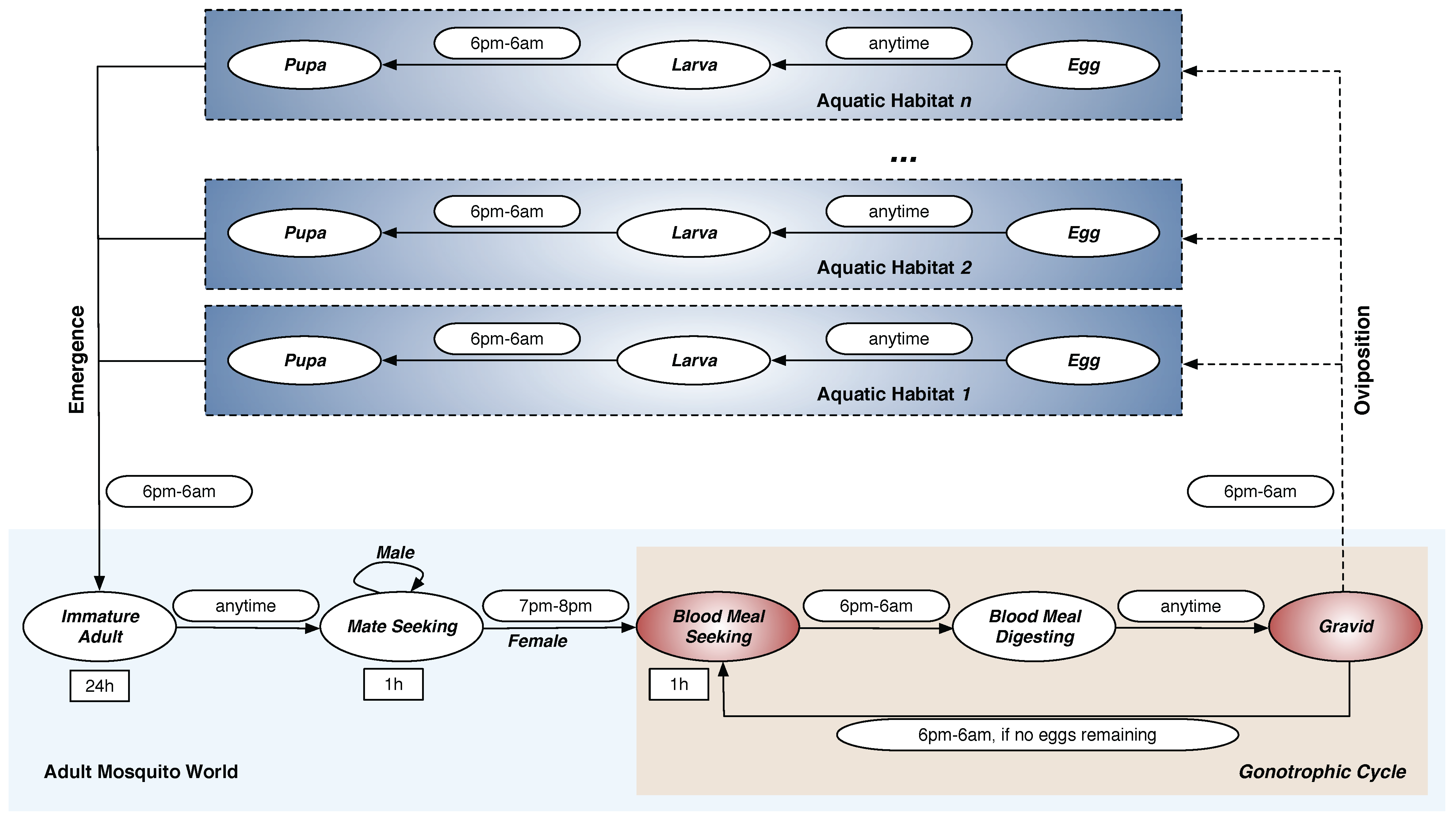
The complete An. gambiae mosquito life cycle consists of aquatic and adult phases, as shown in Figure 1. The aquatic phase (also known as the immature phase) consists of three aquatic stages: Egg (E), Larva (L), and Pupa (P). The adult phase consists of five adult stages: Immature Adult (IA), Mate Seeking (MS), Blood Meal Seeking (BMS), Blood Meal Digesting (BMD), and Gravid (G) (the term gravid denotes the egg-laying stage). The development and mortality rates in all eight stages of the life cycle are described in terms of the aquatic and adult mosquito populations.

The core model addresses several important features of the An. gambiae life cycle, including the development and mortality rates in different stages, the aquatic habitats, oviposition, etc. Another important feature, vector senescence, is adopted to account for the age-dependent aspects of the mosquito biology, and implemented using density- and age-dependent larval and adult mortality rates. Further details about the core model can be found in [16].

The Anopheles mosquitoes need to access human blood meals (in houses) and aquatic habitats (various water bodies) to complete their life cycle. Thus, the houses and aquatic habitats can be termed as important ecological resources for the mosquitoes. These resources have a direct impact on the spatial heterogeneity of the landscapes being modeled, and their availability has long been recognized as a crucial determinant for malaria transmission [20].

Figure 1. Life Cycle of Mosquito Agents. The An. gambiae mosquito life cycle consists of aquatic and adult phases. The aquatic phase consists of three aquatic stages: Egg (E), Larva (L), and Pupa (P). The adult phase consists of five adult stages: Immature Adult (IA), Mate Seeking (MS), Blood Meal Seeking (BMS), Blood Meal Digesting (BMD), and Gravid (G). Each oval represents a stage in the model. Stages in which agents move through the landscape are marked in red. The rectangles represent durations for the fixed-duration stages. The symbol h denotes hour. Permissible time transition windows (from one stage to another) are shown next to the corresponding stage transition arrows as rounded rectangles. Note that adult males, once reaching the Mate Seeking stage, remain forever in that stage until they die; adult females cycle through obtaining blood meals (in Blood Meal Seeking stage), developing eggs (in Blood Meal Digesting stage), and ovipositing the eggs (in Gravid stage) until they die. By Arifin et al. [16], used under a Creative Commons Attribution 4.0 International License.

Figure 1. Life Cycle of Mosquito Agents. The An. gambiae mosquito life cycle consists of aquatic and adult phases. The aquatic phase consists of three aquatic stages: Egg (E), Larva (L), and Pupa (P). The adult phase consists of five adult stages: Immature Adult (IA), Mate Seeking (MS), Blood Meal Seeking (BMS), Blood Meal Digesting (BMD), and Gravid (G). Each oval represents a stage in the model. Stages in which agents move through the landscape are marked in red. The rectangles represent durations for the fixed-duration stages. The symbol h denotes hour. Permissible time transition windows (from one stage to another) are shown next to the corresponding stage transition arrows as rounded rectangles. Note that adult males, once reaching the Mate Seeking stage, remain forever in that stage until they die; adult females cycle through obtaining blood meals (in Blood Meal Seeking stage), developing eggs (in Blood Meal Digesting stage), and ovipositing the eggs (in Gravid stage) until they die. By Arifin et al. [16], used under a Creative Commons Attribution 4.0 International License.

2.2. Aquatic Habitats and Oviposition

The core model assumes simplistic, homogeneous aquatic habitats for all mosquitoes. All habitats are uniform in size and capacity (this assumption is relaxed for this study by including five different types of habitats with varying habitat capacities, as described in Table 2), and the water temperature of a habitat is assumed to be the same as the air temperature. To account for the combined seasonality factor, each aquatic habitat is set with a carrying capacity that can be below or above a baseline capacity, representing low or high precipitation/rainfall, respectively. The carrying capacity essentially represents the density-dependent oviposition mechanism by regulating an age-adjusted biomass that the habitat can sustain.

Table 2. Feature types and counts for the ABM. A total of 975 aquatic habitats and 941 houses are used. The last column represents the assigned capacity per feature.

Type	Count	Assigned Capacity
Pool	4	2000
Puddle	13	1000
Pit latrine	395	500
Borehole	4	300
Wetland	559	10
House	941	5

Table 2. Feature types and counts for the ABM. A total of 975 aquatic habitats and 941 houses are used. The last column represents the assigned capacity per feature.

Type	Count	Assigned Capacity
Pool	4	2000
Puddle	13	1000
Pit latrine	395	500
Borehole	4	300
Wetland	559	10
House	941	5

Oviposition is the process by which gravid female mosquitoes lay new eggs. The oviposition behavior of An. gambiae mosquitoes can be affected by a variety of factors, as demonstrated by several studies [21,22,23,24,25,26,27,28]. In the core model, all larvae are categorized into different age groups, or cohorts, according to the common age of the cohort. The model keeps track of the age-adjusted biomass in each aquatic habitat, which is defined as the sum of the eggs, the pupae, and the one-day old equivalent larval population in the habitat (for details, see [16]).

2.3. The Spatial Agent-Based Model (ABM)

The spatial ABM, described in detail in [14,15], simulates the life cycle of the mosquito vector An. gambiae by tracking attributes relevant to the vector population dynamics for each individual mosquito. It is developed in the Java [29] object-oriented programming (OOP) language using the Eclipse Software Development Kit (SDK, Version: 3.5.2, freely available from [30]). In this section, we present a brief overview.

The three major components of the spatial ABM are the mosquito agents, their environment, and rules. An. gambiae mosquitoes are modeled as autonomous agents with explicit spatial locations (however, once within a cell, a mosquito agent’s spatial location does not vary until it moves to another cell). An agent’s life in the ABM evolves in artificial, well-defined environments modeled as landscape environments. A landscape environment can be thought of as a medium on which the agents operate and with which they interact. Agents have internal attributes (states) to store relevant attributes and data represented by discrete variables. The major attributes of a mosquito agent include its age, life cycle stage, environment, spatial location, movement counter, id (identifier), sex (gender), available eggs counter, egg batch identifier, etc. Some attributes (e.g., id, sex) may remain fixed throughout the agent’s lifespan in the ABM, while others (e.g., age, life cycle stage, spatial location) may change through interaction with the environment and/or other agents.

In the ABM, An. gambiae mosquitoes are the only dynamic agents (humans are included as static agents, i.e., human agents do not move in space). A new mosquito agent begins its life cycle in the aquatic phase as an egg, and then proceed through larva and pupa stages. When the aquatic phase completes, the agent emerges as an adult mosquito into the adult phase, and advances through the five adult stages (see Figure 1). To account for the limited flight ability and perceptual ranges of Anopheles mosquitoes, the cell resolution in the selected landscape is chosen as 50 m × 50 m, yielding a total area of ≈25 km${}^2$ (for this study). Note that at every time step of the BMS and G stages, the agent needs to search the cell-based landscape by moving from one cell to another until the desired resource is found (the search event is guided by several flight heuristics, as described in Section 2.5). A male adult mosquito, after reaching the MS stage, stays in this stage for the rest of its life. The stage transitions (from one stage to another), development rates, and mortality rates are governed by rules as described by the core model. The number of eggs that a gravid mosquito agent can lay is governed by the density-dependent oviposition rules (see [16] for details). New agents, in the form of eggs, possess the same spatial locations as that of the aquatic habitat in which they are oviposited.

The GIS-processed data layers are synthesized in the spatial ABM with a landscape-based approach, where each landscape comprises discrete and finite-sized cells (grids). A landscape is used to represent the coordinate space necessary for the spatial locations of the environments and the adult mosquito agents. Resources, in the forms of aquatic habitats and houses, are contained within a landscape. Each cell, with its spatial attributes, may represent a specific habitat environment (human or aquatic), or be part of the (adult) mosquito environment. Landscapes are topologically modeled as 2D torus spaces with a non-absorbing (periodic) boundary (with a non-absorbing (periodic) boundary, when mosquitoes hit an edge of a landscape, they re-enter it from the edge directly opposite of the exiting edge, and thus are not killed due to hitting the edge).

2.4. Event Action List (EAL) Diagram

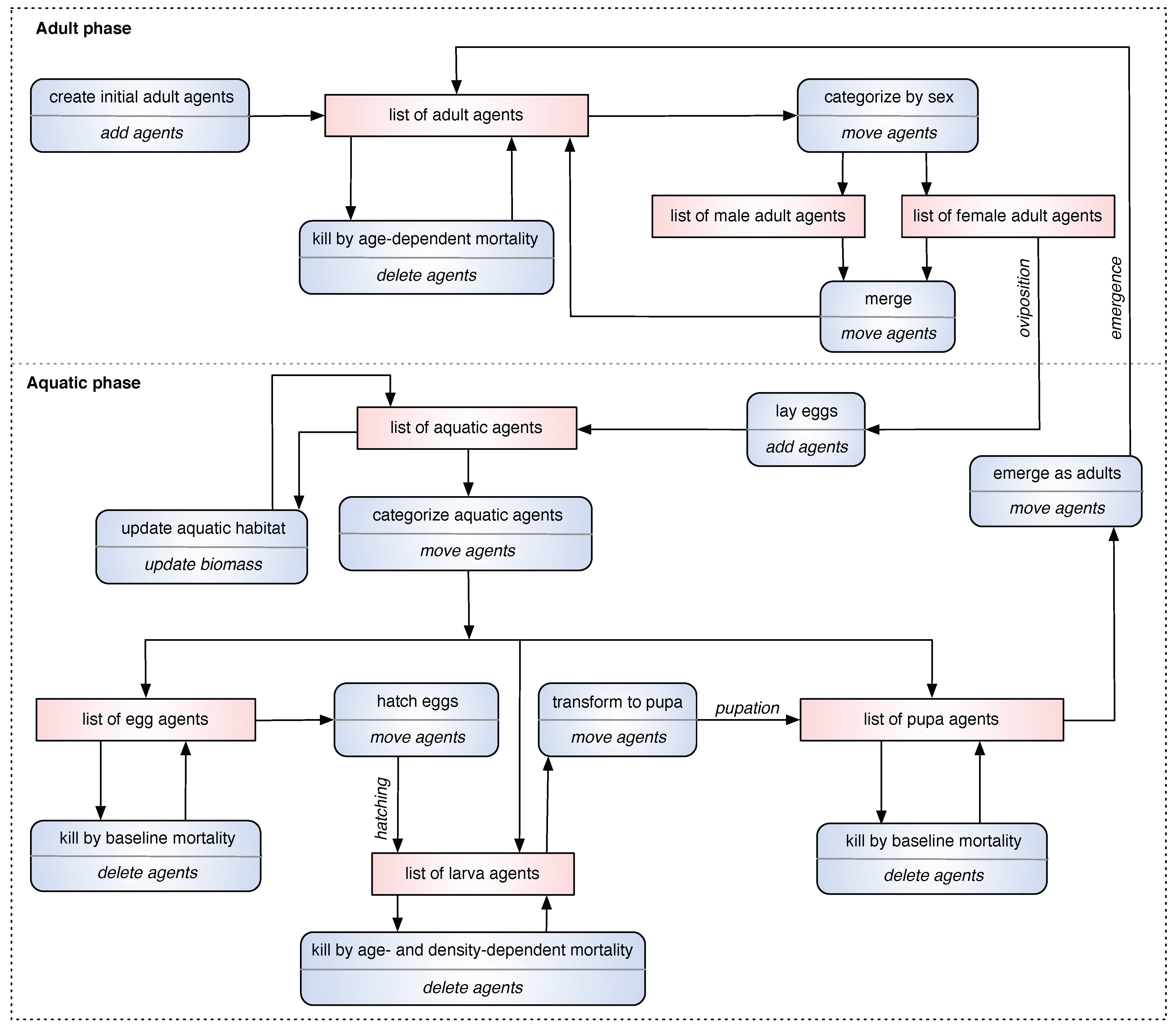
In order to capture the major daily events of a simulation for the ABM in a standard, canonical manner, a new type of descriptive diagram, called the Event Action List (EAL) diagram, is proposed and presented. It depicts the simulation events (occurring on a daily basis), the corresponding actions triggered by those events, and the list(s) of agents (data structures) affected by them. In an EAL diagram, each event represents a biological phenomenon, and the corresponding action represents the programmatic task(s) performed by the simulation. Optionally, some list(s) of agents may be modified as a direct result of the performed action. Thus, an EAL diagram summarizes the daily events of the simulation model by listing all major events, actions, and lists. For example, when the simulation is started, it needs to create initial adult mosquito agents. The biological phenomenon “create initial adults”, termed as an event, is realized by the (simulation) action “add agents”; this event-action pair affects the list of adult agents in the simulation. An EAL diagram for the ABM is shown in Figure 2.

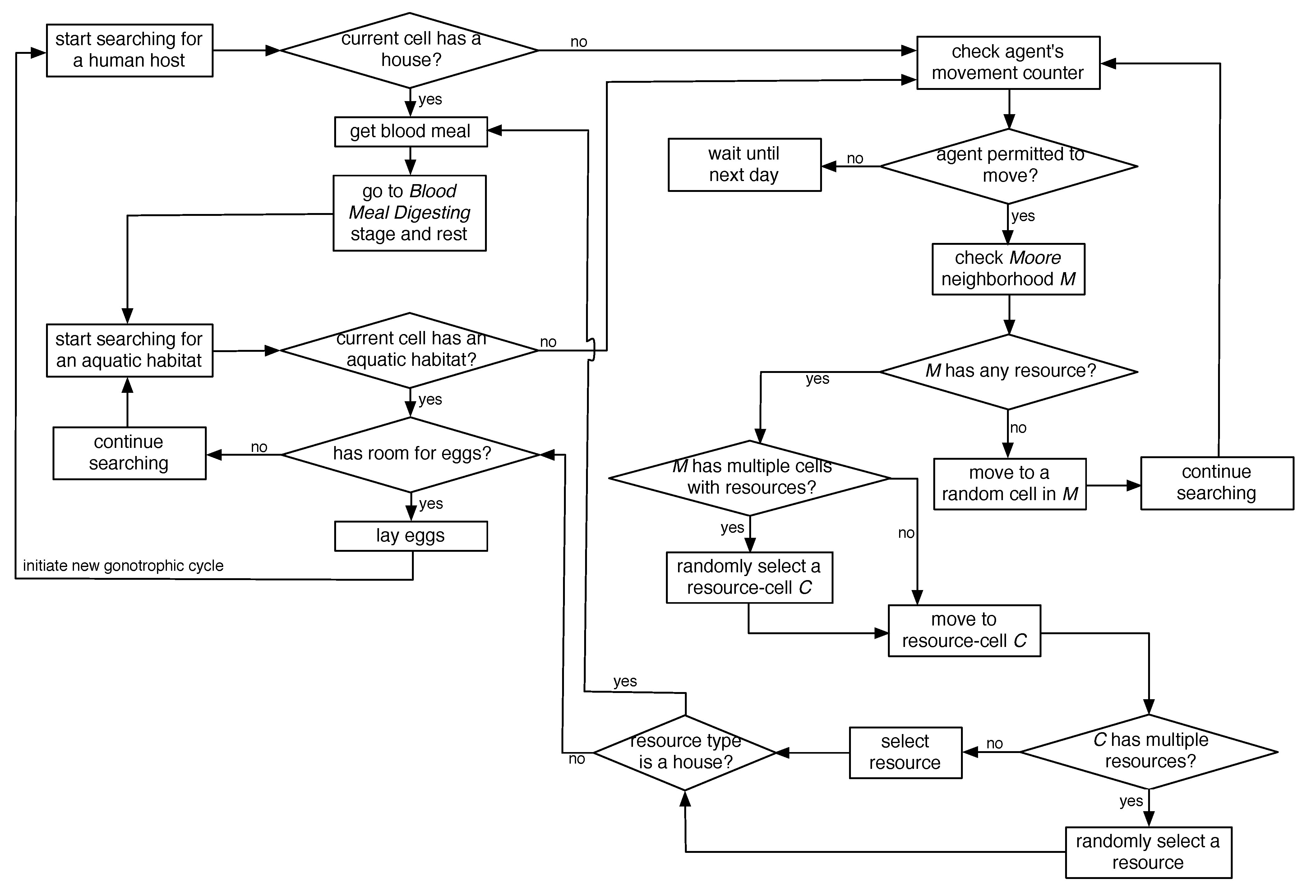
2.5. Flight Heuristics for Mosquito Agents

In the spatial ABM, movement of adult female mosquito agents in a landscape is restricted: they move only when in BMS and G stages (marked in red in Figure 1) in order to seek for resources. Since each landscape comprises discrete and finite-sized (50 m × 50 m) cells, the landscape-based modeling approach appeared to be especially suitable to capture the details of the resource-seeking process. In summary, the resource-seeking process is modeled with random non-directional flights with limited flight ability and perceptual ranges until the agents can perceive resources at close proximity, at which point, the flight becomes directional.

Figure 2. An Event Action List (EAL) diagram for the ABM. Each squashed rectangle represents an event-action pair, in which the event is denoted at the upper-half, and the action is denoted at the lower-half. Each rectangle represents the list(s) (data structures) of agents affected by the event-action pair.

Figure 2. An Event Action List (EAL) diagram for the ABM. Each squashed rectangle represents an event-action pair, in which the event is denoted at the upper-half, and the action is denoted at the lower-half. Each rectangle represents the list(s) (data structures) of agents affected by the event-action pair.

A mosquito agent’s neighborhood is modeled as an eight-directional Moore neighborhood. The maximum distance that an agent may travel in a day is controlled by a movement counter, which is reset to 5 at the beginning of each day for a moving agent (thus, the counter controls the maximum daily range of movement, which translates to $250\sqrt[2]{2}$ m). The flight heuristics, depicted in the form of flow-charts in Figure 3, are described below.

The host-seeking event starts when a female adult mosquito agent enters the BMS stage and searches for a human blood meal in a house. If the current cell contains a house, it immediately gets a blood meal, and enters the BMD stage to digest the meal, rest, generate new eggs, and eventually enter the G stage to search for an aquatic habitat (if the current cell contains multiple houses, one is chosen at random). If the current cell does not contain any house, a new search event starts as follows. First, the agent’s movement counter is checked. If the agent is permitted to move, its Moore neighborhood M is checked. If M contains multiple cells that have houses, a random cell C (from these cells) is selected, and the agent moves to cell C. If cell C contains multiple houses, a random house is selected, the agent gets a blood meal, and continues as before. However, if the current cell and its Moore neighborhood do not contain any house, the agent starts a random flight and moves randomly into one of the adjacent eight cells (following a previous study [31], the probability of a random move into a diagonally-adjacent cell is set as half that of moving into a horizontally- or vertically-adjacent cell).

Figure 3. Flight heuristics for mosquito agents.

Figure 3. Flight heuristics for mosquito agents.

In an oviposition event, an agent searches for an aquatic habitat. If the current cell contains an aquatic habitat, it’s current capacity is checked to see if it has any remaining capacity for new eggs, in which case, the agent lay the eggs (again, if the current cell contains multiple aquatic habitats, one is chosen at random). Once all of the eggs are laid, it goes to the BMS stage, thus initiating a new gonotrophic cycle. If the current cell does not contain any aquatic habitat, the search continues in the same fashion as described above.

As evident from the above, in case of a directional flight, if multiple resources (houses or aquatic habitats) are found within a single cell, a random resource is selected. Note that this strategy can be easily extended/modified for future work to select a resource based on some preference criterion, e.g., to select the house which has the fewest number of mosquitoes visited or to select the aquatic habitat which has the largest remaining capacity.

As evident from the above, in case of a directional flight, if multiple resources (houses or aquatic habitats) are found within a single cell, a random resource is selected. Note that this strategy can be easily extended/modified for future work to select a resource based on some preference criterion, e.g., to select the house which has the fewest number of mosquitoes visited or to select the aquatic habitat which has the largest remaining capacity.

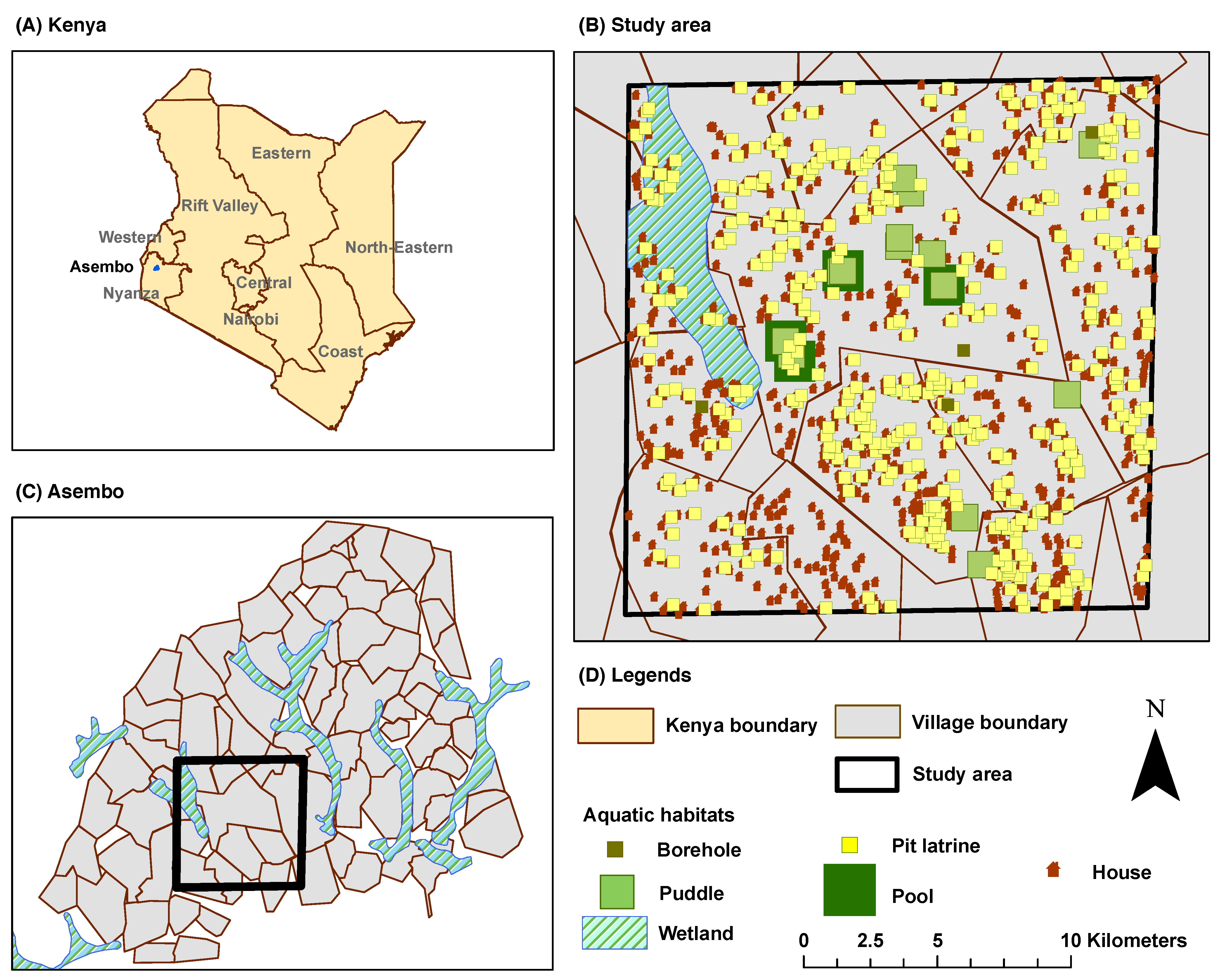
2.6. The Study Area

The study area is located within a subsection of the Siaya and Bondo Districts (Rarieda Division, Nyanza Province) in western Kenya. It comprises a village which is selected from a set of 15 villages with an area of approximately 70 km${}^2$. The greater area is locally known as Asembo, which covers an area of 200 km${}^2$ with a population of approximately $60,000$ persons [32]. It lies on Lake Victoria and experiences intense, perennial (year-around) malaria transmission [33]. The primary reason for selecting Asembo is the availability of relevant data from the Asembo Bay Cohort Project [34] and the Asembo ITN project [32]. In a series of 23 articles, these studies reported important public health findings from a successful trial of ITNs in western Kenya [35]. The study area is shown in Figure 4: Figure 4A shows the boundary and administrative units for Kenya, Figure 4B shows the selected data layers within the village cluster, and Figure 4C shows the selected village cluster in Asembo, Kenya.

The ABM, without explicit parallelization or multiple runs, can handle a landscape with finite maximum dimensions. Hence, a subset of villages with $95\times 96$ cell dimensions is selected for all simulation runs in this study, as outlined by the polygons in Figure 4B,C.

2.7. GIS Processing of Data Layers

ArcGIS Desktop 10 [36] is used to produce, process, and analyze the relevant data layers. Different types of water features and villages (including houses) are identified, extracted and projected to the Arc 1950 UTM Zone 36S projection system for all over Kenya. The selected water features include rivers, lakes, wetlands, wells/springs, falls/rapids, lagoons, etc. Each water feature type is assigned a unique ID.

The selected features are scaled down to a village cluster around Asembo. Water features for different types of aquatic sites are included. Since the spatial ABM deals with spatial features at the habitat levels, the study area is further scaled down to village and household levels, and then to subsets of villages levels. Some of the water features are ranked by precedence by sub-grouping the water source data layers based on their attributes. Similar types of water features in the same data layer are combined.

The selected data layers are then converted to the raster format, with a cell resolution of 50 m × 50 m. All point shapefiles for aquatic habitats and houses are converted using the Point to Raster tool. Since pit latrines are usually found inside the household boundaries, the shapefile for pit latrines is created from the shapefile for houses. It is possible to have more than one feature type within a single cell. In these cases, to calculate the number of features (of each type) in each cell, the summation of value fields of the corresponding data features is used. Finally, the raster files are converted to the ASCII format, and are ready to be used as input to the spatial ABM.

Figure 4. The Study Area. (A) Kenya Boundary and Administrative Units (Provinces); (B) Study Area with Selected Data Layers; the outlined polygon represents a subset of villages selected for the simulation runs in this study; (C) Village Cluster in Asembo; (D) Legends.

Figure 4. The Study Area. (A) Kenya Boundary and Administrative Units (Provinces); (B) Study Area with Selected Data Layers; the outlined polygon represents a subset of villages selected for the simulation runs in this study; (C) Village Cluster in Asembo; (D) Legends.

2.8. Feature Counts

A total of 975 aquatic habitats, categorized into five different types, are identified in the selected area as follows: (1) pools (large); (2) puddles (small); (3) pit latrines; (4) boreholes; and (5) wetland. Boreholes, also known as borrow pits, have significant potential as breeding sites in the area. They represent man-made holes or pits in the ground when local people use clay or soil for building houses, making pots, etc., thereby leaving depressions in the ground that easily get filled with rain water. Pit latrines are very common to the households in the area. The wetland represents a stretch of marsh lying to the northwest corner of the area which is dominated by herbaceous plant species.

As mentioned before, each aquatic habitat is set with a predefined carrying capacity ($CC$), which regulates the aquatic mosquito population that the habitat can sustain, and reflects the habitat heterogeneity (e.g., in terms of productivity) to some degree (see [15] for details). A total of 941 houses, each having a mean of five occupants, are also identified. These feature counts and their assigned values are summarized in Table 2. Note that for wetland, which covers multiple cells in the northwest corner of the study area, the same $CC$ value is assigned to each cell.

2.9. Vector Control Interventions

The last decade (2000–2010) of worldwide malaria control efforts has seen an unprecedented increase in the coverage of vector (mosquito) control interventions for malaria, with ITNs/LLINs, IRS, and LSM as the front-line vector control tools [37]. These interventions are often applied in isolation and in combination, and their impacts have been investigated by numerous early and recent studies [38,39,40,41,42,43,44,45]. In addition to these time-tested, established tools, new and novel intervention tactics and strategies such as new drugs, vaccines, insecticides, improved surveillance methods, etc., are also being investigated [46]. Some of the promising approaches include genetically engineered mosquitoes through sterile insect technique (SIT) or release of insects containing a dominant lethal [47,48], fungal biopesticides that increase the rate of adult mosquito mortality [49], the development of genetically modified mosquitoes (GMMs) or transgenic mosquitoes manipulated for resistance to malaria parasites [50], transmission blocking vaccines (TBVs) which are intended to induce immunity against the malaria parasites [51], etc.

As mentioned before, the combined impacts of two vector control interventions (LSM and ITNs) are evaluated for this study. Both interventions have been extensively used as intervention tactics to reduce and control malaria in sub-Saharan Africa, as reported by numerous early and recent studies [37,39,41,53]. LSM (also known as source reduction) is one of the oldest tools in the fight against malaria. It refers to the management of aquatic habitats in order to restrict the completion of immature stages of mosquito development. ITNs, particularly LLINs, are considered among the most effective vector control strategies currently in use [39,52]. ITNs offer direct personal protection to users as well as indirect community protection to non-users (through insecticidal and/or repellent effects). For this study, LSM refers to the permanent elimination of targeted aquatic habitats. For ITNs, the household-level complete coverage scheme is used, which ensures that if a house is covered, all persons in the house are protected by bed nets; the two other relevant variables, killing effectiveness and repellence, are both fixed at 50%. Killing effectiveness refers to an increased mortality (increased probability of death of a mosquito), toxicity, or killing efficiency due to the insecticidal killing effects of the ITNs; the insecticide kills the mosquitoes that come into contact with the ITNs. Repellence refers to the insecticidal excito-repellent properties of the ITNs which repel the blood meal seeking mosquitoes; it adds a chemical barrier to the physical one, further reducing human-mosquito contact and increasing the protective efficacy of the ITNs (see [15,16] for details).

Four different scenarios are constructed by using two coverage (C) levels of $low$ $(20\%)$ and $high$ $(80\%)$. For a specific coverage, aquatic habitats and houses which will be covered by the corresponding intervention are selected by using random sampling. The actual numbers of objects covered approximate the desired coverage levels. A baseline scenario (with no intervention) is also added for comparison. The scenarios are summarized in Table 3.

Table 3. Scenarios obtained by applying the two vector control interventions LSM and ITNs. A total of 975 aquatic habitats and 941 houses are used to calculate the desired coverage (C) levels of $low(20\%)$ and $high(80\%)$. The first column denotes the scenario (interventions applied). The actual coverage (C) levels are given in the last two columns for aquatic habitats and houses covered in the landscape, respectively.

Scenario	Coverage (C) %
	% Aquatic Habitats Covered	% Houses Covered
$Baseline$	0	0
$LS{M}_{Low}-ITN{s}_{Low}$	$208/975=0.21$	$204/941=0.22$
$LS{M}_{Low}-ITN{s}_{High}$	$215/975=0.22$	$751/941=0.8$
$LS{M}_{High}-ITN{s}_{Low}$	$774/975=0.79$	$195/941=0.21$
$LS{M}_{High}-ITN{s}_{High}$	$781/975=0.8$	$736/941=0.78$

Table 3. Scenarios obtained by applying the two vector control interventions LSM and ITNs. A total of 975 aquatic habitats and 941 houses are used to calculate the desired coverage (C) levels of $low(20\%)$ and $high(80\%)$. The first column denotes the scenario (interventions applied). The actual coverage (C) levels are given in the last two columns for aquatic habitats and houses covered in the landscape, respectively.

Scenario	Coverage (C) %
	% Aquatic Habitats Covered	% Houses Covered
$Baseline$	0	0
$LS{M}_{Low}-ITN{s}_{Low}$	$208/975=0.21$	$204/941=0.22$
$LS{M}_{Low}-ITN{s}_{High}$	$215/975=0.22$	$751/941=0.8$
$LS{M}_{High}-ITN{s}_{Low}$	$774/975=0.79$	$195/941=0.21$
$LS{M}_{High}-ITN{s}_{High}$	$781/975=0.8$	$736/941=0.78$

2.10. Simulations

For each of the five scenarios ($Baseline$, $LS{M}_{Low}-ITN{s}_{Low}$, $LS{M}_{Low}-ITN{s}_{High}$, $LS{M}_{High}-ITN{s}_{Low}$, and $LS{M}_{High}-ITN{s}_{High}$), 50 replicated simulation runs are performed and the average results are reported (in order to rule out any stochasticity effects). Each simulation runs for 730 days (2 years) (in this paper, all time units related to the simulation runs refer to simulated time as opposed to physical time or wall clock time; thus, a 2 years run indicates a virtual simulation run within the computer which represents an imitation of operations in the real-world for the same time duration), and reaches a steady state (equilibrium) at around day 50. Interventions are applied on day 100 and continued up to the end of the simulation.

Initially, all simulations start with 1000 female adult mosquito agents (no male agents). Each female agent is assigned to a randomly-selected aquatic habitat. The maximum daily range of movement for mosquito agents is set to 5 cells per day, which translates to $250\sqrt[2]{2}$ m. Biological aging (senescence) of the mosquitoes is assumed. The ABM implements age-specific mortality rates for the adult mosquitoes and the larvae (i.e., the probability of death for mosquito agents increases with their age).

2.11. Output Indices

Mosquito abundance is the primary output index of the ABM. However, the spatial model also allows us to explore some spatial indices by overlaying these on the entire landscape. These indices capture the spatial heterogeneity of various objects (aquatic habitats and houses) in the landscape. Some of these indices are generated as cumulative aggregates at the end of each simulation run, and represent measures on a per object basis. The output indices are listed below:

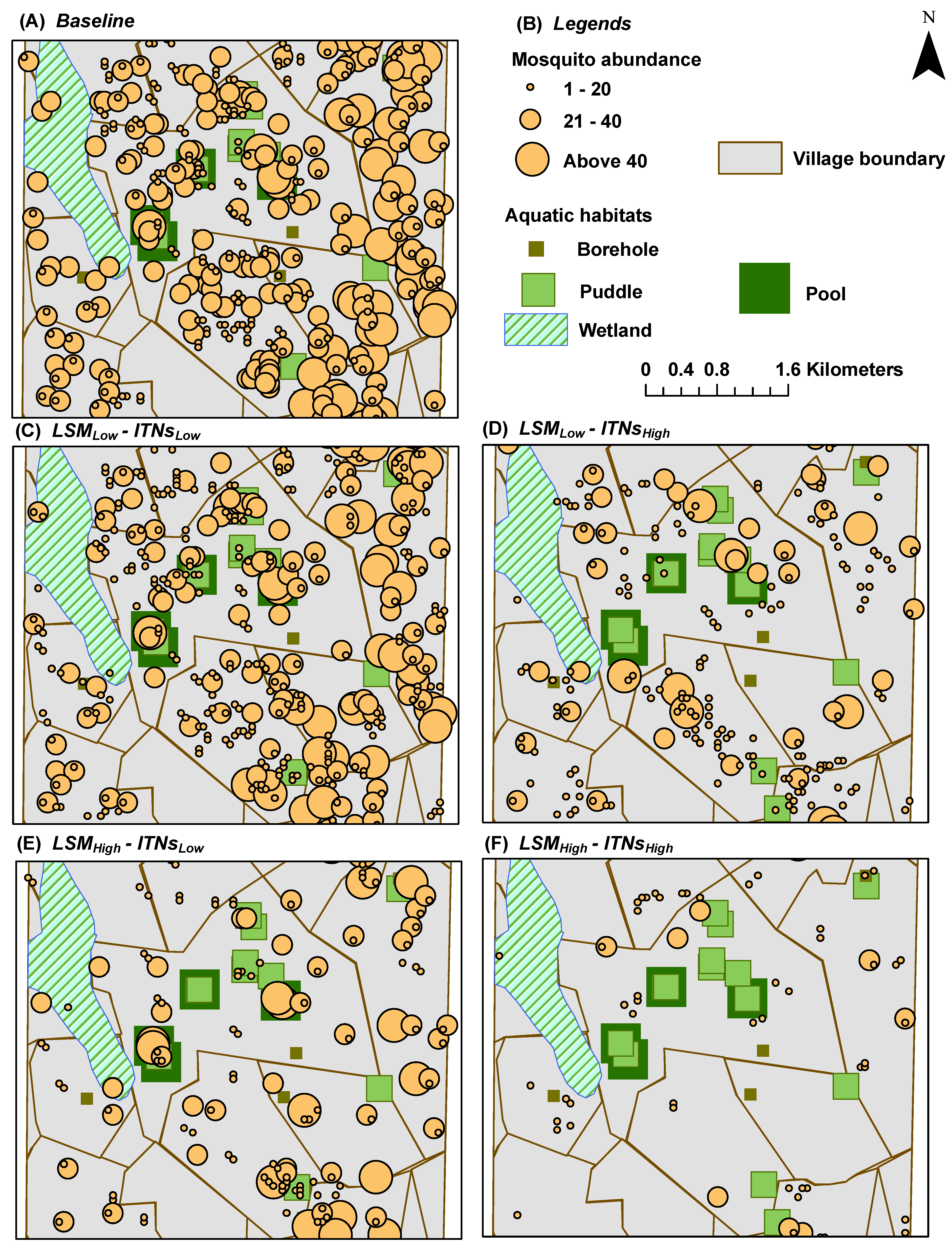
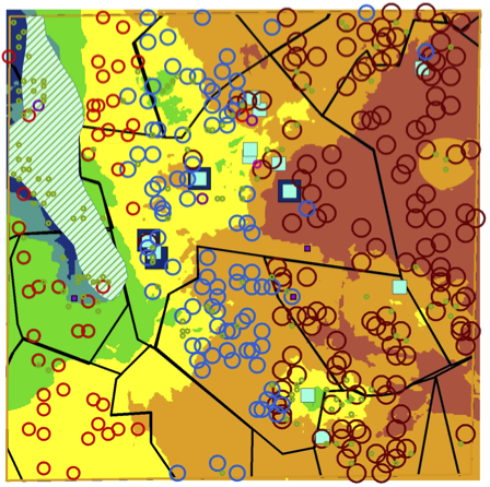
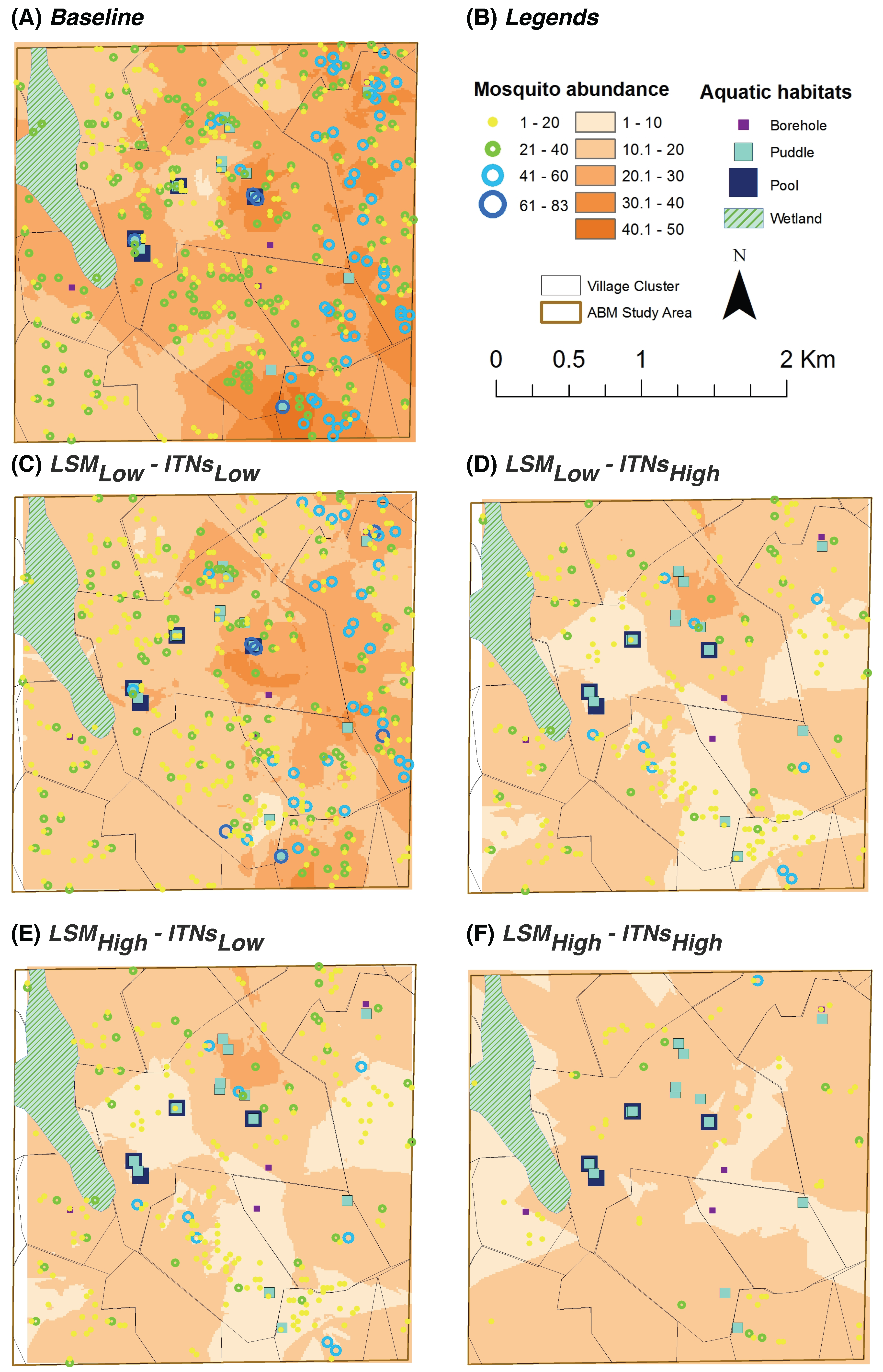
• Mosquito Abundance: represents a spatial snapshot of the female adult mosquito population distribution at the end of simulations (see Figure 5 and Figure 6)
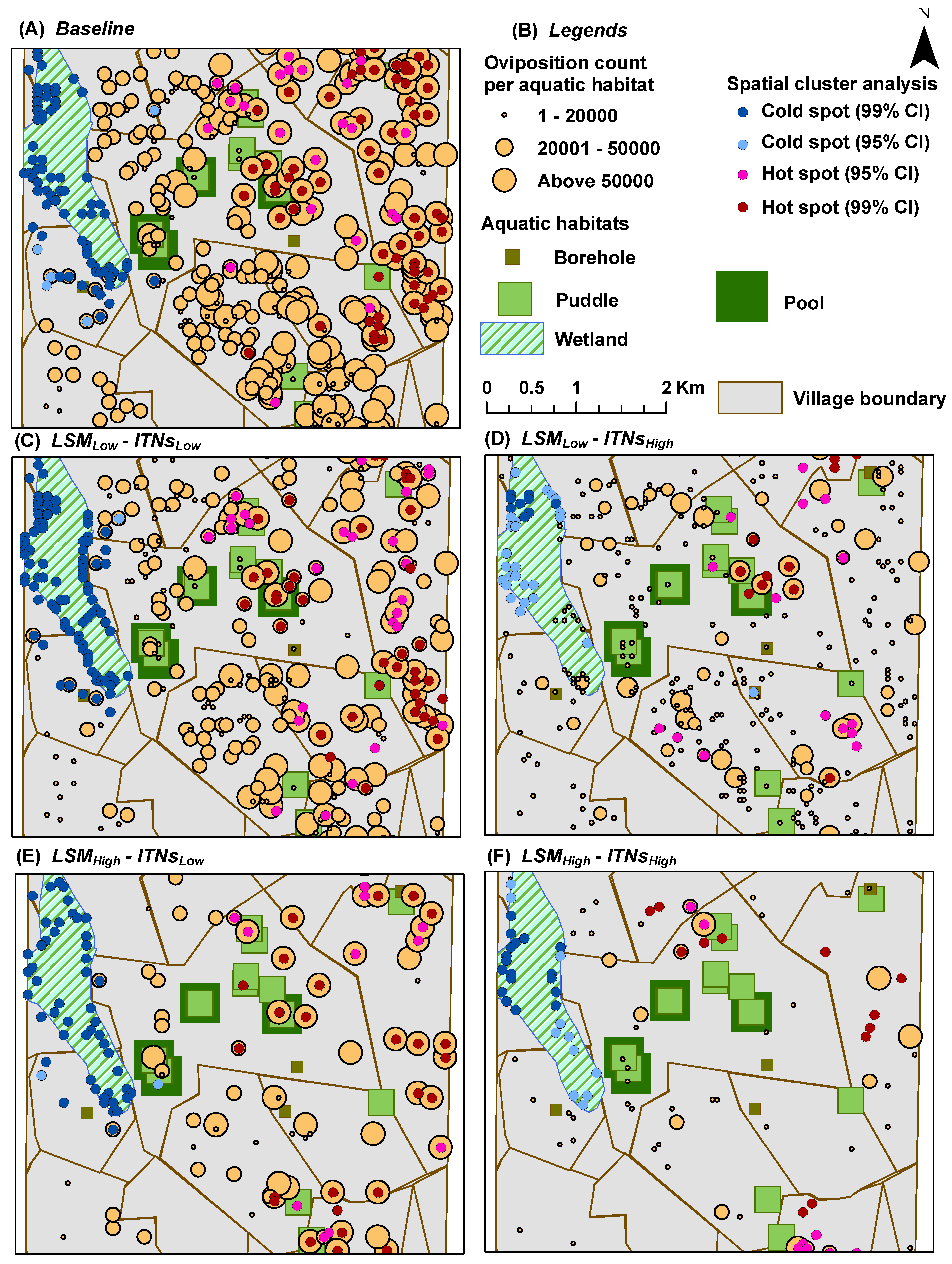
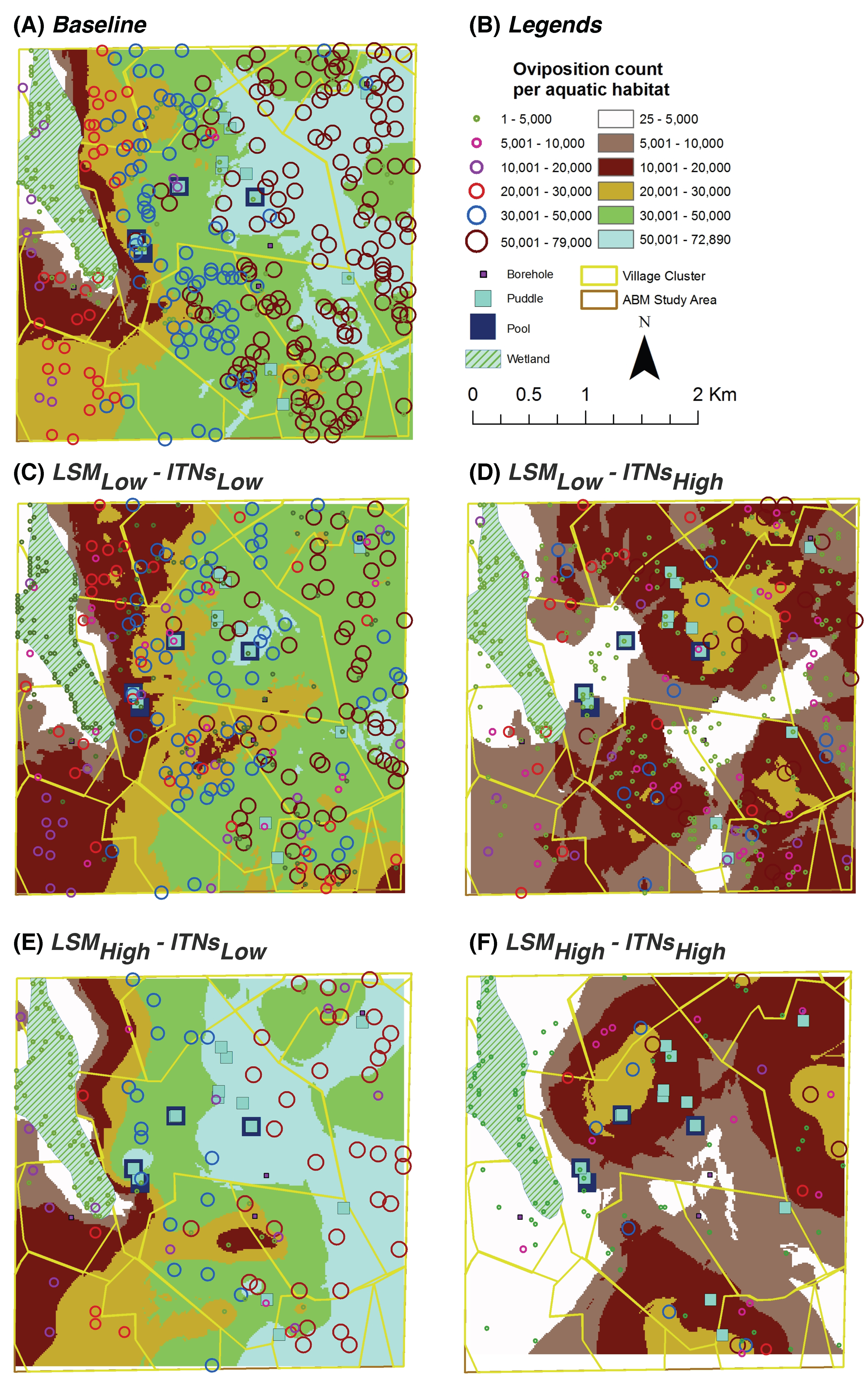
• Oviposition Count per Aquatic Habitat: for each aquatic habitat x, it represents the cumulative number of female adult mosquitoes which have oviposited (laid eggs) in x; depicted spatially at the end of simulations by overlaying on top of the aquatic habitats (see Figure 7 and Figure 8)
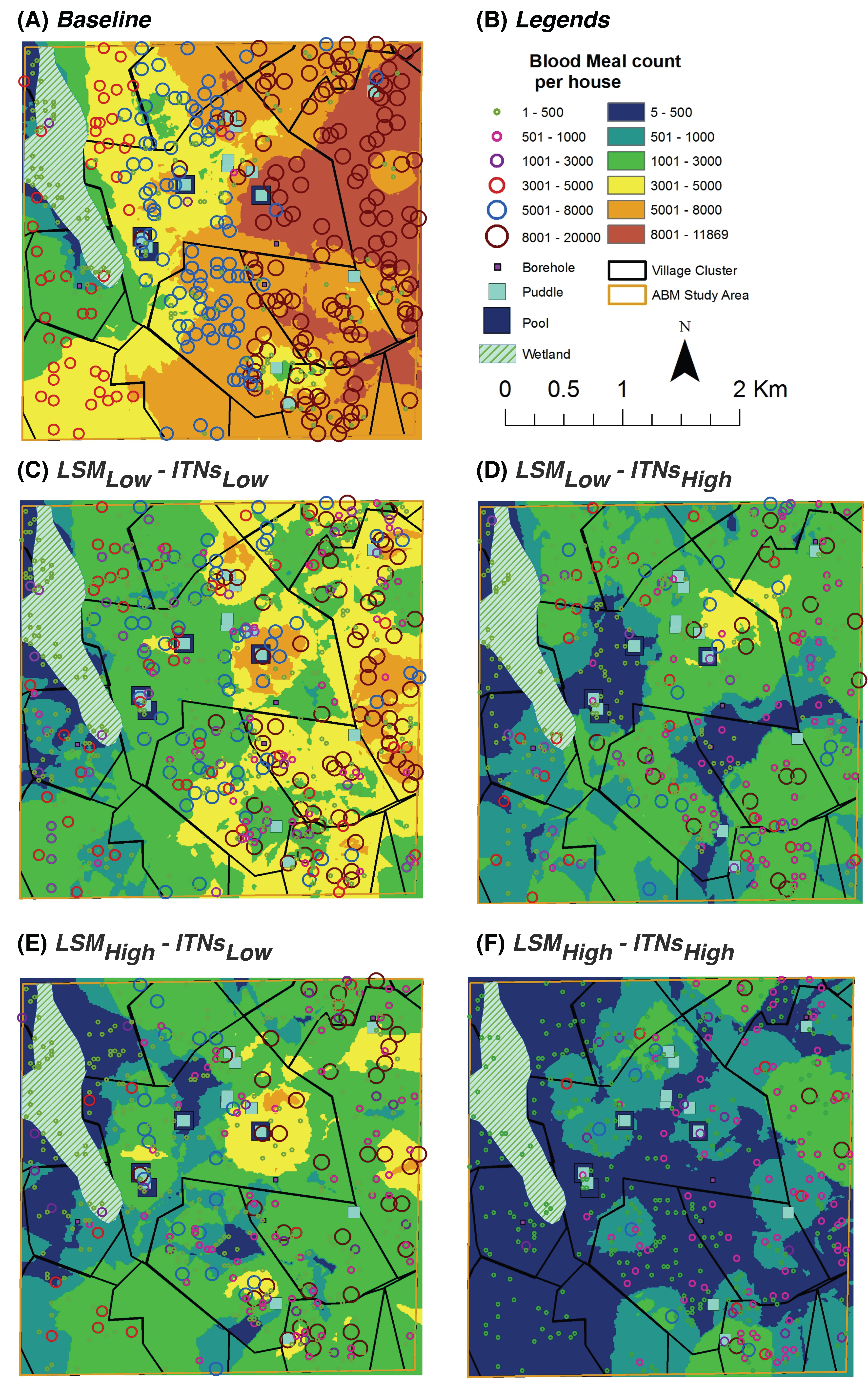
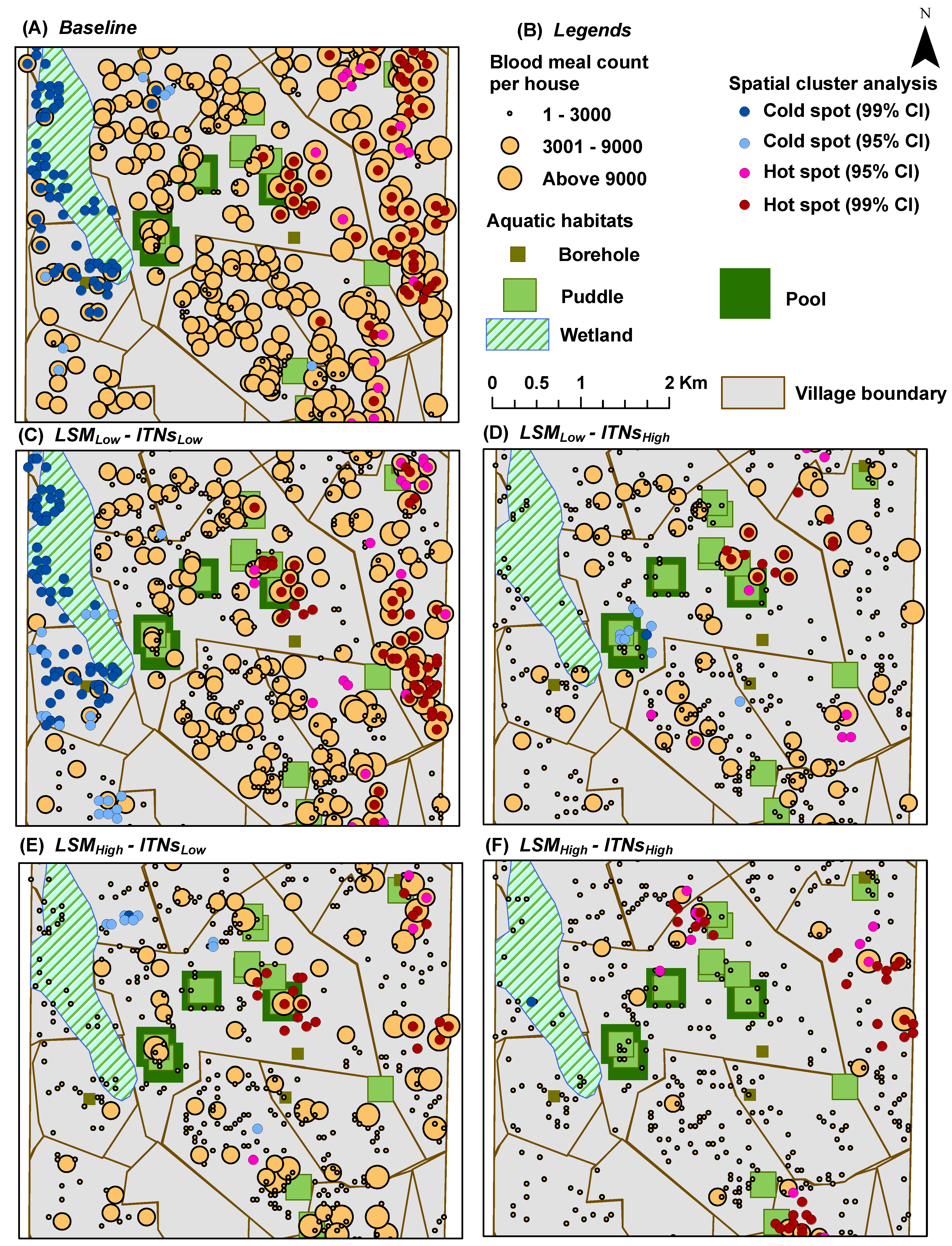
• Blood Meal Count per House: for each house y, it represents the cumulative number of blood meals successfully obtained by female adult mosquitoes in y; depicted spatially at the end of simulations by overlaying on top of the houses (see Figure 9 and Figure 10)

Note that for all output indices, the average measures of 50 replicated simulation runs are reported (in order to rule out any stochasticity effects). The spatial indices are sampled across all daily time steps throughout the entire simulations. The output maps are produced by overlaying the averaged indices on top of the relevant data layers.

All output indices are mapped using the graduated symbology. The graduated symbol renderer is one of the common renderer types used to represent quantitative information. Using a graduated symbols renderer, the quantitative values for the output indices are separately grouped into ordered classes, so that higher values cover larger areas on the map. Within a class, all features are drawn with the same symbol. Each class is assigned a graduated symbol from the smallest to the largest.

2.12. Hot Spot Analysis

Using spatial statistics tools, hot spot analysis (spatial cluster analysis) is performed for all scenarios for the last two indices (oviposition count per aquatic habitat and blood meal count per house) in order to determine whether a specific value is statistically significant or not [53]. In hot spot analysis, if a higher value is surrounded by similar magnitude of other higher values, it is considered a hot spot (with $95\%$ or $99\%$ confidence intervals). The cold spots are determined using the same principle. The values (or cluster of values) between the statistically significant hot spots and cold spots are considered as random samples of a distribution. The hot spot analysis tool calculates the Getis-Ord Gi* statistic (z-scores and p-values) for each feature in a dataset [36]. Z-scores are measures of standard deviations, and define the confidence intervals (in this case, $95\%$–$99\%$). A p-value represents the probability that the observed spatial pattern was created by some random process.

The null hypothesis for pattern analysis essentially states that the expected pattern is just one of the many possible versions of complete spatial randomness. If the z-score is within the $95\%$–$99\%$ confidence interval or beyond, the exhibited pattern is probably too unusual to be of random chance, and the p-value will be subsequently small to reflect this. In this case, it is possible to reject the null hypothesis and proceed to determine the cause of the statistically significant spatial pattern. On the other hand, if the z-score lies below the $95\%$ confidence interval, the p-value will be larger, the null hypothesis cannot be rejected, and the pattern exhibited is more likely to indicate a random pattern. Thus, a high z-score and small p-value for a feature indicates a significant hot spot. Conversely, a low negative z-score and small p-value indicates a significant cold spot.

2.13. Kriging Analysis

Kriging, also known as Gaussian process regression, is a popular method of interpolation (prediction) for spatial data. It is an interpolation technique in which the surrounding measured values are weighted to derive a predicted value for an unmeasured location. Weights for the measured values depend on the distance between the measured points, the prediction locations, and the overall spatial arrangement among the measured points [54]. Various kriging techniques provide a framework for predicting values of a variable of interest at unobserved locations given a set of spatially distributed data, incorporating spatial autocorrelation and computing uncertainty measures around model predictions [55,56].

In recent years, kriging has been extensively used in public heath and epidemiology modeling for variable mapping to interpolate estimates of occurrence of a variable or risk of disease [57,58,59]. For example, de Carvalho Alves and Pozza characterized the spatial variability of common bean anthracnose using kriging and nonlinear regression models [60]. Alexeeff et al. evaluated the accuracy of epidemiological health effect estimates in linear and logistic regression when using spatial air pollution predictions from kriging and land use regression models [61]. For malaria modeling, the Malaria Atlas Project (MAP) [62] developed several Bayesian geostatistical kriging models for spatial prediction of Plasmodium falciparum prevalence, estimated human populations at risk, vector distribution, etc., generating malaria maps of many endemic countries in sub-Saharan Africa [63,64,65].

The basic idea of kriging is to predict the value of a function at a given point by computing a weighted average of the known values of the function in the neighborhood of the point. To this end, kriging is closely related to the method of regression analysis. The data represent a set of observations of some variable(s) of interest, with some spatial correlation. Usually, the result of kriging is the expected value, referred to as the kriging mean and the kriging variance computed for every point within a region of interest. If kriging is done with a known mean, it is then called simple kriging. On the other hand, in ordinary kriging, estimating the mean and applying (simple) kriging are performed simultaneously.

Kriging uses semivariogram functions to describe the structure of spatial variability. A semivariogram is one of the significant functions to indicate spatial correlation in observations measured at sample locations, and plays a central role in the analysis of geostatistical data using kriging. The effect of different semivariograms on kriging has also been a focus of interest in different branches of the literature (e.g., [66]). In this paper, spatial analysis is conducted using ordinary kriging with circular semivariograms for all scenarios for all the output indices using ArcGIS 9.3 [19]. We note that similar analyses have also been conducted for other insects in the literature (e.g., for fig fly [67]).

3. Results

In this section, we describe the results by categorizing them according to the output indices. For the output indices and scenarios (see Table 3), simulation results are presented along with hot spot analysis and kriging results. For clarity, houses and pit latrines are not shown in the output maps. Each scenario (in the output maps) represents the average results of 50 replicated simulations.

3.1. Mosquito Abundance

The mosquito abundance maps are shown in Figure 5. These maps depict the mosquito abundances index, which represent a spatial snapshot of the female adult mosquito population distribution at the end of simulations. Figure 5A shows the abundance map for the baseline scenario (in which no intervention was applied). Figure 5B depicts the symbols used in the maps: it shows the village boundary, different types of aquatic habitats, and the graduated symbols for abundances. Note that for the aquatic habitats, the symbol sizes vary according to the assigned carrying capacities of the habitats (see Table 2). The symbol sizes for abundances also vary depending on the magnitudes. Figure 5C–F show the abundance maps for the four different scenarios with control interventions LSM and ITNs having two coverage levels: $LS{M}_{Low}-ITN{s}_{Low}$, $LS{M}_{Low}-ITN{s}_{High}$, $LS{M}_{High}-ITN{s}_{Low}$, and $LS{M}_{High}-ITN{s}_{High}$, respectively. The corresponding kriged maps for mosquito abundance are illustrated in Figure 6.

As shown in Figure 5, with increasing coverage levels of both interventions, the mosquito abundances are significantly reduced, as evident from the progressively lower number of “Above 40” symbols (which denote the highest abundances) in the series of figures. The changes are more clear and evident from the kriged maps (Figure 6).

It is interesting to note that ITNs are more effective in reducing abundances than LSM (compare Figure 5D,E as well as the kriged maps in Figure 6D,E): covering $80\%$ of the houses has more impact than removing a total of $80\%$ different types of the aquatic habitats. This is partially due to the fact that the household-level complete coverage scheme (used for ITNs, see Experimental Section) prohibits a blood meal-seeking female mosquito to obtain a blood meal from any person in any house which is covered by ITNs. As coverage of ITNs increases, more houses fall within the range of coverage, and the probability of finding an unprotected human in another house (during the blood meal-seeking stage) decreases. Thus, with increasing coverage of ITNs, abundances are reduced more effectively.

The $low(20\%)$ coverage levels for both interventions do not produce significant reduction in abundances, as evident from the baseline and $LS{M}_{Low}-ITN{s}_{Low}$ maps (compare Figure 5A,C). In general, higher abundances are observed near the pools (which have the highest carrying capacities) and in the north east and the south east portions of the map.

When either of the interventions has a $high(80\%)$ coverage level, abundances are significantly reduced, as evident from the $LS{M}_{Low}-ITN{s}_{High}$ and $LS{M}_{High}-ITN{s}_{Low}$ maps. For these two scenarios, the highest abundances observed are significantly lower than the baseline (compare Figure 5D,E with Figure 5A). However, for the $LS{M}_{Low}-ITN{s}_{High}$ scenario higher abundances do not always coincide with the spatial locations of aquatic habitats with higher carrying capacities, while for the other scenario this expected trend is observed for some cases.

Not surprisingly, when both interventions have $high(80\%)$ coverage levels, abundances are reduced to the lowest level, as evident from the $LS{M}_{High}-ITN{s}_{High}$ map shown in Figure 5F. For this scenario very few higher abundances are observed; these occur at greater distances from the spatial locations of aquatic habitats with higher carrying capacities, since most of them are eliminated by LSM.

Figure 5. Maps for all scenarios for the mosquito abundances index. Each scenario represents the average results of 50 replicated simulations. (A) Abundance map for baseline; (B) Legends: symbol sizes are proportional to the carrying capacities of the aquatic habitats (see Table 2); graduated symbol sizes are proportional to the magnitudes of abundances. For clarity, houses and pit latrines are not shown; (C) Abundance map for $LS{M}_{Low}-ITN{s}_{Low}$; (D) Abundance map for $LS{M}_{Low}-ITN{s}_{High}$; (E) Abundance map for $LS{M}_{High}-ITN{s}_{Low}$; (F) Abundance map for $LS{M}_{High}-ITN{s}_{High}$.

Figure 5. Maps for all scenarios for the mosquito abundances index. Each scenario represents the average results of 50 replicated simulations. (A) Abundance map for baseline; (B) Legends: symbol sizes are proportional to the carrying capacities of the aquatic habitats (see Table 2); graduated symbol sizes are proportional to the magnitudes of abundances. For clarity, houses and pit latrines are not shown; (C) Abundance map for $LS{M}_{Low}-ITN{s}_{Low}$; (D) Abundance map for $LS{M}_{Low}-ITN{s}_{High}$; (E) Abundance map for $LS{M}_{High}-ITN{s}_{Low}$; (F) Abundance map for $LS{M}_{High}-ITN{s}_{High}$.

Figure 6. Kriged maps for all scenarios for the mosquito abundances index. (A) Kriged abundance map for baseline; (B) Legends; (C–F) The four intervention scenarios.

Figure 6. Kriged maps for all scenarios for the mosquito abundances index. (A) Kriged abundance map for baseline; (B) Legends; (C–F) The four intervention scenarios.

3.2. Oviposition Count per Aquatic Habitat

Results for the oviposition count per aquatic habitat index are shown in Figure 7. These maps depict the cumulative number of female adult mosquitoes which have oviposited (laid eggs) in the aquatic habitats, as well as the predicted hot spots and cold spots identified by hot spot analysis. For the five scenarios, oviposition counts for the aquatic habitats are placed into three ordered classes of 1–$20,000$, $20,001$–$50,000$ and $above50,000$ using the same quantitative scale, and are shown using graduated symbols. Hot spots and cold spots are spatially clustered using two confidence interval (CI) levels of $95\%$ and $99\%$. The legends denote the color-coding for the classes, the hot spots, the cold spots, and the CIs.

Figure 7A shows a higher frequency of higher values for the oviposition count per aquatic habitat index in the baseline map. Significant number of these appear to be statistically significant, and hence considered as hot spots. Notable clustering of lower values can also be seen over the wetland area (where each cell is assigned a tiny $CC$), which are categorized as cold spots.

Figure 7C shows a drop in frequency of higher values in the $LS{M}_{Low}-ITN{s}_{Low}$ map for the same index, about half of which are considered as hot spots. In addition, more cold spots can be seen over the wetland area. Both of these results can be explained as the effects of low coverage levels for both interventions.

When either of the interventions has a high coverage level, frequencies of higher values are further reduced, as evident from the $LS{M}_{Low}-ITN{s}_{High}$ and $LS{M}_{High}-ITN{s}_{Low}$ maps in Figure 7D,E, respectively. For the $LS{M}_{Low}-ITN{s}_{High}$ scenario, some moderate oviposition counts become statistically significant, fewer hot spots are detected, and most of the cold spots are eliminated from the wetland area. On the other hand, the $LS{M}_{High}-ITN{s}_{Low}$ scenario has higher frequencies of higher oviposition counts, hot spots, and cold spots. These observations confirm to our previous results (for abundances) that ITNs are more effective in reducing oviposition counts than LSM. As before, when both interventions have high coverage levels, frequencies of higher oviposition counts, hot spots, and cold spots are reduced to the lowest level, as evident from the $LS{M}_{High}-ITN{s}_{High}$ map shown in Figure 7F.

Similar deductions can be made from the kriged maps presented in Figure 8. For example, when both interventions are applied with higher coverages (Figure 8F), areas with the light blue and green colors representing the two highest levels of oviposition counts are simply non-existent from the map, and the third one (light brown) is greatly diminished. This illustrates the drastic reductions in the oviposition counts.

3.3. Blood Meal Count per House

Results for the blood meal count per house index are shown in Figure 9. These maps depict the cumulative number of blood meals obtained by female adult mosquitoes in the houses, as well as the predicted hot spots and cold spots identified by hot spot analysis. For the five scenarios, blood meal counts for the houses are placed into three ordered classes of 1–3000, 3001–9000, and $above9000$ using the same quantitative scale, and are shown using graduated symbols. Hot spots and cold spots are spatially clustered using two confidence interval (CI) levels of $95\%$ and $99\%$. The legends denote the color-coding for the classes, the hot spots, the cold spots, and the CIs.

Figure 7. Maps for all scenarios for the oviposition count per aquatic habitat index. Each scenario represents the average results of 50 replicated simulations. Oviposition counts are categorized using the same quantitative scale, and are shown using graduated symbols which are proportional to the magnitudes. For clarity, houses and pit latrines are not shown. Hot spots and cold spots are spatially clustered using two confidence intervals (CIs) of $95\%$ and $99\%$. (A) Baseline; (B) Legends; (C–F) The four intervention scenarios.

Figure 7. Maps for all scenarios for the oviposition count per aquatic habitat index. Each scenario represents the average results of 50 replicated simulations. Oviposition counts are categorized using the same quantitative scale, and are shown using graduated symbols which are proportional to the magnitudes. For clarity, houses and pit latrines are not shown. Hot spots and cold spots are spatially clustered using two confidence intervals (CIs) of $95\%$ and $99\%$. (A) Baseline; (B) Legends; (C–F) The four intervention scenarios.

Figure 8. Kriged maps for all scenarios for the oviposition count per aquatic habitat index. (A) Baseline; (B) Legends; (C–F) The four intervention scenarios.

Figure 8. Kriged maps for all scenarios for the oviposition count per aquatic habitat index. (A) Baseline; (B) Legends; (C–F) The four intervention scenarios.

Figure 9. Maps for all scenarios for the blood meal count per house index. Each scenario represents the average results of 50 replicated simulations. Blood meal counts are categorized using the same quantitative scale, and are shown using graduated symbols which are proportional to the magnitudes. For clarity, houses and pit latrines are not shown. Hot spots and cold spots are spatially clustered using two confidence intervals (CIs) of $95\%$ and $99\%$. (A) Baseline; (B) Legends; (C–F) The four intervention scenarios.

Figure 9. Maps for all scenarios for the blood meal count per house index. Each scenario represents the average results of 50 replicated simulations. Blood meal counts are categorized using the same quantitative scale, and are shown using graduated symbols which are proportional to the magnitudes. For clarity, houses and pit latrines are not shown. Hot spots and cold spots are spatially clustered using two confidence intervals (CIs) of $95\%$ and $99\%$. (A) Baseline; (B) Legends; (C–F) The four intervention scenarios.

Figure 10. Kriged maps for all scenarios for the blood meal count per house index. (A) Baseline; (B) Legends; (C–F) The four intervention scenarios.

Figure 10. Kriged maps for all scenarios for the blood meal count per house index. (A) Baseline; (B) Legends; (C–F) The four intervention scenarios.

The blood meal count per house index results show similar trends as observed for the oviposition count per aquatic habitat index results. Similar trends are also noticed from the kriged maps presented in Figure 10. The baseline map possesses the highest frequencies of higher values, hot spots, and cold spots (Figure 9A), all frequencies are reduced (with the introduction of a few cold spots in the lower-left area) when both interventions have low coverage levels (Figure 9C), ITNs (high coverage level) are more effective than LSM with further reduction in frequencies of higher values (Figure 9D,E), and very few higher values, hot spots, and cold spots remain when both interventions have high coverage levels (Figure 9F). Interestingly, the $LS{M}_{Low}-ITN{s}_{High}$ map shows some cold spots in an area where a few aquatic habitats with higher carrying capacities exist, and the $LS{M}_{High}-ITN{s}_{Low}$ map possesses very few cold spots. Similar trends are also observed in the corresponding kriged maps (Figure 10).

In general, statistically significant higher values are detected over the north east and the south east portions of the maps, as these portions contain more number of houses (hence more blood meal counts per house). This is also evident from the kriged maps. The central portions depict mostly random distribution of values which are not detected as hot spots.

4. Discussion

This study has presented a landscape epidemiology modeling framework to integrate the simulation results from a spatial ABM of malaria-transmitting mosquitoes with a GIS and then to apply spatial statistics techniques on the model outputs. Some of the key features, characteristics, and limitations of the framework are highlighted below.

4.1. Stochasticity and Initial Conditions

The ABM involves substantial stochasticity in the forms of probability-based distributions and equations. The mosquito agents’ decisions and actions are often simulated using random draws from certain distributions. These sources of randomness are used to represent the diversity of model characteristics. To rule out any stochasticity effects introduced by these probabilistic events, 50 replicated simulation runs are performed for each simulation in each of the five scenarios, and their aggregate measures are reported in the form of averages.

To verify whether 50 replicated runs are enough for each simulation, we ran as many as 120 replicates of each simulation (using the versions of the ABM available at that point in time) in the earlier phases of model development (to be specific, during the verification, validation, and replication phases). After analyzing the results, it became apparent that roughly 30 replicates were enough to rule out most issues regarding stochasticity, initial seed bias, bifurcation, and other chaos factors. We also verified that the average could be treated as a deterministic measure for the mosquito abundance outputs of the ABM. In addition, the replication study also helped in model-to-model comparison and cross-model validation of the different versions (developed by individual authors) of the ABMs. Some of these results were presented in [14,15,68,69].

The initial uniform random assignment of female agents to arbitrary aquatic habitats does not affect the current emerging outcomes of the ABM. This was previously ensured as part of the verification and validation (V&V) studies of the ABMs by considering longer running times and with multiple initial random seeds to check for robustness [13,14,68,69]. In fact, this holds true for both cases of with and without the landscape approach, i.e., when the simulations are run in spatial and non-spatial modes, respectively (these results are not included in the current paper).

4.2. Emergence

In general, an important characteristic of an ABM is its capability to capture emergent phenomena resulting from the interactions of the individual agents from the bottom up (after the simulation reaches equilibrium or steady state). To this regard, our ABM exhibits the emerging spatial distribution of mosquito agents once the simulations reach equilibrium on or after day 50. The emergence is primarily governed by two factors: (1) the assigned carrying capacities of the aquatic habitats; and (2) the spatial heterogeneity of the landscapes, which translates to the distributions and densities of houses and aquatic habitats. In the simulations, the 50-days warm-up period ensures that the model has reached steady state, and should not be treated as an absolute value. Each generation of the mosquitoes requires ≈15 days to become mature, and it takes ≈2–3 generations for the initial model to reach equilibrium. Thus, a 50-days warm-up period would have been sufficient in most cases. Note that the interventions (LSM and ITNs) are applied after day 100, and continued up to the end of the simulation. This longer period (100-days) also guards against oscillatory spikes in the abundance, which may occur due to several factors such as generation-to-generation oscillation tendency, density-dependence and skip-oviposition effects, short hiatus in egg-laying, etc. [15,16].

4.3. Complexity

In many complex systems, cause and effect relationships are usually not proportional to each other; as a result, manipulation attempts are often resisted, which may lead to an unexpected systemic shift or phase transition (the so-called tipping points or critical points) [70]. In the spatial ABM, such tipping points may occur with certain combinations of the intervention parameters. For this study, the coverage levels of $0.2$ and $0.8$ were used for both interventions. They should be treated as representative sample points which resemble two points closer to the opposite ends of the $0.0$–$1.0$ coverage continuum (hence, representing coverage levels on the two extremes of low and high, respectively). Earlier, we tested the ABM by running simulations with varying levels of coverages including $0.2$, $0.4$, $0.6$, $0.8$, etc. (along with varying levels of repellence and mortality/insecticidal effect for the ITNs) [15]. Within these ranges and parameter settings, the simulations approached several tipping points with specific combinations of the three parameters. For example, in a landscape with high density of houses, $90\%$ reductions in mosquito abundance were achieved with LSM coverage of $0.6$, ITNs coverage of $0.87$, and ITNs mortality of $0.5$ [15].

4.4. Data Resolution (Granularity)

The choice of spatial, temporal, and spectral resolutions determines the degree of precision, realism, and general applicability of the models [7]. Even with the recent rapid advances in computing power, these factors cannot always be maximized simultaneously. Although the resolution of the co-ordinates recorded in a modern GIS may now be of the order of only a few metres, the modeled resolution must be carefully decided so that it reflects the specific study, its objectives, and the objects being mapped: it should be sufficiently high to allow meaningful inferences to be made from the results, but not too high to include irrelevant details. For this study, the spatial resolution (granularity) of the landscapes is chosen as 50 m × 50 m. This selection is based on several factors, some of which include the spatial GIS data availability, the number of maximum cells which can be practically processed by the ABM (within bounded run-time), the limited flight ability and perceptual ranges of mosquitoes, etc. The selected granularity may seem to be low (with a cell-size of 50 m × 50 m), particularly given the other assumptions on the distances that a mosquito agent can fly. However, in the future, with the availability of higher resolution spatial data and an advanced version of the current ABM capable of processing multiple spatial nodes in parallel (e.g., by using the message passing interface (MPI) technique), we plan to simulate landscapes with higher spatial resolution.

Due to the lack of detailed spatial data for aquatic habitats and demographic data for human populations and houses, arbitrary carrying capacities and occupants are assigned to the habitats and houses, respectively. However, the current study does ensure that the relative magnitudes of aquatic capacities follow the biological reality of the environment being modeled; for example, a pool cell possesses higher $CC$ than a wetland cell, as described in Table 2. The flexible architecture of the modeling framework also provides an easy plug-in mechanism of such data from relevant future studies into the models.

4.5. Spatial Analysis

In hot spot analysis, the higher frequency of cold spots for the oviposition counts and blood meal counts along the wetland may seem counter-intuitive (see Figure 7 and Figure 9). However, this anomaly can be explained by considering two primary factors: (1) the distributions of and the relative distances between the two types of resources (houses and aquatic habitats) along the wetland; and (2) the tiny carrying capacities assigned to each wetland cell (10 per cell, see Table 2). Both these indices (oviposition and blood meal counts) will have higher values depending on the successful completion of the cycles of alternate feeding and laying of eggs by adult female mosquito agents (the gonotrophic cycle). However, along the wetland (more noticeably along the western edge of the wetland where a larger density of cold spots are present), despite the presence of a few nearby houses, the lack of any nearby higher-capacity water bodies and the collective lower capacity (of the wetland cells and a few pit latrine cells, see Figure 4B) prevent the female mosquitoes to complete their gonotrophic cycles. As a result, higher frequencies of cold spots are generated along the wetland for both indices. Also, in most cases, cold spots are absent along the south east portion of the wetland since it is closer to both types of resources (in this case, large pools and houses). Eventually, this translates to the degree of ease with which adult female mosquitoes may find resources, and can also be quantitatively measured by considering the average travel time (ATT) required by a female mosquito to complete each gonotrophic cycle (ATT is inversely proportional to resource-densities; for more details, see, e.g., [13]).

As the spatial distribution results show, there is a strong correlation between the a priori distribution of houses and aquatic habitats and the emerging distribution of hot and cold spots. Thus, in general, the hot spots of our output indices occur near the clusters of houses and aquatic habitats. Since there are 395 pit latrines distributed almost all over the study area (in fact, covering almost all the house clusters), in effect, there are indeed some aquatic habitats near almost every house-habitat cluster. Recall that the flight heuristics do not distinguish among the types of aquatic habitats (i.e., mosquito agents select the habitats randomly), and the agents do not engage in a directional flight during the simulations until and unless the aquatic habitats are found in the neighboring cells (see Section 2.5).

The strong spatial correlation, although not quantitatively measured in this study, is evident at some portions of the study area where there are some houses with no aquatic habitat in the vicinity (i.e., without enough pit latrines nearby). For example, as shown in Figure 4B, both the eastern portion of the south-west quadrant and most of the eastern edge of the wetlands portray two house clusters with very few or no aquatic habitats (including pit latrines) in the vicinity. As a consequence, these areas contain almost no hot spots, as depicted in the hot spot analysis results (see Figure 5, Figure 7, and Figure 9), which hold true for both cases of with and without the mosquito control interventions.

For the entire study area, kriging analysis produces predicted values for unmeasured spatial locations, which are derived from the surrounding weighted measured values. Most of the spatial trends observed by the hot spot analysis are also visible in the kriging analysis results.

4.6. Habitat-Based Interventions

In this study, habitats and houses were selected using random sampling for the vector control interventions. However, given the power of ABMs, other sophisticated, habitat-based strategies for interventions are also equally applicable. For example, latrines and boreholes for LSM, or a firewall of ITNs at the village boundary can be excellent choices to target first or in a limited-resource setting.

Some of the habitat-based strategies were investigated by using targeted and non-targeted LSM in a previous work [15]. The targeted interventions removed the aquatic habitats within 100, 200, and 300 m of surrounding houses, while the corresponding non-targeted interventions randomly removed the same numbers of habitats. In general, with LSM applied in isolation, the results agreed with the findings of previous research that LSM coverage of 300 m surrounding all houses can lead to significant reductions in abundance, and, while targeting aquatic habitats to apply LSM, distance to the nearest houses can be an important measure. Similar research questions are also being investigated with spatial repellents (e.g., mosquito coils). However, given the constraints, we did not include the results of habitat-targeted interventions in this paper.

4.7. Miscellaneous Issues

In the ABM, the human population is modeled as static (i.e., humans do not move in space), all humans are assumed to be identical, and human mortality is not implemented. This may be one of the reasons for the unusually high blood meal counts per house (in the range of thousands). In the future, with the inclusion of explicit parasite population (as agents) and the availability of detailed demographic data of human populations and houses in Asembo, we plan to parameterize and calibrate the model to reflect a more realistic scenario for the specific region.

The oviposition count per aquatic habitat output index is designed to reflect the aquatic habitat heterogeneity in the landscapes. In this regard, alternative choices are available (e.g., eggs count per aquatic habitat). However, the former is a better representative of habitat heterogeneity, because it intrinsically considers the degree of ease with which mosquitoes can find the aquatic habitats (distance-based foraging), rather than merely focusing on the size or carrying capacity of a habitat.

Although the modeling framework described in this paper utilizes an ABM of malaria-transmitting mosquitoes, the approach is generally applicable to a wider range of other infectious vector-borne diseases (VBD) including dengue, yellow fever, etc., provided that the disease epidemiology has already been modeled using some standard mechanisms (e.g., mathematical, agent-based, etc.). In addition to the three output indices used in this study, other widely used disease epidemiology variables such as incidence, prevalence or mortality can also be mapped and spatially analyzed using the current framework.

In general, robustness of a modeling framework depends on several factors, including the choices for model parameters. For the current model, these may include the flight ability and perceptual ranges of mosquitoes, the carrying capacity of aquatic habitats, the detailed demographic data for human populations and houses, etc. In the future, once the models are fully calibrated, we envisage the modeling framework to become more robust.

5. Conclusions

In this paper, a landscape epidemiology modeling framework is presented which integrates the outputs of simulation runs from an established spatial malaria ABM with a GIS. For a study area in Kenya, five landscape scenarios are constructed with varying coverage levels of two mosquito-control interventions. For each scenario, maps are presented to show the average distributions of three output indices obtained from the results of 750 simulation runs. Hot spot analysis detects statistically significant hot spots and cold spots, and kriging analysis produces predicted values for unmeasured spatial locations for the entire study area. The integration of epidemiological simulation-based results with the GIS-based spatial analyses techniques within a single modeling framework can be a valuable tool for simulation modelers, epidemiologists, disease control managers, and public health officials by assisting these stakeholders in refining research questions and surveillance needs, and in guiding control efforts and field studies. The integrated modeling framework combines expert knowledge bases from entomological, epidemiological, simulation-based, and geo-spatial domains. Although it utilizes an ABM of malaria-transmitting mosquitoes, the approach is generally applicable to a wider range of other infectious vector-borne diseases.