Analyzing Vegetation Change in an Elephant-Impacted Landscape Using the Moving Standard Deviation Index

Abstract
:1. Introduction
2. Methods Section
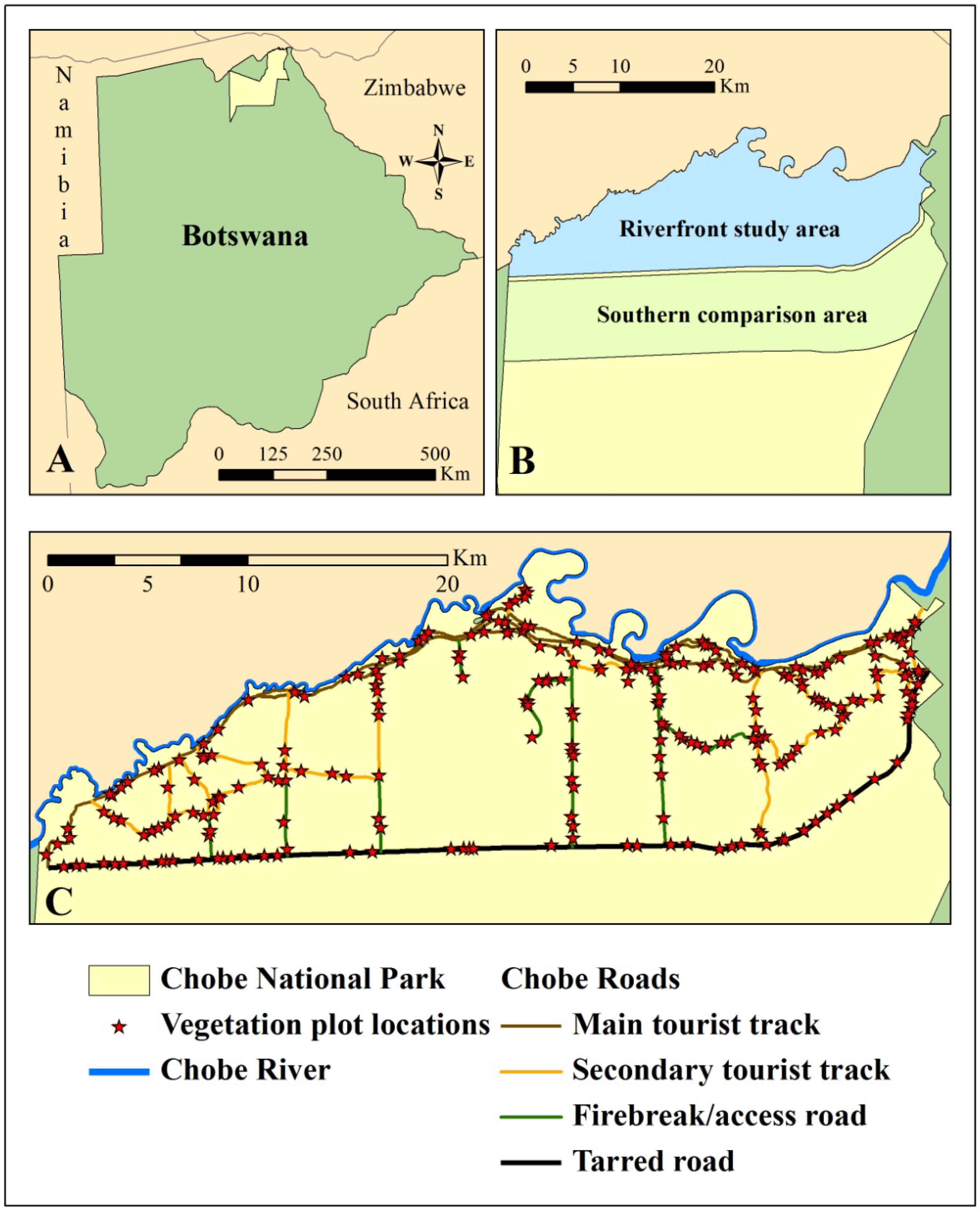
2.1. Study Area
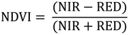
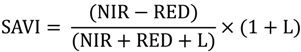
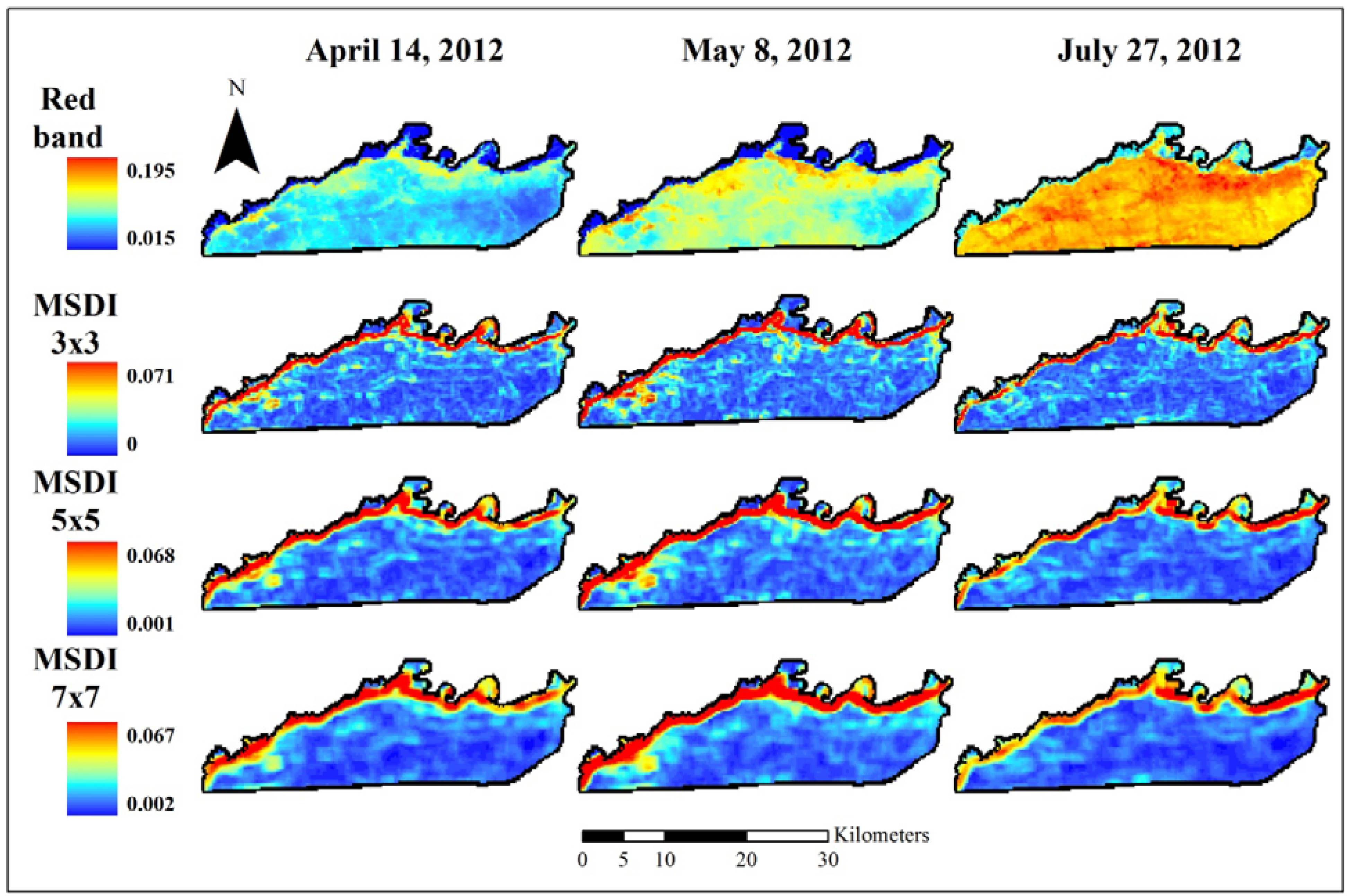
2.2. Remote Sensing Data Preparation and MSDI Calculation


2.3. Coarse Assessment of MSDI
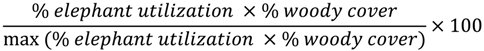
2.4. Fine Assessment of MSDI
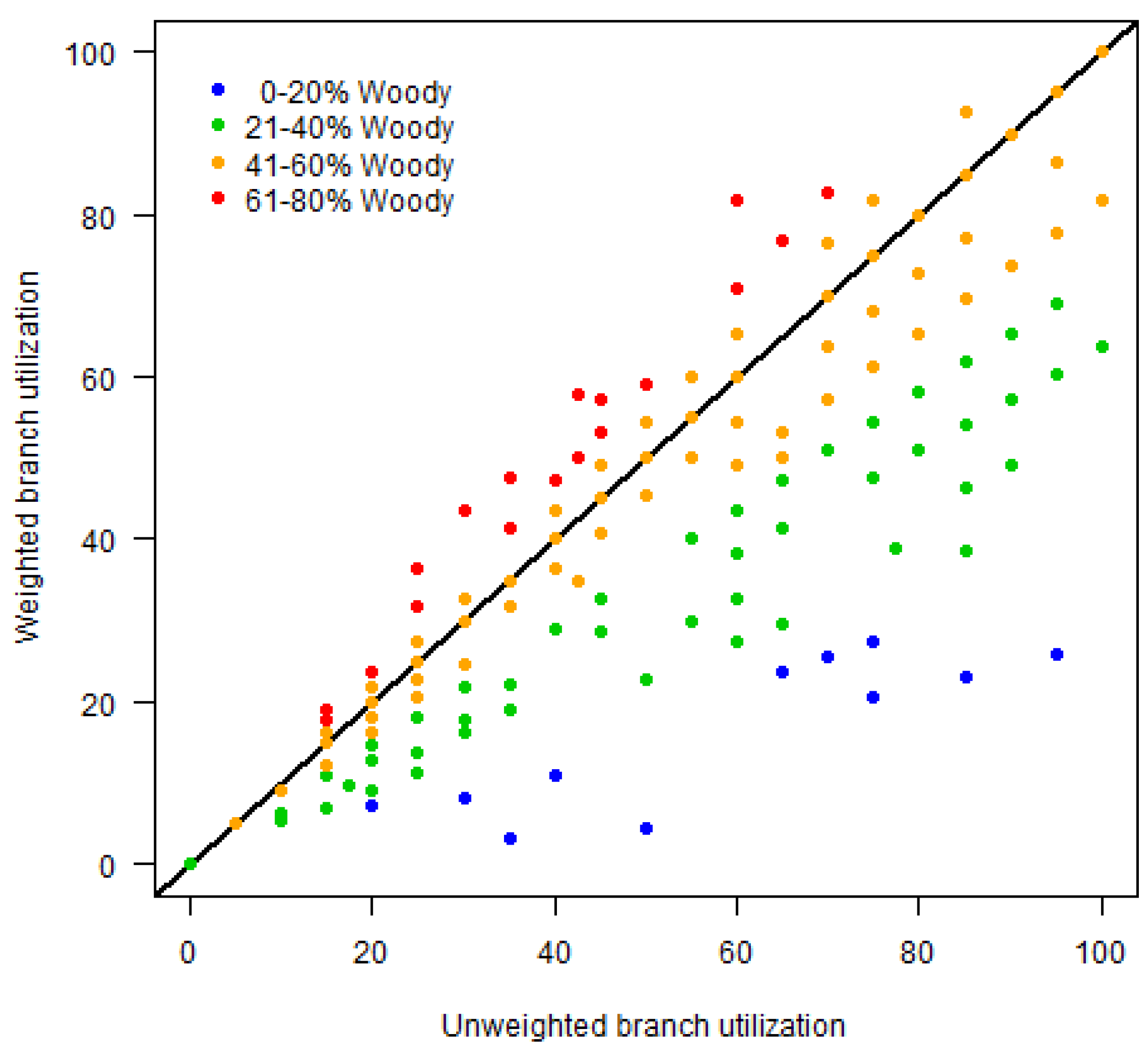
2.4.1. Field Data Collection

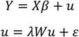
2.4.2. Statistical Analysis
2.4.3. Assessment of Alternative Covariates
3. Results
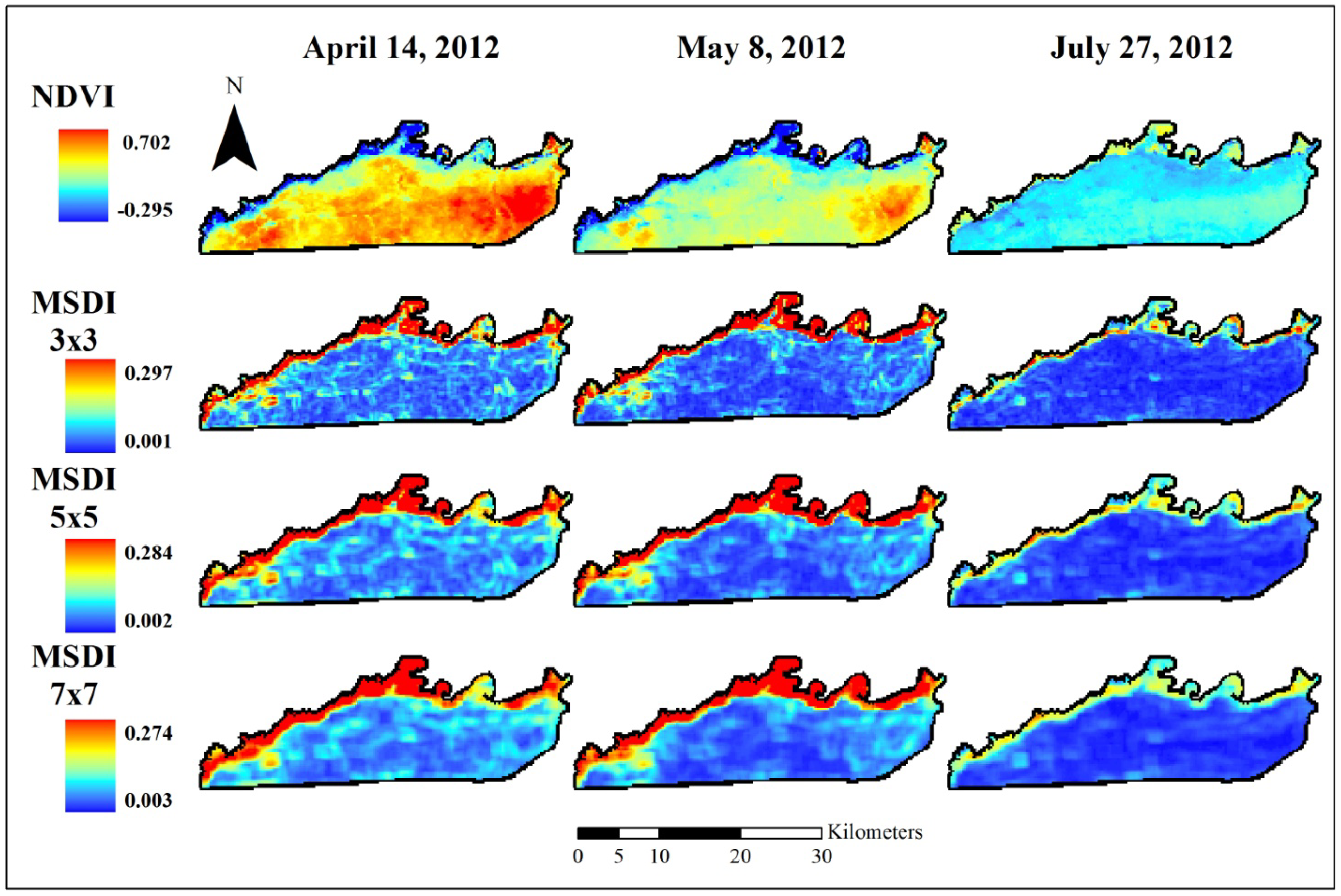
3.1. Coarse Assessment of MSDI
3.2. Fine Assessment of MSDI
3.2.1. Regression Assessment of Elephant Utilization

| Image | Window | Date | Intercept | MSDI | Lambda | RMSE | R2 | ΔAIC | |||
|---|---|---|---|---|---|---|---|---|---|---|---|
| Red | 3 × 3 | 14/4 | 50.120 | (3.857) | −824.476 | (124.373) | 0.631 | (0.101) | 20.69 | 0.22 | 23.1 |
| 8/5 | 49.039 | (3.934) | −601.929 | (88.871) | 0.648 | (0.098) | 20.61 | 0.23 | 24.9 | ||
| 27/7 | 46.934 | (3.549) | −674.380 | (148.144) | 0.575 | (0.112) | 21.59 | 0.16 | 16.7 | ||
| 5 × 5 | 14/4 | 52.748 | (4.388) | −850.280 | (122.238) | 0.673 | (0.093) | 20.51 | 0.24 | 27.6 | |
| 8/5 | 50.096 | (4.170) | −531.774 | (87.233) | 0.653 | (0.097) | 20.91 | 0.21 | 24.9 | ||
| 27/7 | 49.925 | (3.889) | −742.468 | (130.328) | 0.615 | (0.104) | 21.11 | 0.19 | 20.4 | ||
| 7 × 7 | 14/4 | 53.283 | (4.546) | −811.058 | (130.336) | 0.669 | (0.093) | 20.85 | 0.21 | 25.7 | |
| 8/5 | 50.040 | (4.202) | −473.364 | (90.751) | 0.637 | (0.100) | 21.29 | 0.18 | 22.3 | ||
| 27/7 | 50.046 | (4.034) | −674.057 | (128.717) | 0.619 | (0.103) | 21.30 | 0.18 | 20.3 | ||
| NIR | 3 × 3 | 14/4 | 47.391 | (3.531) | −326.513 | (46.806) | 0.616 | (0.104) | 20.55 | 0.24 | 20.6 |
| 8/5 | 47.356 | (3.724) | −282.070 | (40.693) | 0.638 | (0.100) | 20.55 | 0.24 | 23.0 | ||
| 27/7 | 45.927 | (3.338) | −365.119 | (92.122) | 0.541 | (0.118) | 21.83 | 0.14 | 13.5 | ||
| 5 × 5 | 14/4 | 48.374 | (3.919) | −298.169 | (43.662) | 0.651 | (0.097) | 20.59 | 0.23 | 23.6 | |
| 8/5 | 47.707 | (3.903) | −233.403 | (38.227) | 0.642 | (0.099) | 20.92 | 0.21 | 22.8 | ||
| 27/7 | 48.385 | (3.586) | −418.671 | (82.998) | 0.575 | (0.112) | 21.41 | 0.17 | 16.2 | ||
| 7 × 7 | 14/4 | 48.565 | (4.010) | −269.858 | (43.968) | 0.648 | (0.098) | 20.90 | 0.21 | 22.7 | |
| 8/5 | 47.750 | (3.934) | −205.667 | (38.498) | 0.632 | (0.101) | 21.24 | 0.18 | 21.2 | ||
| 27/7 | 48.468 | (3.747) | −386.700 | (83.097) | 0.584 | (0.110) | 21.55 | 0.16 | 16.8 | ||
| NDVI | 3 × 3 | 14/4 | 48.601 | (3.580) | −213.858 | (44.825) | 0.561 | (0.114) | 21.53 | 0.16 | 16.0 |
| 8/5 | 47.277 | (3.482) | −192.491 | (34.795) | 0.586 | (0.110) | 21.21 | 0.19 | 18.0 | ||
| 27/7 | 46.938 | (3.479) | −429.337 | (94.926) | 0.564 | (0.114) | 21.61 | 0.15 | 16.4 | ||
| 5 × 5 | 14/4 | 50.779 | (4.328) | −206.896 | (40.974) | 0.638 | (0.100) | 21.35 | 0.17 | 22.9 | |
| 8/5 | 49.110 | (3.752) | −175.571 | (33.094) | 0.597 | (0.108) | 21.29 | 0.18 | 18.7 | ||
| 27/7 | 49.559 | (3.816) | −427.776 | (76.246) | 0.608 | (0.106) | 21.16 | 0.19 | 21.0 | ||
| 7 × 7 | 14/4 | 50.412 | (4.504) | −175.691 | (40.219) | 0.637 | (0.100) | 21.60 | 0.15 | 21.9 | |
| 8/5 | 49.905 | (4.026) | −164.583 | (31.986) | 0.617 | (0.104) | 21.33 | 0.18 | 19.8 | ||
| 27/7 | 50.220 | (3.941) | −404.006 | (73.008) | 0.614 | (0.104) | 21.18 | 0.19 | 21.3 | ||
| SAVI | 3 × 3 | 14/4 | 48.743 | (3.436) | −318.769 | (52.687) | 0.576 | (0.112) | 21.00 | 0.20 | 17.1 |
| 8/5 | 47.949 | (3.537) | −321.785 | (51.739) | 0.601 | (0.107) | 20.90 | 0.21 | 19.2 | ||
| 27/7 | 44.719 | (3.341) | −415.079 | (145.690) | 0.522 | (0.122) | 22.16 | 0.11 | 12.2 | ||
| 5 × 5 | 14/4 | 49.486 | (3.887) | −275.062 | (48.632) | 0.619 | (0.103) | 21.13 | 0.19 | 20.7 | |
| 8/5 | 48.114 | (3.789) | −255.448 | (48.091) | 0.612 | (0.105) | 21.27 | 0.18 | 19.8 | ||
| 27/7 | 47.986 | (3.618) | −554.728 | (126.871) | 0.562 | (0.114) | 21.67 | 0.15 | 16.1 | ||
| 7 × 7 | 14/4 | 49.351 | (4.045) | −238.349 | (47.728) | 0.621 | (0.103) | 21.39 | 0.17 | 20.4 | |
| 8/5 | 47.926 | (3.884) | −217.275 | (46.835) | 0.608 | (0.105) | 21.53 | 0.16 | 19.1 | ||
| 27/7 | 48.700 | (3.799) | −550.661 | (127.308) | 0.574 | (0.112) | 21.67 | 0.15 | 17.1 | ||
| MSAVI2 | 3 × 3 | 14/4 | 48.834 | (3.410) | −338.572 | (56.729) | 0.569 | (0.113) | 21.04 | 0.20 | 16.4 |
| 8/5 | 48.073 | (3.526) | −350.666 | (56.679) | 0.598 | (0.107) | 20.92 | 0.21 | 18.9 | ||
| 27/7 | 44.804 | (3.333) | −428.316 | (149.076) | 0.519 | (0.122) | 22.15 | 0.11 | 11.9 | ||
| 5 × 5 | 14/4 | 49.652 | (3.851) | −295.497 | (52.541) | 0.612 | (0.105) | 21.15 | 0.19 | 20.0 | |
| 8/5 | 48.106 | (3.776) | −275.033 | (52.561) | 0.609 | (0.105) | 21.31 | 0.18 | 19.5 | ||
| 27/7 | 48.144 | (3.609) | −581.133 | (132.513) | 0.558 | (0.115) | 21.67 | 0.15 | 15.7 | ||
| 7 × 7 | 14/4 | 49.419 | (4.006) | −253.828 | (51.741) | 0.613 | (0.105) | 21.43 | 0.17 | 19.6 | |
| 8/5 | 47.857 | (3.854) | −233.194 | (51.171) | 0.603 | (0.106) | 21.56 | 0.16 | 18.6 | ||
| 27/7 | 48.764 | (3.776) | −573.581 | (132.332) | 0.570 | (0.113) | 21.67 | 0.15 | 16.6 | ||
3.2.2. Kriging Assessment of Elephant Utilization
| Method | Covariate | Window | Date | Variogram | Range | Sill | Nugget | RMSE | R2 |
|---|---|---|---|---|---|---|---|---|---|
| Ordinary | Constant | Spherical | 3,653 | 592 | 251 | 18.85 | 0.36 | ||
| Universal | Red | 3 × 3 | 4/14/2012 | Exponential | 1,314 | 512 | 185 | 18.50 | 0.38 |
| 5/8/2012 | Exponential | 1,342 | 517 | 158 | 18.21 | 0.40 | |||
| 7/27/2012 | Exponential | 1,291 | 552 | 181 | 18.88 | 0.35 | |||
| 5 × 5 | 4/14/2012 | Exponential | 1,400 | 515 | 185 | 18.27 | 0.40 | ||
| 5/8/2012 | Exponential | 1,392 | 531 | 185 | 18.37 | 0.39 | |||
| 7/27/2012 | Exponential | 1,429 | 537 | 189 | 18.45 | 0.38 | |||
| 7 × 7 | 4/14/2012 | Exponential | 1,365 | 527 | 189 | 18.50 | 0.38 | ||
| 5/8/2012 | Exponential | 1,322 | 541 | 187 | 18.65 | 0.37 | |||
| 7/27/2012 | Exponential | 1,369 | 545 | 185 | 18.54 | 0.38 | |||
| NIR | 3 × 3 | 4/14/2012 | Exponential | 1,350 | 506 | 183 | 18.32 | 0.39 | |
| 5/8/2012 | Exponential | 1,390 | 516 | 160 | 18.05 | 0.41 | |||
| 7/27/2012 | Exponential | 1,219 | 557 | 183 | 18.96 | 0.35 | |||
| 5 × 5 | 4/14/2012 | Exponential | 1,497 | 517 | 203 | 18.34 | 0.39 | ||
| 5/8/2012 | Exponential | 1,495 | 533 | 201 | 18.41 | 0.39 | |||
| 7/27/2012 | Exponential | 1,341 | 540 | 194 | 18.59 | 0.37 | |||
| 7 × 7 | 4/14/2012 | Exponential | 1,443 | 527 | 206 | 18.54 | 0.38 | ||
| 5/8/2012 | Exponential | 1,399 | 541 | 202 | 18.66 | 0.37 | |||
| 7/27/2012 | Exponential | 1,264 | 546 | 178 | 18.68 | 0.37 | |||
| NDVI | 3 × 3 | 4/14/2012 | Exponential | 1,243 | 541 | 164 | 18.73 | 0.36 | |
| 5/8/2012 | Exponential | 1,227 | 532 | 134 | 18.26 | 0.40 | |||
| 7/27/2012 | Exponential | 1,194 | 548 | 149 | 18.77 | 0.36 | |||
| 5 × 5 | 4/14/2012 | Exponential | 1,305 | 550 | 167 | 18.64 | 0.37 | ||
| 5/8/2012 | Exponential | 1,321 | 538 | 181 | 18.64 | 0.37 | |||
| 7/27/2012 | Exponential | 1,286 | 532 | 159 | 18.40 | 0.39 | |||
| 7 × 7 | 4/14/2012 | Exponential | 1,276 | 560 | 171 | 18.82 | 0.36 | ||
| 5/8/2012 | Exponential | 1,327 | 542 | 185 | 18.75 | 0.36 | |||
| 7/27/2012 | Exponential | 1,313 | 534 | 174 | 18.44 | 0.38 | |||
| SAVI | 3 × 3 | 4/14/2012 | Exponential | 1,234 | 517 | 170 | 18.52 | 0.38 | |
| 5/8/2012 | Exponential | 1,286 | 522 | 152 | 18.20 | 0.40 | |||
| 7/27/2012 | Exponential | 1,128 | 567 | 166 | 19.05 | 0.34 | |||
| 5 × 5 | 4/14/2012 | Exponential | 1,357 | 533 | 191 | 18.59 | 0.37 | ||
| 5/8/2012 | Exponential | 1,347 | 539 | 190 | 18.62 | 0.37 | |||
| 7/27/2012 | Exponential | 1,199 | 546 | 169 | 18.81 | 0.36 | |||
| 7 × 7 | 4/14/2012 | Exponential | 1,319 | 543 | 190 | 18.74 | 0.36 | ||
| 5/8/2012 | Exponential | 1,304 | 547 | 193 | 18.81 | 0.36 | |||
| 7/27/2012 | Exponential | 1,181 | 547 | 162 | 18.81 | 0.36 | |||
| Universal | MSAVI2 | 3 × 3 | 4/14/2012 | Exponential | 1,215 | 518 | 170 | 18.55 | 0.38 |
| 5/8/2012 | Exponential | 1,276 | 522 | 152 | 18.22 | 0.40 | |||
| 7/27/2012 | Exponential | 1,123 | 566 | 169 | 19.06 | 0.34 | |||
| 5 × 5 | 4/14/2012 | Exponential | 1,347 | 532 | 191 | 18.60 | 0.37 | ||
| 5/8/2012 | Exponential | 1,344 | 540 | 190 | 18.63 | 0.37 | |||
| 7/27/2012 | Exponential | 1,201 | 545 | 174 | 18.81 | 0.36 | |||
| 7 × 7 | 4/14/2012 | Exponential | 1,309 | 543 | 190 | 18.75 | 0.36 | ||
| 5/8/2012 | Exponential | 1,296 | 548 | 193 | 18.81 | 0.36 | |||
| 7/27/2012 | Exponential | 1,160 | 545 | 161 | 18.82 | 0.36 |
3.3. Assessment of Alternative Covariates
4. Discussion
| Image | Window | Date | Long. | Lat. | Elev. | Dist. Road | Dist. River | Flow Acc. | Flow Dir. | Slope | Veg. Class |
|---|---|---|---|---|---|---|---|---|---|---|---|
| Red | 3 × 3 | 14/4 | −0.150 | 0.357 | −0.590 | −0.254 | −0.492 | 0.061 | 0.024 | 0.218 | 0.337 |
| 8/5 | −0.149 | 0.304 | −0.543 | −0.286 | −0.471 | 0.047 | 0.032 | 0.226 | 0.314 | ||
| 27/7 | 0.003 | 0.419 | −0.594 | −0.238 | −0.456 | 0.026 | −0.025 | 0.165 | 0.310 | ||
| 5 × 5 | 14/4 | −0.135 | 0.469 | −0.709 | −0.302 | −0.600 | 0.037 | 0.032 | 0.162 | 0.401 | |
| 8/5 | −0.122 | 0.427 | −0.679 | −0.346 | −0.590 | 0.018 | 0.036 | 0.176 | 0.382 | ||
| 27/7 | −0.013 | 0.513 | −0.700 | −0.299 | −0.568 | 0.000 | −0.001 | 0.170 | 0.376 | ||
| 7 × 7 | 14/4 | −0.118 | 0.523 | −0.769 | −0.329 | −0.664 | 0.036 | 0.027 | 0.141 | 0.438 | |
| 8/5 | −0.114 | 0.471 | −0.739 | −0.364 | −0.653 | 0.013 | 0.037 | 0.153 | 0.414 | ||
| 27/7 | −0.016 | 0.540 | −0.738 | −0.324 | −0.619 | −0.021 | 0.012 | 0.161 | 0.414 | ||
| NIR | 3 × 3 | 14/4 | −0.046 | 0.388 | −0.602 | −0.215 | −0.460 | 0.011 | −0.016 | 0.197 | 0.278 |
| 8/5 | −0.059 | 0.363 | −0.573 | −0.237 | −0.459 | 0.004 | −0.001 | 0.200 | 0.275 | ||
| 27/7 | 0.104 | 0.465 | −0.618 | −0.187 | −0.468 | −0.009 | −0.039 | 0.142 | 0.304 | ||
| 5 × 5 | 14/4 | −0.034 | 0.499 | −0.714 | −0.269 | −0.566 | −0.013 | 0.000 | 0.147 | 0.341 | |
| 8/5 | −0.050 | 0.461 | −0.684 | −0.301 | −0.562 | −0.013 | 0.012 | 0.167 | 0.340 | ||
| 27/7 | 0.107 | 0.538 | −0.688 | −0.254 | −0.554 | −0.012 | −0.008 | 0.168 | 0.356 | ||
| 7 × 7 | 14/4 | −0.044 | 0.528 | −0.751 | −0.284 | −0.616 | −0.019 | 0.007 | 0.130 | 0.369 | |
| 8/5 | −0.060 | 0.497 | −0.731 | −0.316 | −0.620 | −0.017 | 0.020 | 0.148 | 0.376 | ||
| 27/7 | 0.096 | 0.558 | −0.713 | −0.278 | −0.600 | −0.023 | 0.017 | 0.170 | 0.386 | ||
| NDVI | 3 × 3 | 14/4 | −0.105 | 0.412 | −0.642 | −0.187 | −0.505 | 0.053 | −0.020 | 0.129 | 0.332 |
| 8/5 | −0.023 | 0.487 | −0.680 | −0.146 | −0.515 | 0.022 | −0.056 | 0.049 | 0.316 | ||
| 27/7 | −0.058 | 0.364 | −0.595 | −0.169 | −0.434 | −0.010 | −0.071 | 0.124 | 0.263 | ||
| 5 × 5 | 14/4 | −0.121 | 0.484 | −0.707 | −0.252 | −0.590 | 0.034 | 0.015 | 0.116 | 0.377 | |
| 8/5 | −0.017 | 0.551 | −0.746 | −0.224 | −0.597 | 0.004 | −0.025 | 0.090 | 0.358 | ||
| 27/7 | −0.099 | 0.431 | −0.681 | −0.231 | −0.520 | 0.010 | −0.053 | 0.125 | 0.316 | ||
| 7 × 7 | 14/4 | −0.137 | 0.509 | −0.729 | −0.294 | −0.631 | 0.033 | 0.024 | 0.114 | 0.399 | |
| 8/5 | −0.025 | 0.575 | −0.773 | −0.265 | −0.643 | 0.009 | −0.010 | 0.084 | 0.380 | ||
| 27/7 | −0.116 | 0.455 | −0.710 | −0.270 | −0.559 | 0.002 | −0.043 | 0.117 | 0.345 | ||
| SAVI | 3 × 3 | 14/4 | −0.054 | 0.402 | −0.631 | −0.260 | −0.502 | 0.030 | 0.008 | 0.206 | 0.313 |
| 8/5 | −0.029 | 0.430 | −0.649 | −0.261 | −0.529 | 0.023 | 0.011 | 0.180 | 0.316 | ||
| 27/7 | 0.032 | 0.378 | −0.579 | −0.145 | −0.425 | −0.025 | −0.069 | 0.129 | 0.252 | ||
| 5 × 5 | 14/4 | −0.058 | 0.488 | −0.720 | −0.323 | −0.600 | 0.010 | 0.030 | 0.155 | 0.362 | |
| 8/5 | −0.023 | 0.497 | −0.718 | −0.331 | −0.606 | −0.003 | 0.027 | 0.165 | 0.356 | ||
| 27/7 | 0.010 | 0.447 | −0.663 | −0.225 | −0.511 | 0.001 | −0.038 | 0.138 | 0.299 | ||
| 7 × 7 | 14/4 | −0.076 | 0.505 | −0.743 | −0.346 | −0.642 | 0.008 | 0.036 | 0.139 | 0.383 | |
| 8/5 | −0.043 | 0.510 | −0.744 | −0.347 | −0.649 | −0.001 | 0.036 | 0.144 | 0.376 | ||
| 27/7 | 0.001 | 0.470 | −0.687 | −0.254 | −0.543 | −0.002 | −0.023 | 0.139 | 0.323 | ||
| MSAVI2 | 3 × 3 | 14/4 | −0.040 | 0.390 | −0.611 | −0.270 | −0.489 | 0.027 | 0.015 | 0.216 | 0.301 |
| 8/5 | −0.022 | 0.414 | −0.625 | −0.274 | −0.517 | 0.022 | 0.025 | 0.195 | 0.306 | ||
| 27/7 | 0.043 | 0.387 | −0.584 | −0.144 | −0.430 | −0.026 | −0.067 | 0.129 | 0.253 | ||
| 5 × 5 | 14/4 | −0.039 | 0.483 | −0.708 | −0.334 | −0.592 | 0.006 | 0.037 | 0.159 | 0.353 | |
| 8/5 | −0.016 | 0.485 | −0.703 | −0.340 | −0.598 | −0.003 | 0.033 | 0.171 | 0.348 | ||
| 27/7 | 0.025 | 0.458 | −0.667 | −0.226 | −0.514 | 0.001 | −0.036 | 0.142 | 0.301 | ||
| 7 × 7 | 14/4 | −0.057 | 0.499 | −0.732 | −0.356 | −0.635 | 0.006 | 0.041 | 0.142 | 0.374 | |
| 8/5 | −0.034 | 0.500 | −0.731 | −0.354 | −0.642 | −0.001 | 0.041 | 0.147 | 0.367 | ||
| 27/7 | 0.016 | 0.476 | −0.688 | −0.253 | −0.544 | −0.002 | −0.019 | 0.141 | 0.322 |
| Image | Window | Date | Long. | Lat. | Elev. | Dist. Road | Dist. River | Flow Acc. | Flow Dir. | Slope | Veg. Class |
|---|---|---|---|---|---|---|---|---|---|---|---|
| Red | 3 × 3 | 14/4 | −0.346 | −0.010 | −0.366 | −0.185 | −0.342 | 0.062 | −0.028 | 0.031 | 0.018 |
| 8/5 | −0.384 | −0.059 | −0.314 | −0.110 | −0.383 | −0.026 | −0.034 | 0.019 | −0.014 | ||
| 27/7 | −0.300 | 0.042 | −0.218 | −0.136 | −0.321 | −0.022 | −0.035 | 0.037 | −0.006 | ||
| 5 × 5 | 14/4 | −0.450 | −0.005 | −0.416 | −0.182 | −0.449 | 0.013 | −0.054 | 0.007 | 0.010 | |
| 8/5 | −0.477 | −0.040 | −0.377 | −0.152 | −0.479 | −0.033 | −0.058 | 0.010 | −0.018 | ||
| 27/7 | −0.395 | 0.096 | −0.310 | −0.202 | −0.427 | −0.036 | −0.027 | −0.021 | 0.010 | ||
| 7 × 7 | 14/4 | −0.491 | −0.017 | −0.444 | −0.172 | −0.485 | −0.011 | −0.072 | 0.005 | 0.011 | |
| 8/5 | −0.526 | −0.039 | −0.401 | −0.140 | −0.525 | −0.054 | −0.088 | 0.005 | −0.031 | ||
| 27/7 | −0.485 | 0.078 | −0.366 | −0.230 | −0.517 | −0.062 | −0.056 | −0.027 | −0.004 | ||
| NIR | 3 × 3 | 14/4 | −0.285 | −0.093 | −0.210 | −0.055 | −0.270 | −0.031 | −0.028 | −0.038 | 0.027 |
| 8/5 | −0.296 | −0.100 | −0.233 | −0.071 | −0.291 | −0.065 | −0.033 | −0.006 | 0.017 | ||
| 27/7 | 0.135 | 0.248 | −0.120 | −0.214 | 0.108 | −0.035 | 0.070 | 0.092 | 0.121 | ||
| 5 × 5 | 14/4 | −0.422 | −0.082 | −0.296 | −0.093 | −0.413 | −0.067 | −0.071 | −0.023 | 0.029 | |
| 8/5 | −0.430 | −0.113 | −0.307 | −0.122 | −0.428 | −0.062 | −0.083 | 0.001 | 0.036 | ||
| 27/7 | 0.116 | 0.382 | −0.167 | −0.268 | 0.068 | −0.016 | 0.060 | 0.072 | 0.165 | ||
| 7 × 7 | 14/4 | −0.489 | −0.082 | −0.345 | −0.121 | −0.478 | −0.062 | −0.100 | −0.007 | 0.015 | |
| 8/5 | −0.506 | −0.120 | −0.342 | −0.122 | −0.501 | −0.084 | −0.086 | 0.002 | 0.035 | ||
| 27/7 | 0.095 | 0.432 | −0.181 | −0.278 | 0.040 | −0.017 | 0.033 | 0.030 | 0.144 | ||
| NDVI | 3 × 3 | 14/4 | −0.101 | 0.292 | −0.357 | −0.259 | −0.129 | 0.119 | 0.000 | 0.076 | 0.063 |
| 8/5 | −0.203 | 0.215 | −0.307 | −0.238 | −0.235 | 0.060 | 0.022 | 0.064 | −0.002 | ||
| 27/7 | −0.186 | 0.101 | −0.218 | −0.190 | −0.212 | 0.019 | −0.020 | 0.048 | 0.010 | ||
| 5 × 5 | 14/4 | −0.141 | 0.344 | −0.396 | −0.266 | −0.172 | 0.073 | −0.002 | 0.035 | 0.079 | |
| 8/5 | −0.229 | 0.264 | −0.341 | −0.255 | −0.264 | 0.036 | −0.003 | 0.018 | −0.021 | ||
| 27/7 | −0.272 | 0.104 | −0.290 | −0.232 | −0.303 | −0.008 | −0.028 | 0.010 | 0.019 | ||
| 7 × 7 | 14/4 | −0.115 | 0.357 | −0.388 | −0.240 | −0.138 | 0.050 | −0.005 | 0.022 | 0.084 | |
| 8/5 | −0.217 | 0.293 | −0.338 | −0.251 | −0.254 | 0.027 | −0.021 | 0.014 | −0.034 | ||
| 27/7 | −0.340 | 0.118 | −0.353 | −0.277 | −0.370 | −0.017 | −0.033 | −0.009 | 0.008 | ||
| SAVI | 3 × 3 | 14/4 | 0.043 | 0.306 | −0.239 | −0.177 | 0.015 | 0.160 | −0.019 | 0.072 | 0.074 |
| 8/5 | −0.092 | 0.249 | −0.253 | −0.245 | −0.121 | 0.135 | 0.012 | 0.070 | 0.029 | ||
| 27/7 | −0.102 | 0.089 | −0.204 | −0.169 | −0.116 | 0.012 | −0.009 | 0.058 | 0.044 | ||
| 5 × 5 | 14/4 | 0.027 | 0.391 | −0.299 | −0.211 | 0.001 | 0.101 | −0.019 | 0.042 | 0.097 | |
| 8/5 | −0.083 | 0.318 | −0.290 | −0.283 | −0.115 | 0.087 | 0.015 | 0.007 | 0.022 | ||
| 27/7 | −0.133 | 0.116 | −0.247 | −0.211 | −0.153 | −0.016 | −0.008 | 0.034 | 0.068 | ||
| 7 × 7 | 14/4 | 0.051 | 0.406 | −0.295 | −0.170 | 0.035 | 0.068 | −0.011 | 0.031 | 0.099 | |
| 8/5 | −0.051 | 0.354 | −0.277 | −0.268 | −0.084 | 0.071 | −0.010 | 0.005 | 0.005 | ||
| 27/7 | −0.158 | 0.151 | −0.293 | −0.252 | −0.176 | −0.023 | −0.014 | 0.014 | 0.059 | ||
| MSAVI2 | 3 × 3 | 14/4 | 0.068 | 0.326 | −0.246 | −0.174 | 0.041 | 0.135 | −0.010 | 0.079 | 0.075 |
| 8/5 | −0.044 | 0.262 | −0.237 | −0.240 | −0.073 | 0.140 | 0.021 | 0.051 | 0.037 | ||
| 27/7 | −0.055 | 0.112 | −0.206 | −0.171 | −0.068 | 0.017 | 0.013 | 0.075 | 0.064 | ||
| 5 × 5 | 14/4 | 0.066 | 0.405 | −0.275 | −0.202 | 0.042 | 0.084 | −0.030 | 0.046 | 0.102 | |
| 8/5 | −0.019 | 0.337 | −0.255 | −0.285 | −0.051 | 0.082 | 0.011 | 0.006 | 0.050 | ||
| 27/7 | −0.080 | 0.140 | −0.239 | −0.221 | −0.097 | −0.005 | 0.007 | 0.050 | 0.092 | ||
| 7 × 7 | 14/4 | 0.074 | 0.428 | −0.296 | −0.173 | 0.058 | 0.055 | −0.012 | 0.041 | 0.119 | |
| 8/5 | 0.014 | 0.374 | −0.246 | −0.272 | −0.016 | 0.083 | −0.004 | 0.004 | 0.031 | ||
| 27/7 | −0.100 | 0.175 | −0.280 | −0.240 | −0.116 | −0.028 | −0.005 | 0.024 | 0.085 |

5. Conclusions
Acknowledgments
Author Contributions
Conflicts of Interest
References
- Scholes, R.J.; Archer, S.R. Tree-grass interactions in Savannas. Annu. Rev. Ecol. Syst. 1997, 28, 517–544. [Google Scholar] [CrossRef]
- Sankaran, M.; Hanan, N.P.; Scholes, R.J.; Ratnam, J.; Augustine, D.J.; Cade, B.S.; Gignoux, J.; Higgins, S.I.; Le Roux, X.; Ludwig, F.; et al. Determinants of woody cover in African savannas. Nature 2005, 438, 846–849. [Google Scholar] [CrossRef]
- Skarpe, C. Dynamics of savanna ecosystems. J. Veg. Sci. 1992, 3, 293–300. [Google Scholar] [CrossRef]
- Loarie, S.R.; van Aarde, R.J.; Pimm, S.L. Elephant seasonal vegetation preferences across dry and wet savannas. Biol. Conserv. 2009, 142, 3099–3107. [Google Scholar] [CrossRef]
- Weltzin, J.F.; Coughenour, M.B. Savanna tree influence on understory vegetation and soil nutrients in northwestern Kenya. J. Veg. Sci. 1990, 1, 325–334. [Google Scholar] [CrossRef]
- Belsky, A.J. Influences of trees on savanna productivity: Tests of shade, nutrients, and tree-grass competition. Ecology 1994, 75, 922–932. [Google Scholar] [CrossRef]
- Sala, O.E.; Chapin, F.S., III; Armesto, J.J.; Berlow, E.; Bloomfield, J.; Dirzo, R.; Huber-Sanwald, E.; Huenneke, L.F.; Jackson, R.B.; Kinzig, A.; et al. Global biodiversity scenarios for the year 2100. Science 2000, 287, 1770–1774. [Google Scholar] [CrossRef]
- Desanker, P.V.; Justice, C.O. Africa and global climate change: Critical issues and suggestions for further research and integrated assessment modeling. Clim. Res. 2001, 17, 93–103. [Google Scholar] [CrossRef]
- Bell, R.H.V. The Effect of Soil Nutrient Availability on Community Structure in African Ecosystems. In Ecology of Tropical Savannas; Huntley, B.J., Walker, B.H., Eds.; Springer-Verlag: Berlin, Germany, 1982; pp. 193–216. [Google Scholar]
- Olff, H.; Ritchie, M.E.; Prins, H.H.T. Global environmental controls of diversity in large herbivores. Nature 2002, 415, 901–904. [Google Scholar] [CrossRef]
- Staver, A.C.; Archibald, S.; Levin, S.A. The global extent and determinants of savanna and forest as alternative biome states. Science 2011, 334, 230–232. [Google Scholar] [CrossRef]
- Staver, A.C.; Archibald, S.; Levin, S.A. Tree cover in Sub-Saharan Africa: Rainfall and fire constrain forest and savanna as alternative stable states. Ecology 2011, 92, 1063–1072. [Google Scholar] [CrossRef]
- Turner, B.L.; Skole, D.; Sanderson, S.; Fischer, G.; Fresco, L.; Leemans, R. Land-Use and Land-Cover Change. Science/Research Plan; IGBP Report No. 35 and HDP Report No. 7; International Geosphere-Biosphere Programme/Human Dimensions of Global Environmental Change Programme: Stockholm, Sweden/Geneva, Switzerland, 1995. [Google Scholar]
- Geist, H.J.; Lambin, E.F.; Rindfuss, R.R. Land Use and Land Cover Change. In Land-Use and Land-Cover Change: Local Processes and Global Impacts; Springer: New York, NY, USA, 2006; pp. 1–8. [Google Scholar]
- Cumming, D.H. The Influence of Large Herbivores on Savanna Structure in Africa. In Ecology of Tropical Savannas; Huntley, B.J., Walker, B.H., Eds.; Springer-Verlag: Berlin, Germany, 1982; pp. 217–245. [Google Scholar]
- Beuchner, H.K.; Dawkins, H.C. Vegetation change induced by elephants and fire in Murchison Falls National Park, Uganda. Ecology 1961, 42, 752–766. [Google Scholar] [CrossRef]
- Laws, R.M. Elephants as agents of habitat and landscape change in East Africa. Oikos 1970, 21, 1–15. [Google Scholar]
- Barnes, R.F.W. Effects of elephant browsing on woodlands in a Tanzanian National Park: Measurements, models and management. J. Appl. Ecol. 1983, 20, 521–540. [Google Scholar] [CrossRef]
- Goheen, J.R.; Keesing, F.; Allan, B.; Ogada, D.; Ostfeld, R. Net effects of large mammals on Acacia seedling survival in an African savanna. Ecology 2004, 85, 1555–1561. [Google Scholar] [CrossRef]
- Kerley, G.I.H.; Landman, M.; Kruger, L.; Owen-Smith, N.; Balfour, D.; de Boer, W.; Gaylard, A.; Lindsay, K.; Slotow, R. Effects of Elephants on Ecosystems and Biodiversity. In Elephant Management: A Scientific Assessment of South Africa; Scholes, R.J., Mennell, K.G., Eds.; Witwatersrand University Press: Johannesburg, South Africa, 2008; pp. 146–205. [Google Scholar]
- Paine, R.T. A note on trophic complexity and community stability. Am. Nat. 1969, 103, 91–93. [Google Scholar]
- Holdo, R.M. Elephants, fire, and frost can determine community structure and composition in Kalahari woodlands. Ecol. Appl. 2007, 17, 558–568. [Google Scholar] [CrossRef]
- Norton-Griffiths, M. The Influence of Grazing, Browsing, and Fire on the Vegetation Dynamics of the Serengeti. In Serengeti: Dynamics of an Ecosystem; Sinclair, A.R.E., Norton-Griffiths, M., Eds.; University of Chicago Press: Chicago, IL, USA, 1979; pp. 310–351. [Google Scholar]
- Kerley, G.I.H.; Landman, M. The impacts of elephants on biodiversity in the Eastern Cape subtropical thickets. S. Afr. J. Sci. 2006, 102, 395–402. [Google Scholar]
- United Nations Environment Programme (UNEP); Convention on International Trade in Endangered Species of Wild Fauna and Flora (CITES); International Union for Conservation of Nature (IUCN); TRAFFIC. Elephants in the Dust—The African Elephant Crisis; A Rapid Response Assessment; United Nations Environment Programme/GRID-Arendal. Available online: http://www.grida.no/publications/rr/elephants/ (accessed on 22 April 2013).
- Glover, J. The elephant problem at Tsavo. Afr. J. Ecol. 1963, 1, 30–39. [Google Scholar] [CrossRef]
- Barnes, R.F.W. The elephant problem in Ruaha National Park, Tanzania. Biol. Conserv. 1983, 26, 127–148. [Google Scholar] [CrossRef]
- Valeix, M.; Fritz, H.; Dubois, S.; Kanengoni, K.; Alleaume, S.; Said, S. Vegetation structure and ungulate abundance over a period of increasing elephant abundance in Hwange National Park, Zimbabwe. J. Trop. Ecol. 2007, 23, 87–93. [Google Scholar] [CrossRef]
- Blanc, J.J.; Barnes, R.F.W.; Craig, G.C.; Dublin, H.T.; Thouless, C.R.; Douglas-Hamilton, I.; Hart, J.A. African Elephant Status Report 2007: An Update from the African Elephant Database; Occasional Paper Series of the IUCN Species Survival Commission, No. 33; IUCN/SSC African Elephant Specialist Group, International Union for Conservation of Nature (IUCN): Gland, Switzerland, 2007. [Google Scholar]
- Blignaut, J.; de Wit, M.; Barnes, J. The Economic Value of Elephants. In Elephant Management: A Scientific Assessment of South Africa; Scholes, R.J., Mennell, K.G., Eds.; Witwatersrand University Press: Johannesburg, South Africa, 2008; pp. 446–476. [Google Scholar]
- Thouless, C.R. Conflict between humans and elephants on private land in northern Kenya. Oryx 1994, 28, 119–127. [Google Scholar] [CrossRef]
- Hoare, R.E. Determinants of human-elephant conflict in a land-use mosaic. J. Appl. Ecol. 1999, 36, 689–700. [Google Scholar] [CrossRef]
- Hoare, R.E. African elephants and humans in conflict: The outlook for co-existence. Oryx 2000, 34, 34–38. [Google Scholar]
- Prins, H.H.T. Chapter 6/7; Competition for Food/Patch Selection Predators and Grazing by Rule of Thumb. In Ecology and Behaviour of the African Buffalo: Social Inequality and Decision Making; Chapman & Hall: London, UK, 1996; pp. 154–203. [Google Scholar]
- Skarpe, C.; Aarrestad, P.A.; Andreassen, H.P.; Dhillion, S.S.; Dimakatso, T.; du Toit, J.T.; Duncan; Halley, J.; Hytteborn, H.; Makhabu, S.; Marl, M.; et al. The return of the giants: Ecological effects of an increasing elephant population. Ambio 2004, 33, 276–282. [Google Scholar]
- Inamdar, A. The Ecological Consequences of Elephant Depletion. Ph.D. Thesis, University of Cambridge, Cambridge, UK, 1996. [Google Scholar]
- Dipotso, F.M.; Skarpe, C.; Kelaeditse, L.; Ramotadima, M. Chobe bushbuck in an elephant-impacted habitat along the Chobe River. Afr. Zool. 2007, 42, 261–267. [Google Scholar] [CrossRef]
- Western, D.; Gichohi, H. Segregation effects and the impoverishment of savanna parks: The case for ecosystem viability analysis. Afr. J. Ecol. 1993, 31, 269–281. [Google Scholar] [CrossRef]
- Rutina, L.P.; Moe, S.R.; Swenson, J.E. Elephant Loxodonta africana driven woodland conversion to shrubland improves dry-season browse availability for impalas Aepyceros melampus. Wildl. Biol. 2005, 11, 207–213. [Google Scholar] [CrossRef]
- Makhabu, S.W.; Skarpe, C.; Hytteborn, H. Elephant impact on shoot distribution on trees and on rebrowsing by smaller browsers. Acta Oecol. 2006, 30, 136–146. [Google Scholar] [CrossRef]
- Valeix, M.; Fritz, H.; Sabatier, R.; Murindagomo, F.; Cumming, D.; Duncan, P. Elephant-induced structural changes in the vegetation and habitat selection by large herbivores in an African savanna. Biol. Conserv. 2011, 144, 902–912. [Google Scholar] [CrossRef]
- Tanser, F.C.; Palmer, A.R. The application of a remotely-sensed diversity index to monitor degradation patterns in a semi-arid, heterogeneous, South African landscape. J. Arid Environ. 1999, 43, 477–484. [Google Scholar] [CrossRef]
- Schlesinger, W.H.; Reynolds, J.F.; Cunningham, G.L.; Huenneke, L.F.; Jarrell, W.M.; Virginia, R.A.; Whitford, W.G. Biological feedbacks in global desertification. Science 1990, 247, 1043–1048. [Google Scholar]
- Jafari, R.; Lewis, M.M.; Ostendorf, B. An image-based diversity index for assessing land degredation in an arid environment in South Australia. J. Arid Environ. 2008, 72, 1282–1293. [Google Scholar] [CrossRef]
- Pickup, G.; Chewings, V.H. Forecasting patterns of erosion in arid lands from Landsat MSS data. Int. J. Remote Sens. 1988, 9, 69–84. [Google Scholar] [CrossRef]
- Jensen, J.R. Chapter 8: Image Enhancement. In Introductory Digital Image Processing: A Remote Sensing Perspective, 3rd ed.; Pearson Education, Inc.: Upper Saddle River, NJ, USA, 2005; pp. 301–322. [Google Scholar]
- Knipling, E.B. Physical and physiological basis for the reflectance of visible and near-infrared radiation from vegetation. Remote Sens. Environ. 1970, 1, 155–159. [Google Scholar] [CrossRef]
- Tucker, C.J. Red and photographic infrared linear combinations for monitoring vegetation. Remote Sens. Environ. 1979, 8, 127–150. [Google Scholar] [CrossRef]
- Chavez, P.S., Jr.; MacKinnon, D.J. Automatic detection of vegetation changes in the southwestern United States using remotely sensed images. Photogramm. Eng. Remote Sens. 1994, 60, 571–583. [Google Scholar]
- Horler, D.N.; Dockray, M.; Barber, J. The red edge of plant leaf reflectance. Int. J. Remote Sens. 1983, 4, 273–288. [Google Scholar] [CrossRef]
- Huete, A.R. A soil-adjusted vegetation index (SAVI). Remote Sens. Environ. 1988, 25, 295–309. [Google Scholar]
- Huete, A.R.; Liu, H.Q.; Batchily, K.; van Leeuwen, W. A comparison of vegetation indices over a global set of TM images for EOS-MODIS. Remote Sens. Environ. 1997, 59, 440–451. [Google Scholar]
- Huete, A.R.; Didan, K.; Miura, T.; Rodriguez, E.P.; Gao, X.; Ferreira, L.G. Overview of the radiometric and biophysical performance of the MODIS vegetation indices. Remote Sens. Environ. 2002, 83, 195–213. [Google Scholar]
- Loveland, T.R.; Reed, B.C.; Brown, J.L.; Ohlen, D.O.; Zhu, Z.; Yang, L.; Merchant, J.W. Development of a global land cover characteristics database and IGBP DISCover from 1 km AVHRR data. Int. J. Remote Sens. 2000, 21, 1303–1330. [Google Scholar] [CrossRef]
- Ecosystem Function in Savannas: Measurement and Modeling at Landscape to Global Scales; Hill, M.; Hanan, N.P. (Eds.) CRC Press: Boca Raton, FL, USA, 2011.
- Archibald, S.; Scholes, R.J. Leaf green-up in a semi-arid African savanna—Separating tree and grass responses to environmental cues. J. Veg. Sci. 2007, 18, 583–594. [Google Scholar]
- Fensholt, R.; Sandholt, I.; Stisen, S. Evaluating MODIS, MERIS, and VEGETATION vegetation indices using in situ measurements in a semiarid environment. IEEE Trans. Geosci. Remote Sens. 2006, 44, 1774–1786. [Google Scholar] [CrossRef]
- Duffy, J.P.; Pettorelli, N. Exploring the relationship between NDVI and African elephant population density in protected areas. Afr. J. Ecol. 2013, 50, 455–463. [Google Scholar] [CrossRef]
- Nellis, M.D.; Lulla, K.; Briggs, J.M.; Bussing, C.E. Interfacing geographic information systems and space shuttle photography for monitoring elephant impact in Botswana. Pap. Proc. Appl. Geogr. Conf. 1990, 13, 10–15. [Google Scholar]
- Robinson, J.A.; Lulla, K.P.; Kashiwagi, M.; Suzuki, M.; Nellis, M.D.; Bussing, C.E.; Long, W.J.L.; McKenzie, L.J. Conservation applications of astronaut photographs of earth: Tidal-flat loss (Japan), elephant effects on vegetation (Botswana), and seagrass and mangrove monitoring (Australia). Conserv. Biol. 2001, 15, 876–884. [Google Scholar] [CrossRef]
- Campbell, A.C. The national park and reserve system in Botswana. Biol. Conserv. 1973, 5, 7–14. [Google Scholar] [CrossRef]
- Cushman, S.A.; Chase, M.; Griffin, C. Elephants in space and time. Oikos 2005, 109, 331–341. [Google Scholar] [CrossRef]
- Child, G. Wildlife utilization and management in Botswana. Biol. Conserv. 1970, 3, 18–22. [Google Scholar] [CrossRef]
- Mosugelo, D.K.; Moe, S.R.; Ringrose, S.; Nellemann, C. Vegetation changes during a 36-year period in northern Chobe National Park, Botswana. Afr. J. Ecol. 2002, 40, 232–240. [Google Scholar] [CrossRef]
- Fullman, T.J.; Child, B. Water distribution at local and landscape scales affects tree utilization by elephants in Chobe National Park, Botswana. Afr. J. Ecol. 2013, 51, 235–243. [Google Scholar] [CrossRef]
- Reich, P.B.; Borchert, R. Water stress and tree phenology in a tropical dry forest in the lowlands of Costa Rica. J. Ecol. 1984, 72, 61–74. [Google Scholar] [CrossRef]
- Borchert, R. Soil and stem water storage determine phenology and distribution of tropical dry forest trees. Ecology 1994, 75, 1437–1449. [Google Scholar] [CrossRef]
- Borchert, R. Climatic periodicity, phenology and cambium activity in dry forest trees. IAWA J. 1999, 20, 239–247. [Google Scholar]
- Shisanya, C.A.; Recha, C.; Anyamba, A. rainfall variability and its impacts on NDVI in arid and semi-arid lands of Kenya. Int. J. Geosci. 2011, 2, 36–47. [Google Scholar] [CrossRef]
- Food and Agriculture Organization of the United Nations (FAO); International Institute for Applied Systems Analysis (IIASA); International Soil Reference and Information Centre (ISRIC); Institute of Soil Science-Chinese Academy of Sciences (ISSCAS); Joint Research Centre of the European Commission (JRC). Harmonized World Soil Database (Version 1.2); FAO/IIASA: Rome, Italy/Laxenburg, Austria, 2012. [Google Scholar]
- Child, G. An Ecological Survey of Northeastern Botswana; FAO #TA2563; Food and Agriculture Organization of the United Nations (FAO): Rome, Italy, 1968. [Google Scholar]
- Herremans, M.; Herremans-Tonnoeyr, D. Land use and the conservation status of raptors in Botswana. Biol. Conserv. 2000, 94, 31–41. [Google Scholar] [CrossRef]
- Gibson, D.S.C.; Craig, G.C.; Masogo, R.M. Trends of the elephant population in northern Botswana from aerial survey data. Pachyderm 1998, 25, 14–27. [Google Scholar]
- Barnes, M.E. Effects of large herbivores and fire on the regeneration of Acacia erioloba woodlands in Chobe National Park, Botswana. Afr. J. Ecol. 2001, 39, 340–350. [Google Scholar] [CrossRef]
- Moe, S.R.; Rutina, L.P.; Hytteborn, H.; du Toit, J.T. What controls woodland regeneration after elephants have killed the big trees? J. Appl. Ecol. 2009, 46, 223–230. [Google Scholar] [CrossRef]
- Peace Parks Foundation: The Global Solution. Available online: http://www.peaceparks.org/ (accessed on 17 September 2013).
- Kavango-Zambezi Transfrontier Conservation Area. Available online: http://www.kavangozambezi.org/ (accessed on 17 September 2013).
- Van Aarde, R.J.; Jackson, T.P.; Ferreira, S.M. Conservation science and elephant management in southern Africa. S. Afr. J. Sci. 2006, 102, 385–388. [Google Scholar]
- Van Aarde, R.J.; Jackson, T.P. Megaparks for meapopulations: Addressing the causes of locally high elephant numbers in southern Africa. Biol. Conserv. 2007, 134, 289–297. [Google Scholar] [CrossRef]
- USGS. LP DAAC Data Pool. Available online: https://lpdaac.usgs.gov/get_data/data_pool (accessed on 11 September 2012).
- USGS. LP DAAC MODIS Reprojection Tool. Available online: https://lpdaac.usgs.gov/tools/modis_reprojection_tool (accessed on 11 September 2012).
- Graetz, R.D.; Pech, R.R.; Davis, A.W. The assessment and monitoring of sparsely vegetated rangelands using calibrated Landsat data. Int. J. Remote Sens. 1988, 9, 1201–1222. [Google Scholar] [CrossRef]
- McNaughton, S.J.; Oesterheld, M.; Frank, D.A.; Williams, K.J. Ecosystem-level patterns of primary productivity and herbivory in terrestrial habitats. Nature 1989, 341, 142–144. [Google Scholar] [CrossRef]
- Chapin, F.S., III; Bret-Harte, M.S.; Hobbie, S.A.; Zhong, H. Plant functional types as predictors of transient responses of arctic vegetation to global change. J. Veg. Sci. 1996, 7, 347–358. [Google Scholar] [CrossRef]
- Holm, A.M.; Watson, I.W.; Loneragan, W.A.; Adams, M.A. Loss of patch-scale heterogeneity on primary productivity and rainfall-use efficiency in Western Australia. Basic Appl. Ecol. 2003, 4, 569–578. [Google Scholar] [CrossRef]
- Glenn, E.P.; Huete, A.R.; Nagler, P.L.; Nelson, S.G. Relationship between remotely-sensed vegetation indices, canopy attributes and plant physiological processes: What vegetation indices can and cannot tell us about the landscape. Sensors 2008, 8, 2136–2160. [Google Scholar] [CrossRef]
- Huete, A.; Justice, C.; van Leeuwen, W. MODIS Vegetation Index (MOD 13): Algorithm Theoretical Basis Document. Version 3; USGS Land Process Distributed Active Archive Center, 1999. Available online: http://modis.gsfc.nasa.gov/data/atbd/atbd_mod13.pdf (accessed on 4 December 2012).
- Pettorelli, N.; Ryan, S.; Mueller, T.; Bunnefeld, N.; Jędrzejewska, B.; Lima, M.; Kausrud, K. The Normalized Difference Vegetation Index (NDVI): Unforeseen successes in animal ecology. Clim. Res. 2011, 46, 15–27. [Google Scholar] [CrossRef]
- Huete, A.R.; Jackson, R.D. Suitability of spectral indices for evaluating vegetation characteristics on arid rangelands. Remote Sens. Environ. 1987, 23, 213–232. [Google Scholar] [CrossRef]
- Huete, A.R.; Jackson, R.D. Soil and atmosphere influences on the spectra of partial canopies. Remote Sens. Environ. 1988, 25, 89–105. [Google Scholar] [CrossRef]
- Qi, J.; Kerr, Y.; Chehbouni, A. External Factor Consideration in Vegetation Index Development. In Proceedings of the 6th International Symposium on Physical Measurements and Signatures in Remote Sensing, Val d’Isere, France, 17–21 January 1994; pp. 723–730.
- Hijmans, R.J.; van Etten, J. Raster: Geographic Data Analysis and Modeling, R Package Version 2.0-31; 2012. Available online: http://CRAN.R-project.org/package=raster (accessed on 27 March 2012).
- R Core Team. R: A Language and Environment for Statistical Computing; R Foundation for Statistical Computing: Vienna, Austria, 2012. Available online: http://www.R-project.org (accessed on 9 March 2012).
- Fullman, T.J. Spatial Dynamics of Elephant Impacts on Trees in Chobe National Park, Botswana. M.Sc. Thesis, University of Florida, Gainesville, FL, USA, 2009. [Google Scholar]
- Guldemond, R.; van Aarde, R. A meta-analysis of the impact of African elephants on savanna vegetation. J. Wildl. Manag. 2008, 72, 892–899. [Google Scholar]
- Young, T.P.; Palmer, T.M.; Gadd, M.E. Competition and compensation among cattle, zebras, and elephants in a semi-arid savanna in Laikipia, Kenya. Biol. Conserv. 2005, 122, 351–359. [Google Scholar] [CrossRef]
- Fuller, T.K. Do pellet counts index white-tailed deer numbers and population change? J. Wildl. Manag. 1991, 55, 393–396. [Google Scholar]
- Barnes, R.F.W. How reliable are dung counts for estimating elephant numbers? Afr. J. Ecol. 2001, 39, 1–9. [Google Scholar]
- Odén, A.; Wedel, H. Arguments for Fisher’s permutation test. Ann. Stat. 1975, 3, 518–520. [Google Scholar] [CrossRef]
- Ruxton, G.D. The unequal variance t-test is an underused alternative to Student’s t-test and the Mann-Whitney U test. Behav. Ecol. 2006, 17, 688–690. [Google Scholar] [CrossRef]
- Hijmans, R.J.; Phillips, S.; Leathwick, J.; Elith, J. Dismo: Species Distribution Modeling, R Package Version 0.7-23; 2012. Available online: http://CRAN.R-project.org/package=dismo (accessed on 9 March 2012).
- Nellemann, C.; Moe, S.R.; Rutina, L.P. Links between terrain characteristics and forage patterns of elephants (Loxodonta africana) in northern Botswana. J. Trop. Ecol. 2002, 18, 835–844. [Google Scholar]
- Moran, P.A.P. Notes on continuous stochastic phenomena. Biometrika 1950, 37, 17–23. [Google Scholar]
- Anselin, L. Local indicators of spatial association—LISA. Geogr. Anal. 1995, 27, 93–115. [Google Scholar] [CrossRef]
- Cliff, A.D.; Ord, J.K. Spatial Autocorrelation; Pion Limited: London, UK, 1973. [Google Scholar]
- Schabenberger, O.; Gotway, C.A. Statistical Methods for Spatial Data Analysis; Chapman & Hall/CRC: Boca Raton, FL, USA, 2005. [Google Scholar]
- Kissling, W.D.; Carl, G. Spatial autocorrelation and the selection of simultaneous autoregressive models. Glob. Ecol. Biogeogr. 2008, 17, 59–71. [Google Scholar]
- Chiang, C.-T.; Lian, I.-B.; Su, C.-C.; Tsai, K.-Y.; Lin, Y.-P.; Chang, T.-K. Spatiotemporal trends in oral cancer mortality and potential risks associated with heavy metal content in Taiwan soil. Int. J. Environ. Res. Public Health 2010, 7, 3916–3928. [Google Scholar] [CrossRef]
- Anselin, L.; Bera, A.K.; Florax, R.; Yoon, M.J. Simple diagnostic tests for spatial dependence. Reg. Sci. Urban Econ. 1996, 26, 77–104. [Google Scholar] [CrossRef]
- Bivand, R.; Altman, M.; Anselin, L.; Assuncao, R.; Berke, O.; Bernat, A.; Blanchet, G.; Blankmeyer, E.; Carvalho, M.; Christensen, B.; et al. Spdep: Spatial Dependence: Weighting Schemes, Statistics and Models, R Package Version 0.5-51; 2012. Available online: http://CRAN.R-project.org/package=spdep (accessed on 9 March 2012).
- Matheron, G. Principles of geostatistics. Econ. Geol. 1963, 58, 1246–1266. [Google Scholar] [CrossRef]
- Legendre, P.; Fortin, M.-J. Spatial pattern and ecological analysis. Vegetatio 1989, 80, 107–138. [Google Scholar] [CrossRef]
- Childés, J.-P.; Delfiner, P. Geostatistics: Modeling Spatial Uncertainty; Wiley: New York, NY, USA, 1999. [Google Scholar]
- Pebesma, E.J. Multivariable geostatistics in S: The gstat package. Comput. Geosci. 2004, 30, 683–691. [Google Scholar] [CrossRef]
- Davis, B.M. Uses and abuses of cross-validation in geostatistics. Math. Geol. 1987, 19, 241–248. [Google Scholar] [CrossRef]
- Bivand, R.S.; Pebesma, E.J.; Gómez-Rubio, V. Applied Spatial Data Analysis with R; Springer: New York, NY, USA, 2008. [Google Scholar]
- White, F. Vegetation of Africa—A Descriptive Memoir to Accompany the Unesco/AETFAT/UNSO Vegetation Map of Africa; Natural Resources Research Report XX; United Nation-Educational, Scientific and Cultural Organization: Paris, France, 1983; p. 356. [Google Scholar]
- Akaike, H. Information Theory and an Extension of the Maximum Likelihood Principle. In Second International Symposium on Information Theory; Petrov, B.N., Csaki, F., Eds.; Akademiai Kaido: Budapest, Hungary, 1973; pp. 267–281. [Google Scholar]
- Akaike, H. Prediction and Entropy. In A Celebration of Statistics; Atkinson, A.C., Fienberg, S.E., Eds.; Springer: New York, NY, USA, 1985; pp. 1–24. [Google Scholar]
- Teren, G.; Owen-Smith, N.; Erasmus, B.F.N. Structural and compositional riparian woodland change caused by extreme elephant impact in northern Botswana. S. Afr. J. Bot. 2011, 77, 560–561. [Google Scholar]
- Kalwij, J.M.; de Boer, W.F.; Mucina, L.; Prins, H.H.T.; Skarpe, C.; Winterbach, C. Tree cover and biomass increase in a southern African savanna despite growing elephant population. Ecol. Appl. 2010, 20, 222–233. [Google Scholar] [CrossRef] [Green Version]
- Teren, G.; Owen-Smith, N. Elephants and riparian woodland changes in the Linyanti region, northern Botswana. Pachyderm 2010, 47, 18–25. [Google Scholar]
- Tanser, F.; Palmer, A.R. Vegetation mapping of the Great Fish River basin, South Africa: Integrating spatial and multi-spectral remote sensing techniques. Appl. Veg. Sci. 2000, 3, 197–204. [Google Scholar] [CrossRef]
- Xu, D.; Kang, X.; Qiu, D.; Zhuang, D.; Pan, J. Quantitative assessment of desertification using landsat data on a regional scale—A case study in the Ordos Plateau, China. Sensors 2009, 9, 1738–1753. [Google Scholar] [CrossRef]
- Nellis, M.D.; Bussing, C.E. Spatial variation in elephant impact on the Zambezi teak forest in the Chobe National Park, Botswana. Geocarto Int. 1990, 2, 55–57. [Google Scholar] [CrossRef]
- Simms, C. The Utilisation of Satellite Images for the Detection of Elephant Induced Vegetation Change Patterns. M.Sc. Thesis, University of South Africa, Pretoria, South Africa, 2009. [Google Scholar]
- Munang, R.; Liu, J.; Chuku, C.A.; Codjoe, S.; Dovie, D.; Mkwambisi, D.D.; Rivington, M. Putting Ecosystem Management in the Vision of Africa’s Development: Towards a sustainable Green Economy. In UNEP Policy Series on Ecosystem Management; United Nations Environment Programme: Nairobi, Kenya, 2011. [Google Scholar]
© 2014 by the authors; licensee MDPI, Basel, Switzerland. This article is an open access article distributed under the terms and conditions of the Creative Commons Attribution license (http://creativecommons.org/licenses/by/3.0/).
Share and Cite
Fullman, T.J.; Bunting, E.L. Analyzing Vegetation Change in an Elephant-Impacted Landscape Using the Moving Standard Deviation Index. Land 2014, 3, 74-104. https://doi.org/10.3390/land3010074
Fullman TJ, Bunting EL. Analyzing Vegetation Change in an Elephant-Impacted Landscape Using the Moving Standard Deviation Index. Land. 2014; 3(1):74-104. https://doi.org/10.3390/land3010074
Chicago/Turabian StyleFullman, Timothy J., and Erin L. Bunting. 2014. "Analyzing Vegetation Change in an Elephant-Impacted Landscape Using the Moving Standard Deviation Index" Land 3, no. 1: 74-104. https://doi.org/10.3390/land3010074