Spatiotemporal Pattern and Spatial Convergence of Land Use Carbon Emission Efficiency in the Pan-Pearl River Delta: Based on the Difference in Land Use Carbon Budget

Abstract

Research on land use carbon emission efficiency (LUCEE) in the Pan-Pearl River Delta (PPRD) can aid in formulating regional differentiated carbon reduction strategies. In this work, the inversion of carbon emissions using night-time light (NTL) data and the modified Carnegie Ames Stanford Approach (CASA) model were used to measure the net carbon emissions from land use (NCELU). On this basis, the SBM-undesirable model was used to assess the LUCEE. Additionally, the exploratory spatial data analysis (ESDA), Dagum Gini coefficient, and spatial convergence model were further introduced to analyze the spatial correlation, regional differences, and convergence trend of the LUCEE. Findings indicate that: (1) The NCELU showed an increasing fluctuation. During the period of 2006–2020, the NCELU increased from −168.58 million tons to −724.65 million tons. (2) The LUCEE exhibited a three-phase fluctuating downward trend of “decrease–rise–decrease”. The LUCEE first decreased from 0.612 in 2006 to 0.544 in 2008, then gradually increased to 0.632 in 2016, and finally decreased to 0.488 in 2020. Spatially, the LUCEE manifested a distribution characteristic of “high in the north and south, low in the middle”, with distinct spatial clustering features. (3) The overall Gini coefficient in the study period increased from 0.1819 to 0.2461. The primary contributor to the overall difference over the entire sample period was hypervariable density. (4) The PPRD and its various subregions displayed significant features of absolute and conditional β convergence. The speed of regional convergence from fastest to slowest was central > west > east, with the absolute convergence speeds of 0.0505, 0.0360, and 0.0212, respectively. Finally, policy recommendations are proposed to achieve regional carbon neutrality for the PPRD.

1. Introduction

Land use/land cover change (LUCC) alters the original land cover types and the human activities they support, thereby influencing the terrestrial carbon cycle. LUCC is a major contributor to regional carbon emissions [1]. The Global Carbon Budget 2023 reported that 31% of total anthropogenic emissions were from LUCC during the period of 1850–2022 [2]. China is the largest developing country and carbon-emitting nation [3]. Given that China is still developing, the key to controlling land use carbon emissions is to improve the land use carbon emission efficiency (LUCEE) [4]. LUCEE serves as an indicator that characterizes the input–output efficiency related to regional land use carbon emissions [5]. LUCEE specifically connotes the degree of the maximization of economic value and minimization of ecological cost by investigating certain production factors in the land use process. This contributor reflects the sustainable development capacity among the resources, environment, and economic systems from a land use perspective.

Recently, researchers have published a wealth of papers on LUCEE at various scales, such as the national [6,7], provincial [8,9], and city cluster levels [10], but few of them have dealt with cooperative regions such as the Pan-Pearl River Delta (PPRD). The developmental differences in the PPRD are significant, and regional cooperation still predominantly focuses on economic collaboration, with insufficient regional synergistic carbon reduction efforts. The State Council released a guideline on promoting cooperation within the PPRD in March 2016. The guideline clearly requires a sound mechanism for the coordinated protection and governance of the ecological environment in the PPRD. Therefore, the relevant research on the PPRD needs further improvement. The existing research is all built on the foundation of efficiency evaluations. The SBM-undesirable model has been extensively utilized in efficiency assessment scenarios due to its consideration of slack variables and undesirable outputs [11]. Yang et al. [12] used the SBM-undesirable model to measure land use structure efficiency. They found that carbon emissions greatly influence the land use structure efficiency in the middle reaches of the Yangtze River. Hong et al. [4] used the SBM-undesirable model to measure LUCEE in China from 2011 to 2020. They found that the LUCEE showed a decreasing and then increasing trend, with a spatial pattern of “high in the west and low in the east”. In the construction of a model indicator system, a mature paradigm has gradually emerged. This paradigm involves using variables, such as capital, labor, energy consumption, land, and technology, as input indicators, while considering GDP as a desirable output and carbon emission as an undesirable output [13].

In the evaluation of LUCEE, the existing literature does not comprehensively consider land use carbon emissions. On the one hand, existing research predominantly focuses on the carbon emissions from carbon source land uses, such as cropland or construction land, while neglecting the carbon absorption role of land [14,15]. This concept does not align with the requirements of the carbon neutral goal. Carbon neutrality in the land use process implies a balance in the land use carbon budget (LUCB) (i.e., carbon emissions originating from natural processes of the land and human socioeconomic activities should not surpass the land’s capacity for carbon absorption). The carbon absorption function of land stems from the vegetation’s capacity for carbon sequestration, which can be determined through metrics such as net primary productivity (NPP) [16]. NPP is defined as the overall amount of organic dry matter accumulated by vegetation in terrestrial ecosystems per unit of time and space [17]. The Carnegie Ames Stanford Approach (CASA) model calculates NPP through photosynthetically active radiation absorbed by vegetation and light energy utilization rate [18], which adequately considers environmental conditions for vegetation growth and characteristics. The model has relatively few input parameters and high accuracy and can be linked with remote sensing technology and applied to large-scale areas. Thus, it has been extensively used in studies on large-scale vegetation NPP and research on the global carbon cycle [19]. Wu et al. [20] utilized the modified CASA model to estimate China’s NPP from 2005 to 2015 and allocated regional carbon quotas based on regional NPP and carbon overdraft situations. Liu et al. [16] similarly estimated China’s NPP and found that it decreased by 21.952 million tons of carbon between 2000 and 2015. The disadvantage of the CASA model is that it sets the maximum light energy utilization rate to 0.389 g C MJ⁻¹ [18], which does not match the actual situation in China. Zhu et al. [21] improved the CASA model by simulating the maximum light energy utilization rate of each vegetation type using the measured NPP data in China, which is more in line with the actual situation in China. Therefore, this study uses the NPP estimated by the model provided by Zhu et al. [21] as a carbon absorption indicator to measure the LUCB together with the carbon emissions indicator.

On the other hand, given that the carbon emission coefficient method is preferred for its simplicity of calculation, existing research has mainly used it to assess land use carbon emissions and absorption. The carbon emission coefficient for carbon source land, such as cropland and construction land, is positive, indicating land use carbon emissions. Meanwhile, the coefficient for carbon sink land, such as grassland and woodland, is negative, indicating land use carbon absorption [22]. However, a universal empirical coefficient may not be applicable to all study regions. Additionally, this method is challenging to apply to micro-scale studies at the city level and below due to constraints in data availability [23]. For example, with regard to carbon emissions from construction land, the regional energy balance tables available in the “China Energy Statistical Yearbook” only provide provincial energy consumption data. The energy data of the statistical yearbooks also have issues, such as incomplete data and different statistical calibers. Accordingly, significant challenges arise when exclusively utilizing coefficients for measuring energy-related carbon emissions from construction land at the micro-scale of cities and smaller regions in China. Research has demonstrated a robust relationship between night-time light (NTL) data and energy-related carbon emissions, which can be used to measure carbon emissions with a high degree of accuracy [24,25]. Consequently, this study utilizes multiple sources of data, including NTL data and socio-economic data, to measure carbon emissions.

Scholars have also conducted many extensive studies through efficiency evaluations, such as research on spatial correlation, regional differences, and convergence. In spatial correlation studies, scholars have used exploratory spatial data analysis (ESDA) to analyze the spatial correlation and aggregation of research objects. Yang et al. [26] found that the global spatial autocorrelation of urban land use efficiency under carbon constraints in the Yangtze River Economic Belt is insignificant, and local spatial clustering is mainly distributed in the upper and lower reaches of the watershed. Zhang and Deng [27] found that the global autocorrelation of net carbon sink efficiency in Chinese cities is significantly positive, and most cities have high–high and low–low clustering characteristics locally. In the study of regional differences, scholars have used the Dagum Gini coefficient to analyze the regional differences and their decomposition of the research object. Lu et al. [28] found that the Gini coefficient of China’s urban land use efficiency rises first and then declines, and the inter-regional difference is the main source of the overall differences. Wang and Shao [29] found that the relative difference in urban carbon emission efficiency in the Yangtze River Economic Belt tends to increase, and the regional differences mainly come from hypervariable density. In convergence studies, scholars have mostly utilized spatial convergence models to draw conclusions. Yang and Wu [30] found σ convergence and β convergence in China’s land use eco-efficiency under carbon constraints, and the rate of convergence was the lowest in the eastern region. Fan and Jiang [31] revealed significant σ convergence, and absolute and conditional β convergence for urban land green use efficiency in China and its eastern, central, and western regions. These extensive studies provide important literature support and method references for the characteristic analysis of the present work.

This study aims to determine the actual situation of the regional level and specific characteristics of LUCEE in the PPRD and provide empirical support and policy recommendations for achieving carbon neutrality in the PPRD. The contributions of this work are as follows. First, the study of cooperative regions such as the PPRD need to be further improved. By focusing on LUCEE in the PPRD, this study enriches relevant research in this area. Second, this study considers the balanced accounting of the LUCB and includes net carbon emissions from land use (NCELU) as an undesirable output in the efficiency evaluation index system. This makes the LUCEE measurements more consistent with carbon neutrality requirements and the actual situation of the study area. Third, this study adopts methods such as the inversion of carbon emissions using NTL data and the modified CASA model, which make up for the shortcomings of the carbon emission coefficient method and effectively improve the estimation accuracy of NCELU.

2. Materials and Methods

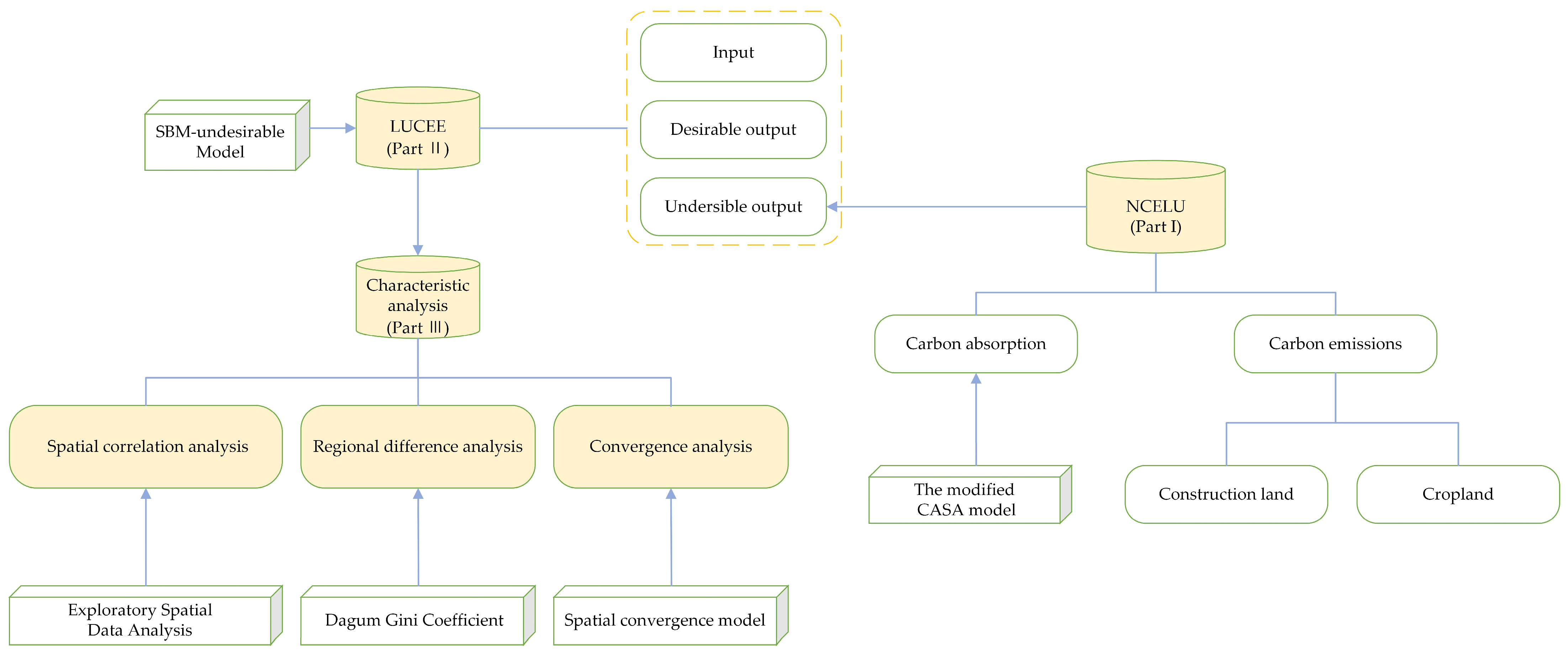
2.1. Research Framework

This study focuses on three parts (Figure 1): estimation of NCELU, measurement of LUCEE, and characteristic analysis of LUCEE. First, this study collects multi-source data from 98 cities in the PPRD from 2006 to 2020 and estimates the NCELU. Second, the NCELU is included as an undesirable output in the index system to measure the LUCEE using the SBM-undesirable model. Then, on the basis of the measurement of LUCEE, the characteristic analysis of LUCEE is conducted. In this study, ESDA, the Dagum Gini coefficient, and spatial convergence model are used to analyze the spatial correlation, regional differences, and convergence of LUCEE, respectively. Finally, policy recommendations are given based on the findings.

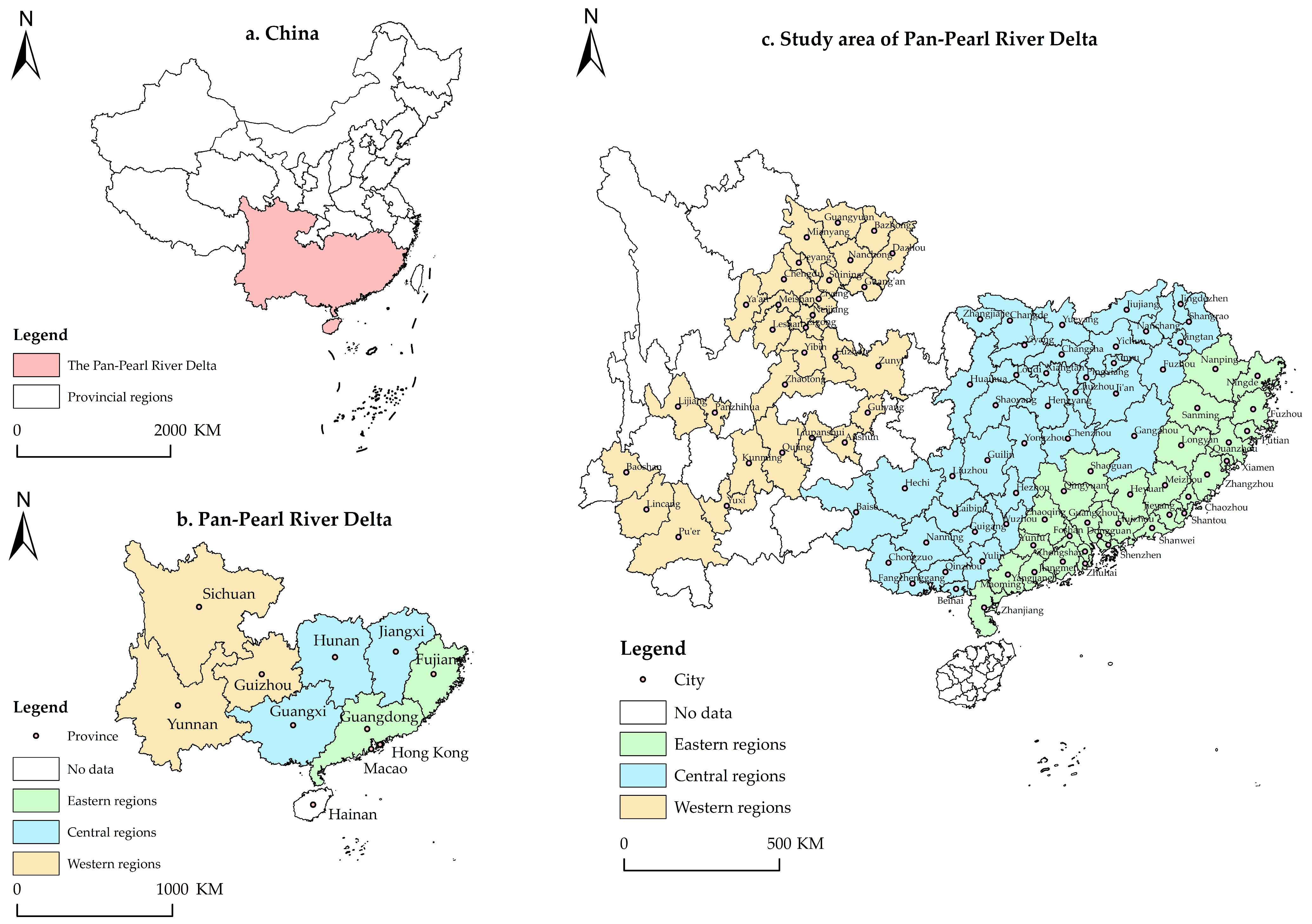
2.2. Study Area Overview

The PPRD can be traced back to 2003 when it was first proposed by Guangdong. The PPRD was officially launched in 2004 [32] and was designated as part of a national strategy in 2016 [33]. In addition, the PPRD has been successively included in the 13th and 14th Five-Year Plan [33]. The regional scope of the PPRD encompasses nine provinces and two special administrative regions, including Guangdong, Fujian, Jiangxi, Hunan, Guangxi, Hainan, Sichuan, Guizhou, Yunnan, Hong Kong, and Macao (Figure 2). The PPRD encompasses approximately one-fifth of the nation’s land area, one-third of its population, and produces over one-third of its total economic output [34]. Furthermore, the PPRD is a region in China that plays a crucial role in attaining carbon neutrality goals due to its significant economic development and carbon reduction potential. Considering the completeness of the administrative regions and the data availability, the study area of this work encompasses 98 cities above the prefecture level in eight provinces, excluding Hong Kong, Macao, Hainan Province, autonomous prefectures, and Tongren and Bijie in Guizhou Province [34].

The PPRD spans the eastern, central, and western regions of China, covering developed coastal areas and less developed inland regions. Significant disparities are observed in economic and social development as well as natural resource endowments, resulting in strong spatial heterogeneity within the region. This study divides the region into three subregions (eastern, central, and western regions) to comprehensively analyze the spatial pattern and regional disparities of the LUCEE, following the previous literature [35]. The eastern region encompasses 30 cities in Guangdong and Fujian provinces; the central region includes 38 cities in Hunan, Jiangxi, and Guangxi provinces; and the western region covers 30 cities in Sichuan, Guizhou, and Yunnan provinces.

2.3. Research Methods

2.3.1. Estimation Methods for LUCB

The estimation of LUCB is equivalent to the estimation of NCELU, which is based on the estimation of land use carbon emissions and sequestration. The NCELU is equal to the difference between carbon emissions and carbon absorption [36]. Therefore, this subsection can be divided into three parts, which are estimation methods for land use carbon emissions, land use carbon absorption, and the NCELU, in the order of the subtitles.

• Estimation Methods for Land Use Carbon Emissions

Land use carbon emissions mainly include carbon emissions from construction land and cropland [37]. The former are estimated based on the carbon emissions generated during the energy consumption process. Meanwhile, the latter are estimated based on the carbon emissions generated during agricultural production processes.

(1) Estimation of carbon emissions from construction land.

This work followed the approach of Qin and Gong [38]. First, the energy carbon emission statistics of each province from 2006 to 2020 were computed using the methodology offered by the Intergovernmental Panel on Climate Change (IPCC) [39]. ArcGIS 10.6.1 software was also utilized to compute the total NTL value of each province. Subsequently, a fitting was performed between the two sets of data to establish their relationship. Finally, the carbon emission statistics were allocated to the grid scale, and the energy carbon emissions at the city level were calculated by aggregating the NTL values of each city at the grid level.

Calculation of the provincial energy carbon emission statistics: this study selected nine major energy sources to calculate the provincial energy carbon emission statistics, based on the relevant literature [40,41]. The chosen energy sources included coal, coke, crude oil, gasoline, kerosene, diesel oil, fuel oil, natural gas, and electricity. The specific formula is as follows:

$$E_{it}=\frac{44}{12}\times {\displaystyle \sum _{j=1}^9\left(E_{ij}^t\times {\theta }_j\times K_j\right)}$$

(1)

where $E_{it}$ represents the provincial energy carbon emission statistics, measured in ten thousand tons; $E_{ij}^t$ represents the energy consumption; ${\theta }_j$ represents the standard coal conversion coefficient, sourced from the appendix of the “China Energy Statistical Yearbook”; $K_j$ represents the carbon emission coefficient, sourced from the carbon emission calculation guide issued by the IPCC; and $i$, $t$, and $j$ are the province, year, and energy type, respectively.

Inversion of the municipal energy carbon emissions: a linear model without an intercept term was used to guarantee the accuracy of the downscaling model inversion [42,43]. The linear model and fitting results are displayed in Equation (2) and

Table 1. Fitting results of municipal carbon emission inversion.

Province	K	R2
Fujian	0.0396	0.9701
Jiangxi	0.0599	0.9500
Hunan	0.0702	0.8969
Guangdong	0.0403	0.9880
Guangxi	0.0500	0.9837
Sichuan	0.0551	0.8941
Guizhou	0.0800	0.8464
Yunnan	0.0539	0.9792

, respectively. Table 1 illustrates that the R² of the linear regression equations of each province is higher than 0.8, indicating that the energy carbon emission statistics and the total NTL value in each province are well fitted and significantly correlated.

$$E_{it}=K\times D{N}_{it}$$

(2)

where $D{N}_{it}$ represents the total NTL value and $K$ represents the model coefficient.

Data accuracy correction: the municipal energy carbon emission estimates can be obtained by aggregating the NTL values at the grid level (Equation (2)). This paper applies correction techniques to the municipal energy carbon emission estimates by using provincial estimates and statistics of energy carbon emissions to enhance the data accuracy [38]. The final carbon emission from construction land is obtained through this correction process. The correction formula is as follows:

$$F{E}_{it}=T{E}_{nt}\times \left(N{C}_{it}/N{C}_{nt}\right)$$

(3)

where $F{E}_{it}$ represents the final corrected carbon emissions from urban construction land; $T{E}_{nt}$ represents the provincial energy carbon emission statistics; $N{C}_{it}$ represents the municipal energy carbon emission estimates; $N{C}_{nt}$ represents the provincial energy carbon emission estimates; and $i$, $n$ and $t$ are the city, province, and year, respectively.

(2) Estimation of the carbon emissions from cropland.

The carbon emissions mainly come from the inputs during the agricultural production process, such as the application of agricultural machinery, fertilizers, and carbon emissions, which result from the irrigation process. Carbon emissions from the application of fertilizers and carbon emissions from the irrigation process are equal to the amount of fertilizer used and the irrigated area multiplied by the corresponding carbon emission factors, respectively. Carbon emissions from the application of agricultural machinery are equal to the sum of the crop acreage and the total power of agricultural machinery multiplied by the corresponding coefficients [44]. The carbon emissions from cropland are the sum of the three. The formula is as follows:

$$C{E}_{it}=\left(S{P}_{it}\times a+P{P}_{it}\times b\right)+S{A}_{it}\times c+G{F}_{it}\times d$$

(4)

where $C{E}_{it}$ denotes the carbon emissions from cropland; $S{P}_{it}$ represents the crop acreage; $P{P}_{it}$ represents the total power of the agricultural machinery; $S{A}_{it}$ represents the irrigated area; $G{F}_{it}$ represents the amount of fertilizer used; and $a$, $b$, $c$, and $d$ represent their carbon emission factors, which are 16.47 kgC/hm², 0.18 kgC/kw, 266.48 kgC/hm², and 857.54 kgC/mg, respectively [45].

(3) Estimation of land use carbon emissions.

The value of the land use carbon emissions is the sum of the value of the carbon emissions from construction and land cropland, and the formula is as follows:

$$C_{it}^e=F{E}_{it}+C{E}_{it}$$

(5)

where $C_{it}^e$ represents the land use carbon emissions.

2.

Estimation Method for Land Use Carbon Absorption.

NPP can be utilized to measure the carbon stock and CO₂ absorbed by plants. This indicator is crucial for assessing terrestrial carbon cycling [16,46]. In this study, the estimation of land use carbon absorption is predicated on the calculation of NPP for every type of land use. With reference to relevant research [20], the formula is as follows:

$$C_{it}^s=\frac{NP{P}_{it}\times S_{it}}{45\%}\times 1.62$$

(6)

where $C_{it}^s$ represents the land use carbon absorption; $S_{it}$ represents the area of the region; and $NP{P}_{it}$ represents the NPP per unit area, which is estimated based on the modified CASA model, integrating meteorological and remote sensing image data simulations. The specific calculations of NPP can be found in reference [21], limited to space.

3.

Estimation Method for NCELU.

The NCELU is equal to the difference between carbon emissions and carbon absorption. The specific formula is as follows:

$$C_{it}=C_{it}^e-C_{it}^s$$

(7)

where $C_{it}$ represents the NCELU, $C_{it}$ < 0 indicates that the city is a carbon surplus region, and $C_{it}$ > 0 means that the city is a carbon deficit region.

2.3.2. SBM-Undesirable Model

LUCEE is assessed by using the SBM-undesirable model. Given that the model is sufficiently mature, this study does not further elaborate on its basic principles. The model expression is as follows:

$${\rho }^{*}=\min \frac{1-\frac{1}{m}{\displaystyle \sum _{i=1}^m\frac{S_i^{-}}{x_{i0}}}}{1+\frac{1}{a+b}({\displaystyle \sum _{r=1}^a\frac{S_r^e}{y_{r0}^e}+{\displaystyle \sum _{h=1}^b\frac{S_h^n}{y_{h0}^n})}}}$$

(8)

$$s.t.\left\{\begin{array}{l}{x}_0=X\lambda +S^{-}\\ y_0^e=Y^e\lambda -S^e\\ y_0^n=Y^n\lambda +S^n\\ S^{-}\ge 0,S^e\ge 0,S^n\ge 0,\lambda \ge 0\end{array}\right.$$

(9)

where ${\rho }^{*}$ represents the LUCEE of the cities, with a value between [0 and 1], and their efficiency is relatively effective only when ${\rho }^{*}$ = 1; and $\lambda$ represents the weight of inputs and outputs. The other letter symbols in the formula relate to inputs, desirable outputs, and undesirable outputs; $m$, $a$, and $b$ are their quantities; $x_{i0}$, $y_{r0}^e$, and $y_{h0}^n$ are their values; and $S^{-}$, $S^e$, and $S^n$ are their slack variables, respectively.

2.3.3. Exploratory Spatial Data Analysis (ESDA)

ESDA can be utilized to reflect the spatial correlation of a data index, including global and local spatial autocorrelation analyses [47]. This study investigates the global and local Moran’s index of the LUCEE to analyze the overall and local characteristics. The values of these indexes are between [−1 and 1], and the absolute magnitude is proportional to the strength of the spatial correlation. The formulas for calculating the global and local Moran’s index are shown in Equations (10) and (11), respectively.

$$I_G=\frac{{\displaystyle \sum _{i=1}^n{\displaystyle \sum _{j=1}^n{w}_{ij}(x_i-\overline{x})}}(x_j-\overline{x})}{{\sigma }^2{\displaystyle \sum _{i=1}^n{\displaystyle \sum _{j=1}^n{w}_{ij}}}}$$

(10)

$$I_L=\frac{(x_i-\overline{x})}{{\sigma }^2}{\displaystyle \sum _{j=1}^n{w}_{ij}(x_j-\overline{x})}$$

(11)

where $x_i$ and $x_j$ are the LUCEE of cities $i$ and $j$, respectively ($i$ ≠ $j$); $n$ is the sample size; $w_{ij}$ is the geographic distance spatial weight matrix; $\overline{x}$ is the mean of the LUCEE; and ${\sigma }^2=\frac{1}{n}{\displaystyle \sum _{i=1}^n{(x_i-\overline{x})}^2}$ represents the variance of the LUCEE.

2.3.4. Dagum Gini Coefficient Decomposition Method

This model proposed by Dagum [48] effectively addresses the problem of cross-overlap of subsamples compared to the traditional Gini coefficient and Theil index. The model expression is as follows:

$$G=\frac{{\displaystyle \sum _{j=1}^k{\displaystyle \sum _{h=1}^k{\displaystyle \sum _{i=1}^{n_j}{\displaystyle \sum _{r=1}^{n_h}\left|y_{ji}-y_{hr}\right|}}}}}{2n^2\overline{y}}$$

(12)

where $G$ denotes the overall Gini coefficient; $k$ is the quantity of districts in the study region; $n_j$ and $n_h$ are the quantities of cities in districts $j$ and $h$, respectively; $y_{ji}$ and $y_{hr}$ denote the LUCEE of city $i$ in district $j$ and city $r$ in district $h$, respectively; $n$ is the quantity of all cities; and $\overline{y}$ is the average value of the LUCEE across all cities.

Furthermore, $G$ can be decomposed into three components: intra-regional differences ($G_w$), inter-regional net differences ($G_{nb}$), and hypervariable density ($G_t$). The specific calculations of these components can be found in the relevant references [49,50].

2.3.5. Spatial Convergence Model

The convergence suggests that the disparities among different regions will diminish over time, ultimately reaching a steady-state level where regional development levels converge. β convergence is a commonly used convergence model, suggesting that areas with lower starting levels of development will catch up to areas with higher starting levels due to faster development rates, resulting in a gradual reduction in regional disparities. The two types of β convergence are as follows: absolute and conditional β convergence, with the distinction lying in whether it assumes similarities in economic, social, and natural factors among regions. The former makes this assumption, while the latter does not [51,52]. If the regional LUCEE has a significant spatial correlation, then the spatial convergence model that considers spatial factors is a better choice compared with traditional convergence models [53]. Spatial convergence models mainly include the spatial lag model (SLM) and spatial error model (SEM). Their expressions are shown in Equations (13) and (14), respectively [54].

$$\ln \frac{LUCE{E}_{i,t+T}}{LUCE{E}_{i,t}}=\alpha +\beta \ln \left(LUCE{E}_{i,t}\right)+\rho w_{ij}\ln \frac{LUCE{E}_{i,t+T}}{LUCE{E}_{i,t}}+{\theta }_k{X}_{i,t}+{\phi }_i+v_t+{\epsilon }_{i,t}$$

(13)

$$\ln \frac{LUCE{E}_{i,t+T}}{LUCE{E}_{i,t}}=\alpha +\beta \ln \left(LUCE{E}_{i,t}\right)+\lambda w_{ij}{\epsilon }_{i,t}+{\theta }_k{X}_{i,t}+{\phi }_i+v_t+{\mu }_{i,t}$$

(14)

where $\ln \left(LUCE{E}_{i,t+T}/LUCE{E}_{i,t}\right)$ is the natural logarithm of the LUCEE growth rate in region $i$ during the period from $t$ to $t+T$; $\alpha$ and $\beta$ are the parameters to be estimated; $\beta$ < 0 suggests that convergence exists; the speed of convergence $s=-\ln (1+\beta )/T$ can be calculated from $\beta$; $\rho$ and $\lambda$ are the spatial correlation coefficients that reflect the influence of neighboring regions on the value of attributes of the region; $w_{ij}$ is the spatial weighting matrix based on geographical distance; ${\phi }_i$ and $v_t$ are the individual and time fixed effects, respectively; ${\epsilon }_{i,t}$ and ${\mu }_{i,t}$ are the random error terms; $X_{i,t}$ denotes the control variables; and ${\theta }_k$ is the coefficient of the control variables. When ${\theta }_k$ = 0, the above model is an absolute convergence model, and when ${\theta }_k$ ≠ 0, the above model is a conditional convergence model.

Considering the actual circumstances of the PPRD, six control variables that may affect the LUCEE were selected in the conditional convergence analysis of this study. The variables are detailed in

Table 2. Control variables selection for conditional convergence.

Variable	Measurement	Selection Reasons
Economic development level (ECO)	Expressed as GDP per capita	Regions with more advanced economic development can allocate more production factors to improve the LUCEE. These regions typically experience severe ecological damage, which can also have adverse effects on the LUCEE.
Industrial structure (IND)	Expressed as the ratio of tertiary to secondary output	This variable profoundly influences the energy structure. Industries characterized by high energy consumption and significant polluting levels are notable contributors to carbon emissions. A well-optimized industrial structure can effectively reduce carbon emissions, thus enhancing the LUCEE.
Population density (POP)	Expressed as the ratio of the total population in each city at the end of the year to the area of the administrative district	Regions with a high population density typically generate agglomeration effects, resulting in improved efficiency in land and energy utilization, thereby enhancing the LUCEE. However, a significantly high population density can also elevate energy consumption and strain the ecological carrying capacity of the land, restraining the enhancement of the LUCEE.
Foreign investment level (FDI)	Expressed as the ratio of the actual utilized foreign investment amount, converted based on the annual exchange rate, to the GDP for each prefecture-level city	The introduction of high-quality foreign investment is beneficial for improving the technological level in the study area, reducing energy consumption, decreasing carbon emissions, and enhancing the LUCEE. However, the introduction of foreign investment with high pollution may have the opposite effect.
Technical innovation level (INN)	Expressed as the proportion of R&D expenditure to GDP	The advancement in technical level can improve the land use efficiency and energy utilization, promote green economic growth, and enhance the LUCEE to a certain extent. In comparison with other indicators, the R&D investment of a region more accurately reflects its technological innovation capability; thus, its direct influence on the LUCEE is more pronounced.
Land use intensity (LUI)	Calculated using the assignment method by assigning values to the different types of land use (refer to relevant references for details of the calculation [55])	Land use intensity reflects the extent of exploitation and utilization of various land types. Studies have shown a significant positive correlation between land use intensity enhancement and urban carbon emissions [56].Therefore, land use intensity may affect the LUCEE through its influence on carbon emissions.

.

2.4. Indicator System Construction and Data Sources

2.4.1. Indicator System Construction

This study selects labor, fixed asset, and technological input as input indicators and economic output and net carbon emission output of land use as desirable and undesirable outputs, respectively, based on reference [5]. Moreover, the total amount of each indicator is divided by the corresponding regional land area, taking into account the differences in land resource endowments in the production process across cities. The indicators are detailed in

Table 3. Indicator system of the LUCEE.

Index Type	Index Description	Index Meaning	Index Unit
	Labor input per unit of land area	(Urban end-of-year employed population in urban units + urban private and individual employed population)/regional land area	Person/hm2
Input indicators	Fixed asset input per unit of land area	Gross fixed asset formation/regional land area	104 yuan/hm2
	Technological input per unit of land area	R&D expenditure/regional land area	104 yuan/hm2
Desirable output	Economic output per unit of land area	Gross GDP/regional land area	104 yuan/hm2
Undesirable output	Net carbon emission output per unit of land area	NCELU/regional land area	t/hm2

.

2.4.2. Data Sources and Data Processing

The data used cover two types: socio-economic data and geographic information data. The data details for each research content are specified in

Table 4. The sources and processing of the data required for each research content.

Research Content	Data Sources	Data Processing
Estimation of carbon emissions from construction land	The NTL data are from the research finding of Wu et al. (https://doi.org/10.7910/DVN/GIYGJU, accessed on 23 September 2023) [57]. The energy consumption data are from the China Energy Statistics Yearbook.	ArcGIS software is utilized to perform zonal statistics on NTL data, obtaining the total NTL values for each province and city.
Estimation of carbon emissions from cropland	The agricultural data are from the provincial and municipal statistical yearbooks, rural statistical yearbooks, and statistical bulletin.	Individual missing data are completed by interpolation.
Estimation of land use carbon absorption	The relevant meteorological data are from the China Meteorological Data Service Center (https://data.cma.cn/, accessed on 12 October 2023). The NDVI data are from the China Tibetan Plateau Science Data Center (https://data.tpdc.ac.cn/zh-hans/data/10535b0b-8502-4465-bc53-78bcf24387b3, accessed on 15 October 2023) [58]. The land use data are from annual China land cover dataset (CLCD) (https://zenodo.org/record/8176941, accessed on 15 October 2023) [59].	The relevant meteorological data are interpolated to obtain the required meteorological raster data. The land use data are resampled to ensure spatial resolution consistency with other data, all at a resolution of 250 m. Meanwhile, the land types are reclassified into cropland, woodland, grassland, water area, construction land, and unused land by referring to the land use classification system of the Chinese Academy of Sciences.
Measurement of LUCEE and conditional convergence analysis	The statistical data for the input and output variables required for efficiency measurement and the control variables required for conditional convergence analysis are from the China Urban Statistical Yearbook, the China Science and Technology Statistical Yearbook, the National Statistics Bulletin on Scientific and Technological Expenditure Inputs, and the statistical yearbooks and bulletins of the provinces and municipalities. The land area data are from the CLCD dataset.	All indicators involving prices are deflated with 2006 as the base period to eliminate the influence of the price factor. Individual missing data are completed by interpolation.

.

3. Results

According to the basic framework of this study, this section shows the calculation results of the LUCB and LUCEE, as well as the analysis results of the characteristics of LUCEE. Section 3.1 presents the estimation results of the LUCB. In this part, we analyze the results of the LUCB from two aspects of temporal evolution and spatial pattern, and the causes of LUCB change are assessed through the land use transfer matrix. Similarly, we analyze the spatial and temporal pattern of the LUCEE in Section 3.2, and the reasons for the change in LUCEE are determined according to the input–output ratio. In Section 3.3, Section 3.4 and Section 3.5, we study the spatial correlation, regional difference, and convergence of the LUCEE. The results of Section 3.3 show the spatial correlation and aggregation of the LUCEE. The results of Section 3.4 show the regional differences in LUCEE and their sources. Section 3.5 shows the convergence results of LUCEE. If the LUCEE of the study area converges, then the regional difference will gradually shrink over time.

3.1. Analysis of LUCC and the Difference in LUCB

3.1.1. Analysis of LUCC

The land use transfer matrix can visualize the value and direction of change in the area of each land category at the beginning and end of a certain time period in a region, and reveal the spatial and temporal evolutions of the inter-conversion between different land types [60].

Table 5. Transfer matrix of land use in research area from 2006 to 2020.

2006 to 2020	Cropland	Woodland	Grassland	Water Area	Unused Land	Construction Land	Loss Area
Cropland	350,550.07	51,001.61	2430.73	2378.98	23.06	11,613.43	67,447.81
Woodland	52,145.84	808,547.30	655.60	82.70	1.74	1279.16	54,165.04
Grassland	4027.26	3214.99	9942.38	157.71	45.47	326.29	7771.72
Water area	3172.99	177.35	50.06	19,712.01	32.72	829.94	4263.06
Unused land	10.98	1.14	48.21	45.96	72.36	16.93	123.22
Construction land	69.96	1.04	0.61	532.7	0.40	21,385.63	604.71
Gain land	59,427.03	54,396.13	3185.21	3198.05	103.39	14,065.75	134,375.56
Variation	−8020.78	231.09	−4586.51	−1065.01	−19.83	13,461.04

reports the results of the land use transfer matrix for the PPRD during the study period, where gain land refers to the gross area transferred from other land types to that land type, loss area refers to the gross area transferred from that land type to other land types, and the difference between the two values is the amount of change in that land type during the period of 2006–2020.

During the study period, the area of carbon source land increased and the area of carbon sink land decreased, and the carbon source land gained a total of 8020.78 km² from the carbon sink land. Among the carbon source land, cropland and construction land decreased by 8020.78 km² and increased by 13,461.04 km², respectively. All the other areas of carbon sink land, except for woodland, which had a small increase, had a decrease of different degrees. With regard to the dynamic transfer of each category, cropland had the largest area transferred out, totaling 67,447.81 km². The area of cropland transferred to forest and cropland transferred to construction land expansion accounted for the largest proportion, accounting for 75.62% and 17.22% of the area transferred out of cropland, respectively. The largest transferred-in area was also cropland, which was 59,427.03 km², and woodland was its main source of transfer in, accounting for 87.75% of the transferred-in area of cropland. The main sources of land area transferred into construction land were cropland and woodland and were much larger than the area transferred out.

In summary, the overall trend in the research area indicates an increase in carbon source land area and a decrease in carbon sink land area. Additionally, construction land area witnessed the most significant increase, encroaching on cropland and woodland.

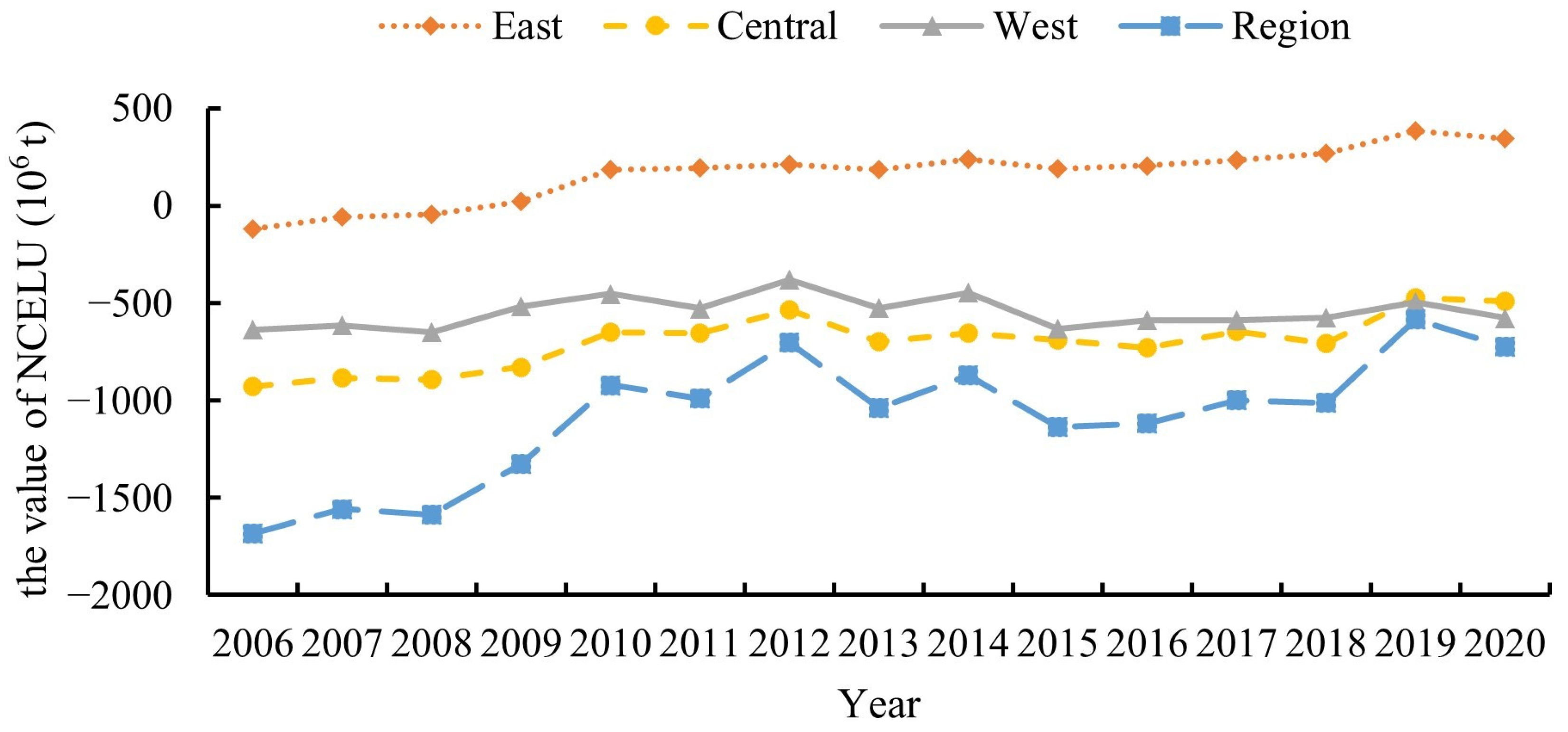
3.1.2. Analysis of the Spatial and Temporal Variations in LUCB

The NCELU for each city in the research area were estimated based on the estimation methods for LUCB. The results indicate that the research area remained a carbon surplus region throughout the study period (Figure 3). Additionally, the NCELU exhibited significant spatiotemporal differences.

(1) At the time scale, the NCELU was negative at the global level during the study period, but exhibited an increasing fluctuation (Figure 3). During the period of 2006–2020, the NCELU increased from −168.58 million tons to −724.65 million tons, an increase of 57.02%, which was related to the general increase in carbon source land and decrease in carbon sink land during the study period. At the regional level, the NCELU of each subregion also showed an upward trend. The eastern region experienced the most significant increase in NCELU, with −119.04 million tons in 2006 and 344.83 million tons in 2020, representing an increase of 389.68%. The smallest increase was observed in the western region, with −639.19 million tons in 2006 and −578.35 million tons in 2020, representing a 9.52% increase. The NCELU in the eastern region was the only region among the three with a carbon deficit, indicating significant pressure for carbon reduction. At the city level, 10 cities in the PPRD, including Nanning, Zhanjiang, and Xinyu, shifted from a carbon surplus to a carbon deficit from 2006 to 2020. Meanwhile, only one city, Liupanshui, realized the shift from a carbon deficit to a carbon surplus. The total quantity of cities with a carbon deficit increased from 22 to 31, suggesting ongoing pressure on the PPRD to achieve regional carbon neutrality.

(2) At the spatial scale, the NCELU basically exhibited the spatial distribution characteristic of “high in coastal and provincial cities and low in neighboring cities”, and this spatial distribution characteristic was gradually strengthened (Figure 4). A strong correlation potentially exists between the spatial distribution of NCELU and the degree of economic development of the cities. The low value areas with an NCELU of less than −50 million tons were mainly distributed in Yunnan Province and western Guangxi Province, which are relatively lagging behind in terms of economic development and have a high environmental carrying capacity. Meanwhile, the high value areas with an NCELU of more than 20 million tons were mainly distributed in the eastern coastal area, the Pearl River Delta urban agglomeration, and some provincial capital cities, where the population is concentrated, and the economy is well developed. During urbanization and industrialization processes, these cities occupied part of the ecological land, such as woodland and cropland, and consumed a substantial amount of “high carbon” energy to achieve rapid economic development, inducing a weakening of the carbon absorption capacity of the land and an increase in carbon emissions, which caused a severe carbon deficit.

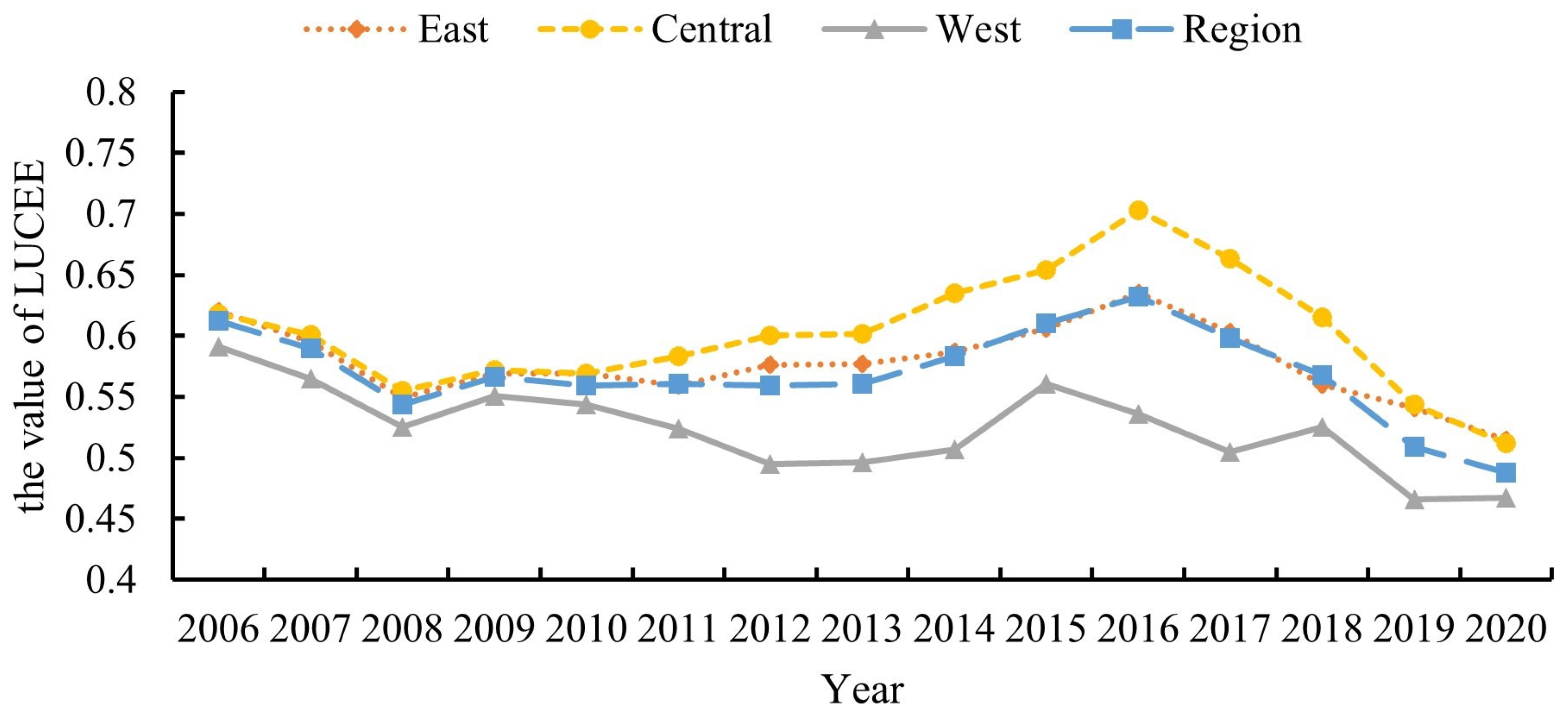
3.2. Spatiotemporal Pattern Analysis of LUCEE

The results show that the overall LUCEE from 2006 to 2020 is not high, and still has a large room for improvement (Figure 5). In addition, the LUCEE in the PPRD also exhibited evident spatiotemporal heterogeneity characteristics.

(1) At the time scale, the LUCEE from 2006 to 2020 shows a three-phase fluctuating downward trend of “decrease–rise–decrease” (Figure 5). The LUCEE first decreased from 0.612 in 2006 to 0.544 in 2008, then gradually increased to 0.632 in 2016, and finally decreased to 0.488 in 2020, with an annual decline rate of 1.60%.

The reason why the LUCEE went from a decline to an increase in 2008–2016 may be that, in terms of inputs and desirable output, in response to the economic shocks caused by the global financial crisis in 2008, the Chinese government chose to promote rapid economic growth through high investment, mainly in infrastructure and construction. During this period, the study area experienced a large increase in desirable output while expanding the scale of input factors. In terms of undesirable output, the study area, as a carbon surplus region, has a strong carbon absorption capacity and can better mitigate the negative influence of land development and “high carbon” energy use. Desirable output has a greater influence on LUCEE than undesirable output, and the input–output ratio is good.

Meanwhile, the reason why the LUCEE went from an increase to a decline in 2016–2020 may be that, in terms of inputs and desirable output, the study area entered a stage of pursuing high-quality development in this period, with a slowdown in GDP growth despite further expansion of input factors. In terms of undesirable output, the study area has significantly relied on a “high carbon” development model in the process of urbanization and industrialization. Continuous high-intensity development of construction land has occupied a substantial portion of carbon sink land, inducing the gradual weakening of the carbon absorption capacity of the land in the region, and the scale of NCELU has been expanding. The undesirable output has a greater influence on LUCEE compared with the desirable output, and the input–output ratio deteriorates.

The evolution of LUCEE in the three subregions follows a similar trend to that of the entire region, with the efficiency levels being in order from highest to lowest in the central, eastern, and western regions. Fewer cities exhibited an increasing LUCEE than those with a decreasing LUCEE during the period of 2006–2020. A total of 22 cities, including Pu’er, Ya’an, and Beihai, had a rising LUCEE, while the other 76 cities had a declining LUCEE. Therefore, in the future, local governments should formulate policies according to local conditions and balance the relationship between development and emission reduction to optimize the input–output ratio and improve the LUCEE.

(2) At the spatial scale, the LUCEE shows a spatial distribution characterized by “high in the north and south, low in the middle” (Figure 6). Cities with high efficiency are relatively small in size and dispersed, sporadically scattered on the northern and southern sides of the PPRD. These areas typically have characteristics of economic development or good ecological conditions. Cities with low efficiency are mainly concentrated in the southern parts of Hunan and Jiangxi provinces and the western parts of Yunnan Province, which are located in the middle of the PPRD. These areas are relatively economically underdeveloped, but they have become demonstration areas for undertaking industrial transfers and “pollution paradises” for “high-carbon” industries due to their significant advantages in production factors, such as land, labor, and energy.

In 2020, a total of 14 cities reached the efficiency frontier, of which six were carbon deficit cities, including Guangzhou, Shenzhen, Foshan, Dongguan, Beihai, and Deyang. These cities achieved the efficiency frontier with a relatively high desirable output. The remaining eight cities were carbon surplus cities, namely, Changde, Maoming, Zhaoqing, Yunfu, Yulin, Guang’an, Ya’an, and Pu’er. These cities typically have good ecological conditions, relatively low land development intensity, and fewer “high-carbon” industries, achieving the efficiency frontier with a lower undesirable output.

3.3. Spatial Correlation Analysis of LUCEE

3.3.1. Global Spatial Autocorrelation Analysis of LUCEE

Table 6. Global Moran’s I of the LUCEE from 2006 to 2020.

Year	G-Moran’s I	Z-Value	p-Value	Year	G-Moran’s I	Z-Value	p-Value
2006	0.1363	2.0176	0.0266	2014	0.3807	5.3581	0.0000
2007	0.0944	1.4440	0.0788	2015	0.3517	4.9608	0.0000
2008	0.1275	1.9003	0.0353	2016	0.4332	6.0651	0.0000
2009	0.1285	1.9115	0.0332	2017	0.5088	7.1441	0.0000
2010	0.1704	2.4811	0.0102	2018	0.2829	4.0193	0.0001
2011	0.1968	2.8417	0.0043	2019	0.3054	4.3633	0.0002
2012	0.2756	3.9268	0.0003	2020	0.2715	3.8997	0.0004
2013	0.3713	5.2333	0.0000

demonstrates that the global Moran’s I values of the LUCEE are all positive, and only one year, 2007, is insignificant. The coefficients and significance show an increasing trend, indicating a significant positive spatial correlation in LUCEE (i.e., an obvious spatial agglomeration characteristic).

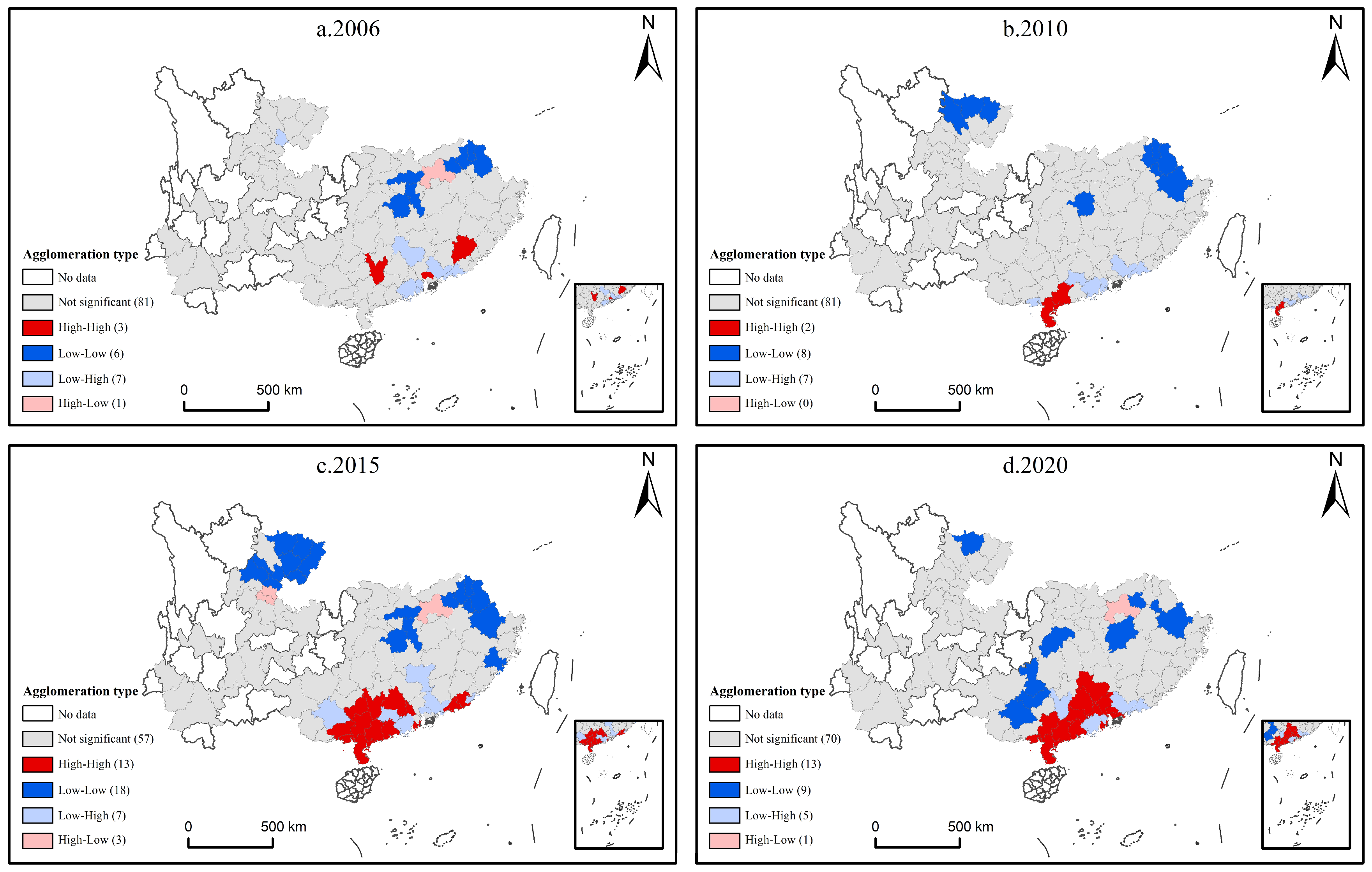
3.3.2. Local Spatial Autocorrelation Analysis of the LUCEE

LISA cluster maps for 2006, 2010, 2015, and 2020 were generated based on the results of the local Moran’s I values at the 10% significance level to further specifically analyze the spatial agglomeration characteristics of CLUEE (Figure 7). The results indicate that the spatial clustering degree of the LUCEE in the cities of the PPRD showed an increasing trend from 2006 to 2020. The LUCEE of cities exhibited four types of clustering characteristics: high–high, low–low, low–high, and high–low, with high–high and low–low clustering predominating.

During the period of 2006–2020, the agglomeration of the high–high and low–low ag-glomeration regions expanded, which added 10 and 3 cities, respectively. The high–high clustering areas underwent a development process from dispersion to aggregation. The high–high clustering areas were discretely distributed in Meizhou and Dongguan in Guangdong and Wuzhou in Guangxi in 2006. By 2020, it had formed a clustered distribution that included most of the cities in Guangdong and a few cities in the eastern part of Guangxi. The high–high clustering areas transformed from a small, scattered distribution to a large, concentrated distribution, indicating a significant positive spatial spillover effect among cities in these areas over time. The intensive flow of production factors between the neighboring cities drove the LUCEE level of the surrounding, less-developed cities. The low–low clustering areas transformed from a dual-core agglomeration distribution to a discrete distribution of southward migration. This phenomenon suggests that the negative spatial spillover effect of the LUCEE in the PPRD did not improve during the study period. In the future, these areas should limit land development intensity and strengthen regional ecological protection and restoration, thereby reducing undesirable output and improving the LUCEE.

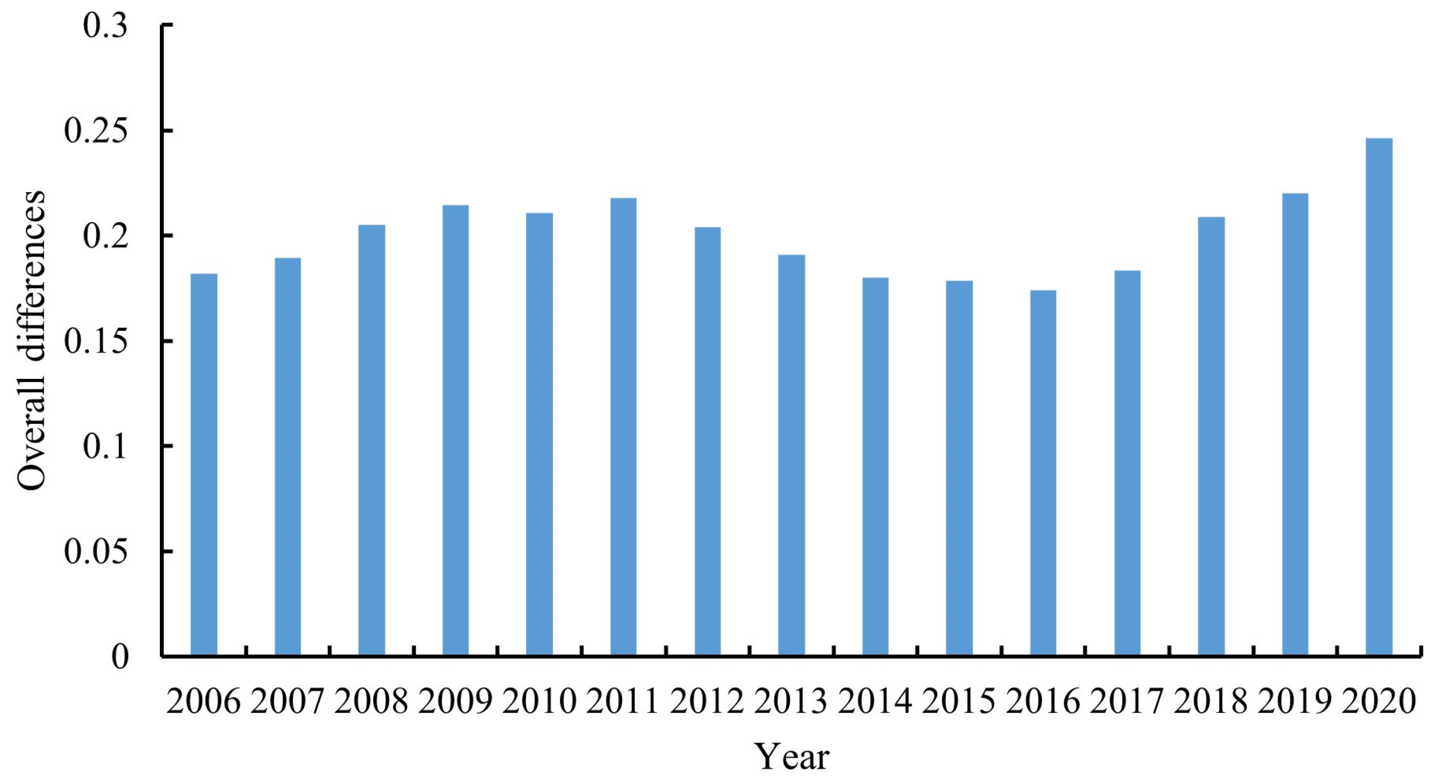
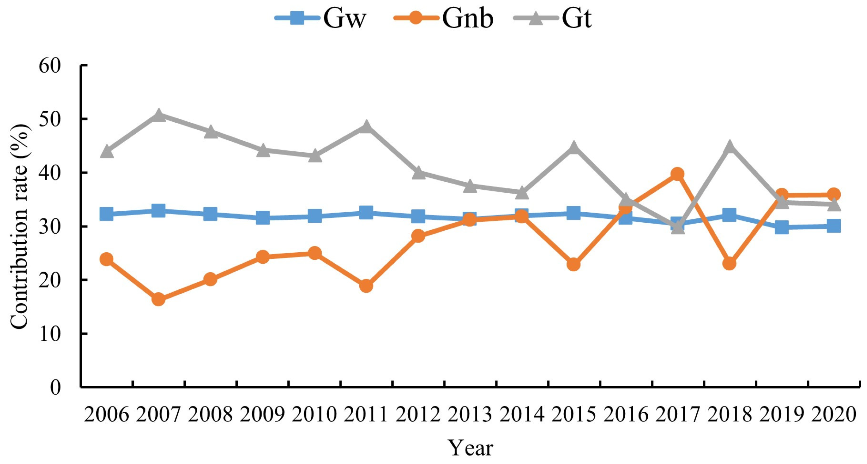
3.4. Regional Difference Analysis of LUCEE

Table 7. Gini coefficient decomposition results of LUCEE.

Year	Overall	Intra-Regional Differences			Inter-Regional Differences			Contribution Rate (%)
		East	Central	West	East– Central	East– West	Central– West	${\mathit{G}}_{\mathit{w}}$	${\mathit{G}}_{\mathit{n}\mathit{b}}$	${\mathit{G}}_{\mathit{t}}$
2006	0.1819	0.1665	0.1819	0.1748	0.1923	0.1826	0.1806	32.20	23.82	43.99
2007	0.1893	0.1868	0.1866	0.1798	0.1968	0.1933	0.1844	32.85	16.34	50.81
2008	0.2050	0.2083	0.1795	0.2101	0.2112	0.2195	0.1978	32.22	20.11	47.68
2009	0.2143	0.2047	0.1767	0.2365	0.2178	0.2314	0.2139	31.55	24.27	44.18
2010	0.2108	0.2049	0.1844	0.2189	0.2197	0.2229	0.2060	31.83	24.99	43.19
2011	0.2178	0.2165	0.2058	0.2112	0.2248	0.2301	0.2104	32.50	18.87	48.63
2012	0.2039	0.1974	0.1849	0.1986	0.2064	0.2293	0.1969	31.76	28.17	40.07
2013	0.1909	0.1741	0.1685	0.1982	0.1897	0.2188	0.1882	31.33	31.14	37.53
2014	0.1799	0.1672	0.1856	0.1461	0.1874	0.1920	0.1759	31.94	31.77	36.29
2015	0.1785	0.1670	0.1706	0.1795	0.1789	0.1910	0.1776	32.43	22.86	44.71
2016	0.1739	0.1723	0.1758	0.1214	0.1802	0.1917	0.1703	31.51	33.45	35.04
2017	0.1833	0.1740	0.1903	0.1088	0.2038	0.2060	0.1661	30.48	39.70	29.82
2018	0.2089	0.2050	0.2083	0.1780	0.2256	0.2185	0.1962	32.08	22.99	44.93
2019	0.2199	0.1987	0.1919	0.1987	0.2530	0.2421	0.1973	29.75	35.76	34.49
2020	0.2461	0.2131	0.2133	0.2457	0.2757	0.2593	0.2367	30.01	35.88	34.11
average value	0.2003	0.1904	0.1869	0.1871	0.2109	0.2152	0.1932	31.63	27.34	41.03

presents the Gini coefficient decomposition results of the LUCEE in the PPRD from 2006 to 2020. In general, the overall differences, intra-regional differences, and inter-regional differences of LUCEE expanded to varying degrees during the study period. $G_t$ is the main source of regional differences.

In terms of overall differences (Figure 8), the overall Gini coefficient of the LUCEE in the study period fluctuates between 0.1819 and 0.2461, with an annual growth rate of 2.18% and a mean of 0.2003. With regard to the evolution trend, the overall Gini coefficient shows a three-phase fluctuating upward trend characterized by “rise–fall–rise”, with periods of increase observed from 2006 to 2011 and from 2016 to 2020, and a period of decrease from 2011 to 2016. In most years, the trend remains upward, indicating a significant imbalance among the LUCEE of cities in the PPRD, with the level of imbalance continuously deepening.

In terms of intra-regional differences (Figure 9), the intra-regional differences in the eastern, central, and western regions all fluctuated upward. The eastern and central regions experienced smaller changes, with annual growth rates of 1.78% and 1.14%, respectively. Meanwhile, the western region experienced larger changes, with an annual growth rate of 2.46%. Overall, the intra-regional differences in descending order were in the eastern, western, and central regions, with mean Gini coefficients of 0.1904, 0.1871, and 0.1869, respectively. Notably, the intra-regional differences in the western region in 2020 were significantly larger than those in other regions, and imbalances in the western region need to be emphasized.

In terms of inter-regional differences (Figure 10), the differences between the eastern and other regions were consistently the largest of the inter-regional differences. Overall, the inter-regional differences rank in a descending order as east–west regions, east–central regions, and central–west regions. The mean Gini coefficients are 0.2152, 0.2109, and 0.1932, respectively. Regarding the evolution trend, the Gini coefficients between regions exhibit a similar fluctuating upward trend to the overall Gini coefficient, showing a “rise–fall–rise” pattern. The east–central and east–west regions have similar periods of rise and fall to the overall Gini coefficient, while the central–west region has the longest period of decline. The greatest fluctuation in Gini coefficients between regions is observed during the second upward period, indicating the most pronounced trend of differentiation.

In terms of the contribution rate (Figure 11), in most years, the contribution of $G_t$ to the overall differences was greater than those of $G_w$ and $G_{nb}$, indicating that $G_t$ constituted the primary source of the overall differences in the PPRD. This finding suggests that in most years, a clear cross-overlap effect of LUCEE exists, where the expansion of individual urban differences results in efficiency differentiation within regions. High LUCEE areas may also contain low LUCEE cities, and vice versa. The interaction between inter-regional and intra-regional differences has a significant influence on the overall differences in the LUCEE. Notably, $G_{nb}$ may gradually replace $G_t$ as the main source of spatial imbalance in LUCEE as the contribution rate of $G_t$ continues to decline and the contribution rate of $G_{nb}$ continues to rise.

3.5. Convergence Analysis of LUCEE

3.5.1. Convergence Model Selection

Selecting an appropriate convergence model is a prerequisite for examining the convergence of the LUCEE. According to the results of ESDA, a spatial econometric model that includes spatial effects needs to be selected for the convergence analysis. According to the judgment rule proposed by Anselin [61], the OLS regression is performed first to obtain the residuals, and then the Lagrange multiplier (LM) test and the Robust-LM test are performed, and the selection of SLM and SEM is determined by the outcomes of the test.

Table 8. Spatial correlation test of LUCEE.

Test Parameters	Absolute β Convergence		Conditional β Convergence
	T-Statistic	Prob.	T-Statistic	Prob.
Hausman	324.100	0.000	319.270	0.000
LM-lag	228.051	0.000	142.967	0.000
RLM-lag	1.560	0.212	1.848	0.174
LM-error	249.246	0.000	176.101	0.000
RLM-error	22.755	0.000	34.982	0.000

shows that LM-lag, LM-error and RLM-error passed the 1% significance level test for absolute and conditional convergence, while none of the RLM-lag passed the significance level test and the values of the T-statistic of RLM-error were greater than that of RLM-lag, so SEM was eventually chosen as the convergence model. Additionally, the Hausmann statistics all passed the 1% significance level test, suggesting that absolute and conditional convergence should be based on the fixed effects model. Considering the short-balanced panel data used in this study, each sample has its own individual variability and time-varying variability. Some omitted variable issues do not vary over time but differ across individuals, and vice versa [54]. Therefore, the SEM with spatiotemporal double fixed effects was constructed for the convergence analysis of the LUCEE.

3.5.2. Absolute Convergence Analysis of LUCEE

Table 9. Results of absolute and conditional β spatial convergence analysis.

Variable	Absolute β Spatial Convergence				Conditional β Spatial Convergence
	Region	East	Central	West	Region	East	Central	West
β	−0.4143 ***	−0.2573 ***	−0.5069 ***	−0.3960 ***	−0.4149 ***	−0.2669 ***	−0.5136 ***	−0.4350 ***
	(0.0190)	(0.0294)	(0.0329)	(0.0338)	(0.0190)	(0.0290)	(0.0340)	(0.0351)
ECO					0.0124 *	−0.0078	0.0903 **	0.0956
					(0.0075)	(0.0095)	(0.0492)	(0.0691)
IND					0.0772 ***	0.1586 ***	0.0535	0.0203
					(0.0231)	(0.0322)	(0.0384)	(0.0510)
POP					0.0727	−0.8132 **	0.9788	0.1965 *
					(0.0943)	(0.3376)	(4.6180)	(0.1163)
FDI					−0.7916 *	0.3726	−4.4761 ***	1.0011
					(0.4418)	(0.5274)	(1.0215)	(0.8459)
INN					−0.0212 *	0.0074	−0.0027	−0.0232
					(0.0111)	(0.0224)	(0.0195)	(0.0173)
LUI					−0.5965	0.7363	0.6437	−15.1327 ***
					(0.9287)	(0.8509)	(2.2464)	(3.7630)
λ	0.3331 ***	−0.1052	−0.0449	0.0926	0.3308 ***	−0.2290	−0.1767	0.1296
	(0.1213)	(0.1919)	(0.1659)	(0.1672)	(0.1228)	(0.2145)	(0.1846)	(0.1666)
s	0.0382	0.0212	0.0505	0.0360	0.0383	0.0222	0.0515	0.0408
R2	0.2645	0.1706	0.3262	0.2445	0.2790	0.2282	0.3417	0.2813

Notes: *, ** and *** Denote statistical significance at the 10%, 5%, and 1% levels, respectively. The standard errors are in parentheses.

reports the convergence results of the LUCEE for the entire region and three subregions. The results of the absolute convergence indicate the following: First, absolute β convergence can be observed in the LUCEE for the entire region and three subregions. The absolute convergence coefficients β in the models are negative and significant at the 1% level, indicating that without considering a range of economic, social, and natural factors affecting LUCEE, the LUCEE in the study region and its respective subregions will converge over time to their respective steady-state levels.

Second, different spatial effects can be observed in the LUCEE across the entire study area and its subregions. The spatial error term coefficient λ in LUCEE for the entire region is significant at the 1% level, suggesting that the residual terms of the cities have a significant diffusion effect on the LUCEE of the neighboring cities. Moreover, the improvement in LUCEE can accelerate the rate of convergence and reduces the overall differences. The λ coefficients of the LUCEE in the eastern and central regions are negative, and those of the LUCEE in the western region are positive, but none of them pass the significance level test, suggesting that the spatial effect of LUCEE convergence in the subregion has not yet manifested.

Third, differences exist in the convergence speed of the LUCEE across the entire study area and its subregions. The convergence speed in the entire region is 0.0382, and the regional convergence speeds are, from fastest to slowest, the central, western and eastern regions, with the convergence speeds of 0.0505, 0.0360, and 0.0212, respectively. The speed in the central region surpasses the speed in the entire region. In convergence theory, the assumption of absolute β convergence implies similarity in economic, social, and natural factors across regions, which may not hold true in reality. Therefore, a series of control variables need to be considered for further conditional β convergence analysis.

3.5.3. Conditional Convergence Analysis of LUCEE

The results of conditional convergence (Table 9) indicate the following: First, after adding the control variables of economic development level, industrial structure, population density, foreign investment level, technical innovation level and land use intensity, the R² of all the models significantly increases compared with that of the absolute β convergence analysis, indicating that the selection of the control variables has a certain rationality. Moreover, the conditional β convergence coefficients of LUCEE in the entire study area and in each subregion are significantly negative. This indicates that, after considering a series of economic and social factors, the LUCEE in the entire study area and each subregion still exhibit conditional convergence. The trend of the LUCEE in the entire study area and each subregion converging to their respective steady-state levels over time still exists. Second, the spatial effects of conditional convergence are no different from the absolute convergence analysis; thus, they are not further elaborated upon. Third, the speed of convergence of the regions is accelerated, but not significantly, compared with the absolute convergence results. The ordering of the speed of convergence of the regions is the same as that of the absolute convergence.

4. Discussion

4.1. Result Analysis

This study provides a research strategy for LUCEE that meets the current requirements for carbon neutrality based on existing research. This strategy offers higher accuracy and is suitable for long time series and large-scale samples compared with the carbon emission coefficient method. This strategy can be used for evaluating regional LUCEE and providing reference for the formulation of the subsequent carbon reduction policies.

(1) The results of the differences in LUCB show that the NCELU of the PPRD and its subregions show a fluctuating upward trend. The NCELU in the eastern part of the PPRD is significantly higher than that in the central and western parts. This observation is consistent with the spatial distribution characteristics of China’s NCELU, which is high in the east and low in the west [62]. The increase in land use carbon emissions is mainly due to the large expansion of construction land, which is consistent with the existing research results [9]. The areas of the PPRD with high carbon emission are mainly distributed in the eastern coastal areas, the Pearl River Delta urban agglomerations, and some provincial capitals. Wei et al. [63] found that the eastern coastal areas and the western provincial capitals are areas with high carbon emissions, which verified the conclusion.

(2) The measurement results of LUCEE show that the overall LUCEE is not high during the study period. Influenced by changes in GDP growth rate and land carbon absorption capacity, the LUCEE in the PPRD and its three subregions shows a fluctuating downward trend. The areas with a high LUCEE are mostly areas with better economic development, which is the same as in previous studies [64,65]. For example, Huang [64] found that the carbon emission efficiency of economically developed provinces in the PPRD is generally higher than that of economically underdeveloped provinces. However, Huang [64] ignored carbon absorption. The present study considered the carbon sink role of land and found that some cities reach the efficiency frontier due to good ecological environment. This finding suggests that economic development and increasing carbon absorption can effectively enhance the LUCEE.

(3) The characteristic analysis results of LUCEE show that LUCEE has a positive spatial correlation, which mainly shows high–high and low–low clustering characteristics. The overall difference, intra-regional difference, and inter-regional difference of LUCEE in the PPRD and its subregions show a fluctuating upward trend of “rise–fall–rise”, which is opposite to the trend of LUCEE. This finding suggests that the improvement in overall LUCEE may help narrow regional differences. Aimed at the problem of whether the regional difference of LUCEE in the PPRD will narrow, we used the spatial convergence model for analysis. The results show that the LUCEE in the PPRD and its subregions show absolute and conditional β convergence, which implies that the LUCEE will gradually tend to their respective stable levels over time. Thus, regional differences will gradually decrease

(4) The main advantage of this study is the improvement in the estimation accuracy of NCELU, which ensures the accuracy of LUCEE. Previous studies have mostly used the carbon emission coefficient method to calculate land use carbon emissions and carbon absorption. The calculation accuracy depends on the empirical coefficient of related research, while the unified empirical coefficients may be inapplicable to all study areas. Gui et al. [1] emphasized differences in the carbon emission factors of different cities and years, and the differences in the carbon emission factors of different types of cities are even greater. In addition, the carbon emission coefficient method may underestimate the regional carbon absorption, which in turn leads to an overestimation of the NCELU. This overestimation affects the accuracy of the LUCEE measurement. Zhang et al. [66] measured the NCELU of each province in China using the carbon emission coefficient method, and the results showed that the NCELU of Yunnan, Guizhou, Guangxi, and Sichuan are all positive. However, Wang et al. [67] emphasized that Yunnan, Guizhou, and Guangxi provinces are the largest carbon sinks in China, which account for about 31.5% of the terrestrial carbon sinks. The results of Chuai et al. [68] also showed a negative NCELU in Yunnan and Sichuan. This finding suggests that the study of Zhang et al. [66] overestimated the NCELU to some extent, which may affect the accuracy of subsequent efficiency studies. The NCELU measured in this work for the western region in the PPRD is negative, which is consistent with the actual situation. This study fully considered the energy consumption and vegetation carbon sequestration capacity of each city, which reflects the actual situation of the NCELU. This way ensures the accuracy of the LUCEE.

4.2. Policy Recommendations

(1) Given that the increase in NCELU in the PPRD basically comes from the expansion of construction land and the shrinkage of the area of carbon sink land, low-carbon spatial planning options and ecological restoration modes of national land oriented toward the target of carbon neutrality must be explored. First, land use control should be strengthened to optimize the land use structure. The proportion of carbon sink land should be increased to reduce carbon emissions by tightly regulating the expansion of the scale of construction land, deforestation, and other land development behaviors that increase carbon emissions. Second, natural ecosystem protection and restoration should be carried out to increase carbon storage. Starting from the spatial governance of the national territory, the red line for ecological protection should be delineated, and nature reserves should be set up to systematically promote ecological protection and restoration, thereby enhancing the carbon sequestration capacity of the land. Finally, a set of LUCB accounting processes applicable to regional realities must be compiled, and a dynamic and accurate basic data platform must be established for the LUCB. Regular monitoring of the carbon emissions and carbon absorption of major land use types will help in providing data support for policy intervention in the process of land use.

(2) Improving the overall level of LUCEE in the PPRD requires the joint efforts of all parties, who should formulate differentiated sustainable carbon reduction and development strategies based on their own actual situation. Cities that have reached the efficiency frontier need to continue to balance the relationship between economic development and carbon emission reduction to achieve high-quality and sustainable development. Other cities that have not reached the efficiency frontier need to make efforts to optimize the factor input–output ratio to improve their LUCEE until they reach the efficiency frontier. Carbon deficit cities that have not reached the efficiency frontier should make rational use of land resources and develop a green economy by expanding investment in fixed assets and technological inputs on the basis of ecosystem protection and restoration to improve the LUCEE. Meanwhile, carbon surplus cities that have not reached the efficiency frontier should optimize the allocation of factors by expanding the labor force and investing in fixed assets and technological inputs within the scope of ecological carrying capacity to achieve economic growth and improve the LUCEE.

(3) Although the regional differences in LUCEE in the PPRD are currently widening, the LUCEE of each region will finally converge to their respective steady-state levels over time, and the regional gap will gradually narrow. Therefore, all parties should enhance regional carbon reduction cooperation and promote the flow of factors between regions to narrow the efficiency gap between regions and facilitate the realization of the regional carbon neutrality target, in addition to further strengthening economic cooperation. For example, although the less-developed central and western regions undertake industrial transfer from the more developed eastern regions to develop their local economies, the more developed eastern regions should share advanced management concepts and technological achievements to prevent a decline in LUCEE in the less developed central and western regions due to an increase in the industrial land and energy consumption. Given the presence of spatial agglomeration and convergence in the LUCEE of cities in the PPRD, the spatial spillover effect can be performed by the cities with high LUCEE levels on the neighboring cities with low LUCEE levels. The catching-up effect can be performed by the cities with low LUCEE levels on the cities with high LUCEE levels to gradually narrow down the regional gap and promote the convergence of the LUCEE of the PPRD to a high value.

5. Conclusions

In this work, multi-source data such as geographic information data and socio-economic data were obtained, and NTL data and the modified CASA model were used to account for the LUCB, which was then employed as a measure of undesirable output. On this basis, the LUCEE levels of 98 cities in the PPRD for the period of 2006–2020 were measured by the SBM-undesirable model, and their spatiotemporal patterns were analyzed. Furthermore, ESDA, the Dagum Gini coefficient, and spatial convergence models were employed to reveal spatial correlations, regional differences, and spatial convergence.

The results show that the NCELU fluctuates upward from −168.584 million tons to −724.65 million tons. The regions with a high NCELU are mainly concentrated in the eastern region, coastal cities, and provincial capitals. The LUCEE fluctuates downward from 0.612 to 0.488. Areas with high LUCEE are generally characterized by developed economies or good ecological conditions. The LUCEE has a positive spatial correlation, and the spatial agglomeration effect is increasing, which mainly shows high–high and low–low clustering characteristics. The regional differences in LUCEE are increasing, with the overall difference rising from 0.1819 to 0.2461. Hypervariable density is the main source of regional differences. Absolute and conditional β convergence are present in the LUCEE of the PPRD and its subregions. Thus, the regional differences will decrease over time. The methodology and results of this study can serve as a reference for the PPRD to formulate regional differentiated carbon reduction strategies, eliminate regional differences in LUCEE, and achieve regional carbon neutrality.

Notably, this study has some limitations: (1) This study measures the NCELU and LUCEE based on multi-source data, which improves the precision to a certain extent, but suffers from the shortcomings of the difficulty in obtaining data, the cumbersome process of data processing, and the need to wait for data updates. This situation is also the reason why the research time point of this study stays at 2020. (2) Providing monthly data for NCELU and LUCEE would provide policymakers with more comprehensive information and more reliable decision support than annual data. However, this study is limited by the data and methods, which results in a failure to measure the monthly data of the NCELU and LUCEE. (3) The focus of this study on efficiency measurement and characteristic analysis, limited to space, failed to analyze driving mechanisms, which is the direction further study should take to deepen the research in the future.

References

1. Gui, D.; He, H.; Liu, C.; Han, S. Spatio-temporal dynamic evolution of carbon emissions from land use change in Guangdong Province, China, 2000–2020. Ecol. Indic. 2023, 156, 111131. [Google Scholar] [CrossRef]
2. Friedlingstein, P.; O’Sullivan, M.; Jones, M.W.; Andrew, R.M.; Bakker, D.C.E.; Hauck, J.; Landschützer, P.; Le Quéré, C.; Luijkx, I.T.; Peters, G.P.; et al. Global Carbon Budget 2023. Earth Syst. Sci. Data 2023, 15, 5301–5369. [Google Scholar] [CrossRef]
3. Pan, X.; Guo, S.; Xu, H.; Tian, M.; Pan, X.; Chu, J. China’s carbon intensity factor decomposition and carbon emission decoupling analysis. Energy 2022, 239, 122175. [Google Scholar] [CrossRef]
4. Hong, Y.; Yu, H.; Lu, Y.; Peng, L. Balancing low-carbon and eco-friendly development: Coordinated development strategy for land use carbon emission efficiency and land ecological security. Environ. Sci. Pollut. Res. 2024, 31, 9495–9511. [Google Scholar] [CrossRef] [PubMed]
5. Feng, W.; Zhao, R.; Xie, Z.; Ding, M.; Xiao, L.; Sun, J.; Yang, Q.; Liu, T.; You, Z. Land Use Carbon Emission Efficiency and Its Spatial-temporal Pattern under Carbon Neutral Target: A Case Study of 72 Cities in the Yellow River Basin. China Land Sci. 2023, 37, 102–113. [Google Scholar]
6. Wang, Y.; Chai, J.; Zhang, H.; Yang, B. Evaluating construction land use efficiency under carbon emission constraints: A comparative study of China and the USA. Environ. Sci. Pollut. Res. 2022, 29, 49998–50009. [Google Scholar] [CrossRef] [PubMed]
7. Dong, F.; Zhu, J.; Li, Y.; Chen, Y.; Gao, Y.; Hu, M.; Qin, C.; Sun, J. How green technology innovation affects carbon emission efficiency: Evidence from developed countries proposing carbon neutrality targets. Environ. Sci. Pollut. Res. 2022, 29, 35780–35799. [Google Scholar] [CrossRef]
8. Wang, T.; Li, H. Assessing the spatial spillover effects and influencing factors of carbon emission efficiency: A case of three provinces in the middle reaches of the Yangtze River, China. Environ. Sci. Pollut. Res. 2023, 30, 119050–119068. [Google Scholar] [CrossRef] [PubMed]
9. Meng, Q.; Zheng, Y.; Liu, Q.; Li, B.; Wei, H. Analysis of Spatiotemporal Variation and Influencing Factors of Land-Use Carbon Emissions in Nine Provinces of the Yellow River Basin Based on the LMDI Model. Land 2023, 12, 437. [Google Scholar] [CrossRef]
10. Lu, X.; Zhang, Y.; Li, J.; Duan, K. Measuring the urban land use efficiency of three urban agglomerations in China under carbon emissions. Environ. Sci. Pollut. Res. 2022, 29, 36443–36474. [Google Scholar] [CrossRef]
11. Tone, K. A slacks-based measure of efficiency in data envelopment analysis. Eur. J. Oper. Res. 2001, 130, 498–509. [Google Scholar] [CrossRef]
12. Yang, B.; Chen, X.; Wang, Z.; Li, W.; Zhang, C.; Yao, X. Analyzing land use structure efficiency with carbon emissions: A case study in the Middle Reaches of the Yangtze River, China. J. Clean. Prod. 2020, 274, 123076. [Google Scholar] [CrossRef]
13. Meng, F.; Su, B.; Thomson, E.; Zhou, D.; Zhou, P. Measuring China’s regional energy and carbon emission efficiency with DEA models: A survey. Appl. Energy 2016, 183, 1–21. [Google Scholar] [CrossRef]
14. Kuang, B.; Lu, X.; Zhou, M.; Chen, D. Provincial cultivated land use efficiency in China: Empirical analysis based on the SBM-DEA model with carbon emissions considered. Technol. Forecast. Soc. Change 2020, 151, 119874. [Google Scholar] [CrossRef]
15. Lv, T.; Geng, C.; Zhang, X.; Li, Z.; Hu, H.; Fu, S. Impact of the intensive use of urban construction land on carbon emission efficiency: Evidence from the urban agglomeration in the middle reaches of the Yangtze River. Environ. Sci. Pollut. Res. 2023, 30, 113729–113746. [Google Scholar] [CrossRef]
16. Liu, X.; Wang, P.; Song, H.; Zeng, X. Determinants of net primary productivity: Low-carbon development from the perspective of carbon sequestration. Technol. Forecast. Soc. Change 2021, 172, 121006. [Google Scholar] [CrossRef]
17. Guan, X.; Shen, H.; Li, X.; Gan, W.; Zhang, L. A long-term and comprehensive assessment of the urbanization-induced impacts on vegetation net primary productivity. Sci. Total Environ. 2019, 669, 342–352. [Google Scholar] [CrossRef]
18. Potter, C.S.; Randerson, J.T.; Field, C.B.; Matson, P.A.; Vitousek, P.M.; Mooney, H.A.; Klooster, S.A. Terrestrial ecosystem production: A process model based on global satellite and surface data. Glob. Biogeochem. Cycles 1993, 7, 811–841. [Google Scholar] [CrossRef]
19. Ichii, K.; Matsui, Y.; Yamaguchi, Y.; Ogawa, K. Comparison of global net primary production trends obtained from satellite-based normalized difference vegetation index and carbon cycle model. Glob. Biogeochem. Cycles 2001, 15, 351–363. [Google Scholar] [CrossRef]
20. Wu, Y.; Wang, P.; Liu, X.; Chen, J.; Song, M. Analysis of regional carbon allocation and carbon trading based on net primary productivity in China. China Econ. Rev. 2020, 60, 101401. [Google Scholar] [CrossRef]
21. Zhu, W.; Pan, Y.; Zhang, J. Estimation of net primary productivity of Chinese terrestrial vegetation based on remote sensing. Chin. J. Plant Ecol. 2007, 31, 413. [Google Scholar]
22. Zhang, C.-Y.; Zhao, L.; Zhang, H.; Chen, M.-N.; Fang, R.-Y.; Yao, Y.; Zhang, Q.-P.; Wang, Q. Spatial-temporal characteristics of carbon emissions from land use change in Yellow River Delta region, China. Ecol. Indic. 2022, 136, 108623. [Google Scholar] [CrossRef]
23. Zhang, B.; Yin, J.; Jiang, H.; Chen, S.; Ding, Y.; Xia, R.; Wei, D.; Luo, X. Multi-source data assessment and multi-factor analysis of urban carbon emissions: A case study of the Pearl River Basin, China. Urban Clim. 2023, 51, 101653. [Google Scholar] [CrossRef]
24. Cui, X.; Lei, Y.; Zhang, F.; Zhang, X.; Wu, F. Mapping spatiotemporal variations of CO2 (carbon dioxide) emissions using nighttime light data in Guangdong Province. Phys. Chem. Earth Parts A/B/C 2019, 110, 89–98. [Google Scholar] [CrossRef]
25. Sun, Y.; Zheng, S.; Wu, Y.; Schlink, U.; Singh, R.P. Spatiotemporal Variations of City-Level Carbon Emissions in China during 2000–2017 Using Nighttime Light Data. Remote Sens. 2020, 12, 2916. [Google Scholar] [CrossRef]
26. Yang, Q.; Pu, L.; Jiang, C.; Gong, G.; Tan, H.; Wang, X.; He, G. Unveiling the spatial-temporal variation of urban land use efficiency of Yangtze River Economic Belt in China under carbon emission constraints. Front. Environ. Sci. 2023, 10, 1096087. [Google Scholar] [CrossRef]
27. Zhang, A.; Deng, R. Spatial-temporal evolution and influencing factors of net carbon sink efficiency in Chinese cities under the background of carbon neutrality. J. Clean. Prod. 2022, 365, 132547. [Google Scholar] [CrossRef]
28. Lu, X.; Kuang, B.; Li, J. Regional difference decomposition and policy implications of China’s urban land use efficiency under the environmental restriction. Habitat Int. 2018, 77, 32–39. [Google Scholar] [CrossRef]
29. Wang, Z.; Shao, H. Spatiotemporal differences in and influencing factors of urban carbon emission efficiency in China’s Yangtze River Economic Belt. Environ. Sci. Pollut. Res. 2023, 30, 121713–121733. [Google Scholar] [CrossRef]
30. Yang, H.; Wu, Q. Land use eco-efficiency and its convergence characteristics under the constraint of carbon emissions in China. Int. J. Environ. Res. Public Health 2019, 16, 3172. [Google Scholar] [CrossRef]
31. Fan, X.; Jiang, X. Regional differences and convergence of urban land green use efficiency in China under the constraints of carbon neutrality. Environ. Dev. Sustain. 2023, 1–27. [Google Scholar] [CrossRef]
32. Li, G.; Kuang, Y.; Huang, N.; Chang, X. Emergy synthesis and regional sustainability assessment: Case study of pan-pearl river delta in China. Sustainability 2014, 6, 5203–5230. [Google Scholar] [CrossRef]
33. Ye, Y.; Yan, S.; Zhu, S. Growth Trends and Heterogeneity of Total Factor Productivity in Nine Pan-PRD Provinces in China. Sustainability 2022, 14, 14154. [Google Scholar] [CrossRef]
34. Liu, T.; Li, Y. Green development of China’s Pan-Pearl River Delta mega-urban agglomeration. Sci. Rep. 2021, 11, 15717. [Google Scholar] [CrossRef] [PubMed]
35. Xi, X.; Wang, L. Factor Decomposition of Regional Economic Difference in Pan-Pearl River Delta. Geogr. Geo-Inf. Sci. 2008, 24, 51–56+65. [Google Scholar]
36. Yang, S.F.; Fu, W.J.; Hu, S.G.; Ran, P.L. Watershed carbon compensation based on land use change: Evidence from the Yangtze River Economic Belt. Habitat Int. 2022, 126, 102613. [Google Scholar] [CrossRef]
37. Lin, Q.; Zhang, L.; Qiu, B.; Zhao, Y.; Wei, C. Spatiotemporal Analysis of Land Use Patterns on Carbon Emissions in China. Land 2021, 10, 141. [Google Scholar] [CrossRef]
38. Qin, J.; Gong, N. The estimation of the carbon dioxide emission and driving factors in China based on machine learning methods. Sustain. Prod. Consum. 2022, 33, 218–229. [Google Scholar] [CrossRef]
39. 2006 IPCC Guidelines for National Greenhouse Gas Inventories. Available online: https://www.ipcc-nggip.iges.or.jp/public/2006gl/index.html (accessed on 25 September 2023).
40. Zhang, L.; Lei, J.; Wang, C.; Wang, F.; Geng, Z.; Zhou, X. Spatio-temporal variations and influencing factors of energy-related carbon emissions for Xinjiang cities in China based on time-series nighttime light data. J. Geogr. Sci. 2022, 32, 1886–1910. [Google Scholar] [CrossRef]
41. Wei, W.; Du, H.; Ma, L.; Liu, C.; Zhou, J. Spatiotemporal dynamics of CO2 emissions using nighttime light data: A comparative analysis between the Yellow and Yangtze River Basins in China. Environ. Dev. Sustain. 2022, 26, 1081–1102. [Google Scholar] [CrossRef]
42. Yang, Z.; Chen, Y.; Guo, G.; Zheng, Z.; Wu, Z. Using nighttime light data to identify the structure of polycentric cities and evaluate urban centers. Sci. Total Environ. 2021, 780, 146586. [Google Scholar] [CrossRef]
43. Chen, S.; Tan, Z.; Mu, S.; Wang, J.; Chen, Y.; He, X. Synergy level of pollution and carbon reduction in the Yangtze River Economic Belt: Spatial-temporal evolution characteristics and driving factors. Sustain. Cities Soc. 2023, 98, 104859. [Google Scholar] [CrossRef]
44. Chen, Z.; Liu, Y.; Lin, H. Decoupling Analysis of Land-Use Carbon Emissions and Economic Development in Guangdong Province. Ecol. Econ. 2018, 34, 26–32. [Google Scholar]
45. West, T.O.; Marland, G. A synthesis of carbon sequestration, carbon emissions, and net carbon flux in agriculture: Comparing tillage practices in the United States. Agric. Ecosyst. Environ. 2002, 91, 217–232. [Google Scholar] [CrossRef]
46. Li, X.; Xiong, S.; Li, Z.; Zhou, M.; Li, H. Variation of global fossil-energy carbon footprints based on regional net primary productivity and the gravity model. J. Clean. Prod. 2019, 213, 225–241. [Google Scholar] [CrossRef]
47. Anselin, L.; Sridharan, S.; Gholston, S. Using Exploratory Spatial Data Analysis to Leverage Social Indicator Databases: The Discovery of Interesting Patterns. Soc. Indic. Res. 2007, 82, 287–309. [Google Scholar] [CrossRef]
48. Dagum, C. A new approach to the decomposition of the Gini income inequality ratio. Empir. Econ. 1997, 4, 515–531. [Google Scholar] [CrossRef]
49. Zhang, L.; Ma, X.; Ock, Y.-S.; Qing, L. Research on Regional Differences and Influencing Factors of Chinese Industrial Green Technology Innovation Efficiency Based on Dagum Gini Coefficient Decomposition. Land 2022, 11, 122. [Google Scholar] [CrossRef]
50. Han, H.; Ding, T.; Nie, L.; Hao, Z. Agricultural eco-efficiency loss under technology heterogeneity given regional differences in China. J. Clean. Prod. 2020, 250, 119511. [Google Scholar] [CrossRef]
51. Liu, N.; Wang, Y. Urban Agglomeration Ecological Welfare Performance and Spatial Convergence Research in the Yellow River Basin. Land 2022, 11, 2073. [Google Scholar] [CrossRef]
52. Yu, Q.; Li, Y.; Zhu, Y.; Chen, B.; Wang, Q.; Huang, D.; Wen, C. Spatiotemporal divergence and convergence test of green total factor productivity of grain in China: Based on the dual perspective of carbon emissions and surface source pollution. Environ. Sci. Pollut. Res. 2023, 30, 80478–80495. [Google Scholar] [CrossRef] [PubMed]
53. Ge, K.; Zou, S.; Chen, D.; Lu, X.; Ke, S. Research on the Spatial Differences and Convergence Mechanism of Urban Land Use Efficiency under the Background of Regional Integration: A Case Study of the Yangtze River Economic Zone, China. Land 2021, 10, 1100. [Google Scholar] [CrossRef]
54. Liu, M.; Zhang, A.; Wen, G. Regional differences and spatial convergence in the ecological efficiency of cultivated land use in the main grain producing areas in the Yangtze Region. J. Nat. Resour. 2022, 37, 477–493. [Google Scholar] [CrossRef]
55. Meng, Q.; Liu, Q.; Li, B.; Zheng, Y.; Cai, E. Decoupling Relationship Between Land Use Intensity and Carbon Emissions in Henan Province During 2000—2020. Bull. Soil Water Conserv. 2023, 43, 421–429. [Google Scholar]
56. Ali, G.; Nitivattananon, V. Exercising multidisciplinary approach to assess interrelationship between energy use, carbon emission and land use change in a metropolitan city of Pakistan. Renew. Sustain. Energy Rev. 2012, 16, 775–786. [Google Scholar] [CrossRef]
57. Wu, Y.; Shi, K.; Chen, Z.; Liu, S.; Chang, Z. Developing Improved Time-Series DMSP-OLS-Like Data (1992–2019) in China by Integrating DMSP-OLS and SNPP-VIIRS. IEEE Trans. Geosci. Remote Sens. 2022, 60, 4407714. [Google Scholar] [CrossRef]
58. Gao, J.; Shi, Y.; Zhang, H.; Chen, X.; Zhang, W.; Shen, W.; Xiao, T.; Zhang, Y. China Regional 250 m Normalized Difference Vegetation Index Data Set (2000–2022); National Tibetan Plateau/Third Pole Environment Data Center: Tibet, China, 2023. [Google Scholar]
59. Yang, J.; Huang, X. The 30 m annual land cover dataset and its dynamics in China from 1990 to 2019. Earth Syst. Sci. Data 2021, 13, 3907–3925. [Google Scholar] [CrossRef]
60. Mallinis, G.; Koutsias, N.; Arianoutsou, M. Monitoring land use/land cover transformations from 1945 to 2007 in two peri-urban mountainous areas of Athens metropolitan area, Greece. Sci. Total Environ. 2014, 490, 262–278. [Google Scholar] [CrossRef] [PubMed]
61. Anselin, L. Spatial Econometrics: Methods and Models; Springer Science & Business Media: Berlin/Heidelberg, Germany, 1988; Volume 4. [Google Scholar]
62. Wu, B.; Zhang, Y.; Wang, Y.; Wu, S.; Wu, Y. Spatio-temporal variations of the land-use-related carbon budget in Southeast China: The evidence of Fujian province. Environ. Res. Commun. 2023, 5, 115015. [Google Scholar] [CrossRef]
63. Wei, W.; Hao, R.; Ma, L.; Xie, B.; Zhou, L.; Zhou, J. Characteristics of carbon budget based on energy carbon emissions and vegetation carbon absorption. Environ. Monit. Assess. 2024, 196, 134. [Google Scholar] [CrossRef]
64. Huang, X. Carbon Efficiency Of Provinces In Pan -Yangtze River Delta, Pan-Pearl River Delta, And Circum-Bohai Region. Energy Rev. 2018, 2, 16–18. [Google Scholar]
65. Wu, H.; Fang, S.; Zhang, C.; Hu, S.; Nan, D.; Yang, Y. Exploring the impact of urban form on urban land use efficiency under low-carbon emission constraints: A case study in China’s Yellow River Basin. J. Environ. Manag. 2022, 311, 114866. [Google Scholar] [CrossRef]
66. Zhang, P.; He, J.; Hong, X.; Zhang, W.; Qin, C.; Pang, B.; Li, Y.; Liu, Y. Carbon sources/sinks analysis of land use changes in China based on data envelopment analysis. J. Clean. Prod. 2018, 204, 702–711. [Google Scholar] [CrossRef]
67. Wang, J.; Feng, L.; Palmer, P.I.; Liu, Y.; Fang, S.; Bösch, H.; O’Dell, C.W.; Tang, X.; Yang, D.; Liu, L. Large Chinese land carbon sink estimated from atmospheric carbon dioxide data. Nature 2020, 586, 720–723. [Google Scholar] [CrossRef]
68. Chuai, X.; Xia, M.; Ye, X.; Zeng, Q.; Lu, J.; Zhang, F.; Miao, L.; Zhou, Y. Carbon neutrality check in spatial and the response to land use analysis in China. Environ. Impact Assess. Rev. 2022, 97, 106893. [Google Scholar] [CrossRef]
Figure 1. The overall framework of the study.
Land 13 00634 g001
Figure 2. Overview of the study area: figures (ac) are China, the PPRD, and the study area of the PPRD selected for this study, respectively.
Land 13 00634 g002
Figure 3. Trends in the evolution of the time series of NCELU in the PPRD.
Land 13 00634 g003
Figure 4. Spatial pattern of the NCELU in the PPRD.
Land 13 00634 g004
Figure 5. Trends in the evolution of the time series of LUCEE in the PPRD.
Land 13 00634 g005
Figure 6. Spatial pattern of the LUCEE in the PPRD.
Land 13 00634 g006
Figure 7. LISA cluster map of the LUCEE from 2006 to 2020.
Land 13 00634 g007
Figure 8. Overall differences in LUCEE from 2006 to 2020.
Land 13 00634 g008
Figure 9. Intra-regional differences in LUCEE from 2006 to 2020.
Land 13 00634 g009
Figure 10. Inter-regional differences in LUCEE from 2006 to 2020.
Land 13 00634 g010
Figure 11. Contribution rate in LUCEE from 2006 to 2020.
Land 13 00634 g011