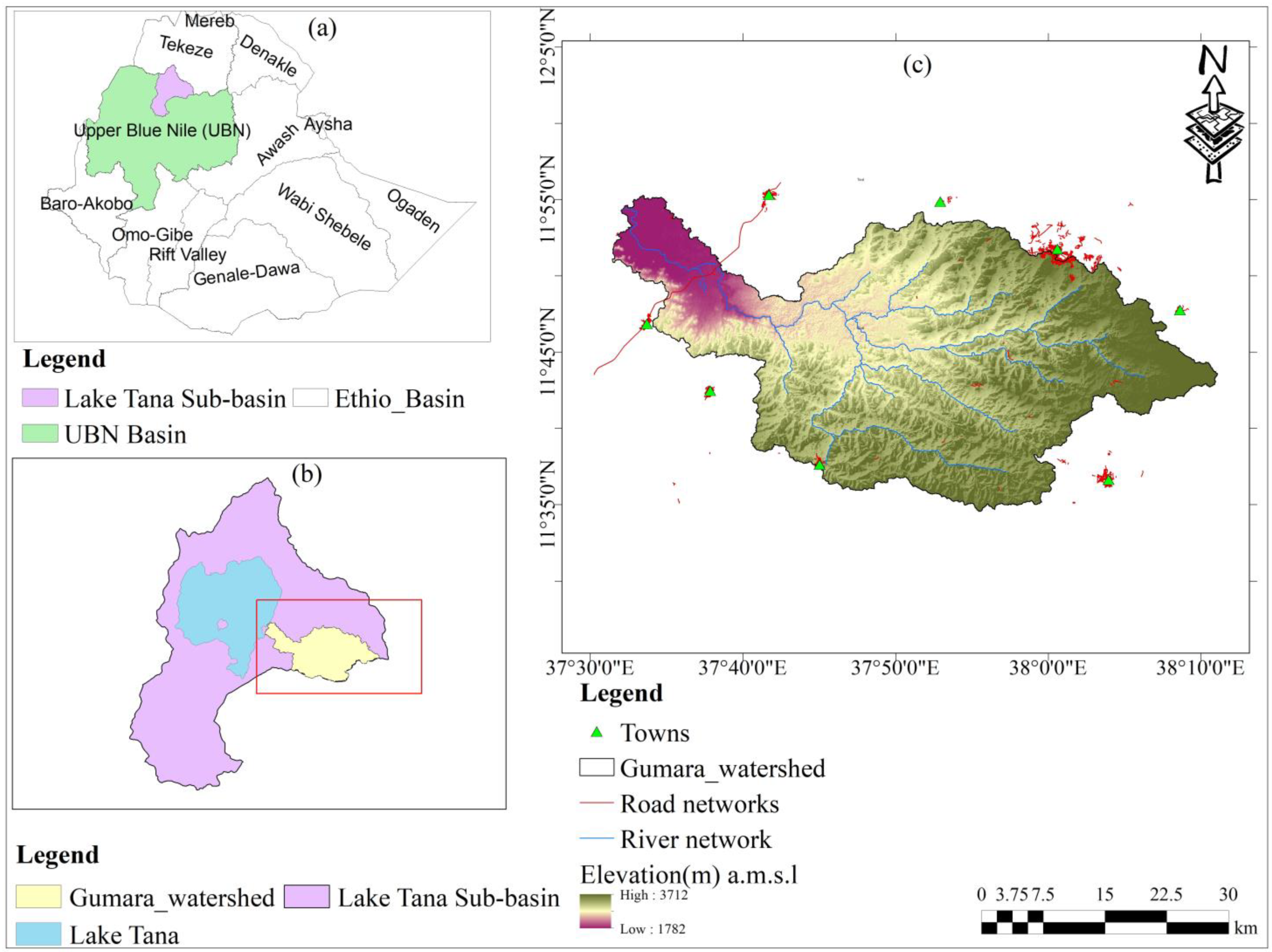
Article

Scenario-Based Land Use and Land Cover Change Detection and Prediction Using the Cellular Automata–Markov Model in the Gumara Watershed, Upper Blue Nile Basin, Ethiopia

1
Africa Center of Excellence for Water Management, Addis Ababa University, Addis Ababa P.O. Box 1176, Ethiopia
2
Department of Hydraulic and Water Resources Engineering, Dilla University, Dilla P.O. Box 419, Ethiopia
3
Department of Earth and Environment, Florida International University, Miami, FL 33199, USA
4
Department of Civil Engineering, Sustainable Energy Center of Excellence, Addis Ababa Science and Technology University, Addis Ababa P.O. Box 16417, Ethiopia
*
Authors to whom correspondence should be addressed.
Land 2024, 13(3), 396; https://doi.org/10.3390/land13030396
Submission received: 8 January 2024 / Revised: 1 March 2024 / Accepted: 18 March 2024 / Published: 20 March 2024
(This article belongs to the Special Issue Future Scenarios of Land Use and Land Cover Change)

Abstract

:
Land use and land cover (LULC) change detection and prediction studies are crucial for supporting sustainable watershed planning and management. Hence, this study aimed to detect historical LULC changes from 1985 to 2019 and predict future changes for 2035 (near future) and 2065 (far future) in the Gumara watershed, Upper Blue Nile (UBN) Basin, Ethiopia. LULC classification for the years 1985, 2000, 2010, and 2019 was performed using Landsat images along with vegetation indices and topographic factors. The random forest (RF) machine learning algorithm built into the cloud-based platform Google Earth Engine (GEE) was used for classification. The results of the classification accuracy assessment indicated perfect agreement between the classified maps and the validation dataset, with kappa coefficients (K) of 0.92, 0.94, 0.90, and 0.88 for the LULC maps of 1985, 2000, 2010, and 2019, respectively. Based on the classified maps, cultivated land and settlement increased from 58.60 to 83.08% and 0.06 to 0.18%, respectively, from 1985 to 2019 at the expense of decreasing forest, shrubland and grassland. Future LULC prediction was performed using the cellular automata–Markov (CA–Markov) model under (1) the business-as-usual (BAU) scenario, which is based on the current trend of socioeconomic development, and (2) the governance (GOV) scenario, which is based on the Green Legacy Initiative (GLI) program of Ethiopia. Under the BAU scenario, significant expansions of cultivated land and settlement were predicted from 83.08 to 89.01% and 0.18 to 0.83%, respectively, from 2019 to 2065. Conversely, under the GOV scenario, the increase in forest area was predicted to increase from 2.59% (2019) to 4.71% (2065). For this reason, this study recommends following the GOV scenario to prevent flooding and soil degradation in the Gumara watershed. Finally, the results of this study provide information for government policymakers, land use planners, and watershed managers to develop sustainable land use management plans and policies.

1. Introduction

Recently, land use and land cover (LULC) change detection and prediction have become popular research topics in the area of remote sensing; thus, these issues have attracted the attention of several researchers and land use planners [1,2]. This is due to the significant effect of LULC changes on altering the hydrological characteristics of basins and watersheds [3,4], climate change [5], and other environmental issues [6]. Globally, different LULC classes of basins and watersheds have undergone considerable changes from one category to another due to increasing anthropogenic activities such as deforestation, agricultural expansion, urbanization, mining, and other related activities [7,8,9]. For this reason, regularly updating LULC maps is an important task for capturing the dynamic nature of land use [10].
For spatiotemporal LULC mapping, remotely sensed multispectral images available at various spatiotemporal resolutions provide vital information. Some of these images include Moderate Resolution Imaging Spectroradiometer (MODIS), Pourl’Observation de la Terre (SPOT), Synthetic Aperture Radar (SAR), Landsat series, Sentinel-2 missions, and Rapid Eye Earth Imaging System (REIS) images [1]. From these images, the Landsat series has been used in a number of LULC mapping studies [5,11].
In LULC classification studies, the use of cloud-free composites of time-series images is more strongly recommended than the use of single images [10,12]. However, the traditional methods of searching, filtering, cloud masking, compositing, downloading, and classifying time series images require high computing power and a large volume of data storage. For this purpose, Google Earth Engine (GEE), which is a cloud-based platform, can solve the problems associated with big data processing [7,13]. This platform has recently been considered a powerful tool for processing and analyzing large volumes of remote sensing data. In the GEE environment, there are various supervised machine learning (SML) classification algorithms. Some of these include decision tree (DT), random forest (RF), naive Bayes (NB), minimum distance (MD), and classification and regression tree (CART) methods [6,14,15]. In this regard, several studies comparing SML classifiers have recommended the RF algorithm because it has the highest classification accuracy and the potential to handle high-dimensional data with a minimum number of parameters [16,17,18]. Moreover, the use of topographic factors and spectral indices can improve classification accuracy [19].
In addition to the LULC classification discussed above, LULC prediction is important for simulating future landscape conditions and determining the potential driving factors that cause land use change. According to the comprehensive review of [1], there are various temporal prediction models (for example, the Markov chain and system dynamics (SD)) and spatial prediction models (for example, cellular automata (CA) and conversion of land use and its effects (CLUE)) and hybrids of the two model categories. Recently, LULC prediction using hybrid models, such as the cellular automata–Markov (CA–Markov) model, has become an effective approach because it integrates both spatial and temporal simulation powers of the CA and Markov models. For this reason, a number of researchers have applied the CA–Markov model for predicting future LULC dynamics at the basin, watershed, and even city levels [20,21,22].
The prediction of future LULC dynamics based on historical trends is a critical issue [23]. However, the assumption of the continuity of the current land use trend is mostly susceptible to uncertainties due to the dynamic nature of land use change driver variables [24,25]. For this purpose, scenario-based LULC change analysis is mostly recommended as a tool to explore such uncertainties [26]. Recently, five shared socioeconomic pathways (from SSP1to SSP5) have been proposed for possible future socioeconomic development, climate change, and land use policies [27,28]. These SSP-based pathways provide information for research and policies related to land use and climate change to reduce the adverse impacts of rapid population growth, intensive agricultural cultivation, and greenhouse gas emissions [28]. Therefore, several scenario-based LULC change analysis studies have also been conducted at different spatiotemporal scales. For example, Wang, et al. [29] employed the CA–Markov model for simulating future LULC under environmental protection (EPS), crop protection (CP), and spontaneous (SP) scenarios in Tianjin city. The authors found a dramatic increase in built-up areas under the SP scenario relative to those under the EP and CP scenarios. Similarly, Gebresellase, et al. [30] simulated future LULC dynamics in the Upper Awash Basin of Ethiopia using the CA–Markov model for the years 2030 and 2060 under the BAU and governance (GOV) scenarios considering various spatial driving variables. The authors found a significant increase in cultivated land and settlement under the BAU scenario and an increase in forest area under the GOV scenario.
In Ethiopia, several studies have been conducted on historical LULC change detection at the basin and watershed scales [31,32,33]. These historical LULC change detection studies are vital for better understanding the interactions between human activities and their surroundings [34,35]. In addition to historical LULC change detection, information on future LULC change trends over a long period of time is also critical. As LULC change rapidly varies in Ethiopia due to human and natural factors [36], modelling and documenting future LULC dynamics is important for providing information for land use planners and policymakers to develop sustainable land use management plans [37]. However, in Ethiopia, less attention has been given to the prediction of future LULC dynamics, except for a few recent studies conducted in the Omo-Gibe River Basin [38], Upper Awash River Basin [30], Nashe watershed [21], Goang watershed [22], Majang Forest biosphere Reserve [2], and Addis Ababa and surrounding areas [39].
The Gumara watershed is a subwatershed of the Lake Tana subbasin in the Upper Blue Nile Basin (UBNB) of Ethiopia. Previous studies conducted in watersheds frequently used the maximum likelihood (ML) algorithm for LULC classification [40,41], which requires normally distributed data for classification [42]. However, less consideration has been given to robust machine learning classifiers such as the RF algorithm, which does not require the assumption that the data need to be normally distributed. The Gumara watershed was selected as the study area since it is highly prone to soil erosion in the uplands and flooding in the lowlands resulting from LULC change [36,43]. For these reasons, the present study aims (1) to map the historical LULC dynamics using the RF algorithm built into the GEE environment for the years 1985, 2000, 2010, and 2019; (2) to detect LULC changes in the historical period (1985–2019); and (3) to predict future LULC dynamics under the BAU and GOV for the years 2035 and 2065 using the CA–Markov model, which is available from the IDRISI Selva17.0 software package. In this regard, the BAU scenario is based on the current trends of socioeconomic development, urbanization, intensive crop production, rapid population growth, the development of large industrial parks, and the construction of infrastructure [39]. On the other hand, the GOV scenario is based on the Green Legacy Initiative (GLI) program, which was launched in 2019 by the Ethiopian government to regreen the country by initiating massive tree seedling plantations [44,45]. These two scenarios were selected after identifying the land use characteristics of the study watershed, available data for land use drivers, and reviewing studies related to scenario-based simulations conducted in Ethiopia [30,39,46]. This study differs from previous studies conducted in the Gumara watershed: (1) it employed the RF algorithm, which is a robust machine learning LULC classifier, and (2) it provided scenario-based future LULC predictions for the near future and far future periods.

2. Materials and Methods

2.1. Study Area

This study was conducted in the Gumara watershed, which is a subwatershed of the Lake Tana subbasin in the Upper Blue Nile Basin (UBNB) of Ethiopia (Figure 1a,b). The watershed boundary lies between 11°35′ N–11°55′ north latitude and 37°30′ E–38°15′ east longitude (Figure 1c). The main river of the watershed is the Gumara River, which originates from the Guna Mountains and drains into Lake Tana. The total drainage area of the watershed delineated using the 30 m × 30 m digital elevation model (DEM) is approximately 1425 square kilometers (km2) (Figure 1c). The elevation of the watershed generally ranges between 1782 and 3712 m above mean sea level (amsl) (Figure 1c). The watershed is characterized by a mountainous terrain with a steep gradient in the upstream part and an undulating terrain with a gentle gradient in the downstream part of the watershed [41]. Climatologically, the watershed experiences a long rainy season from June to September, with an average annual areal rainfall of 1445 mm. The average annual temperature of the watershed is approximately 20.5 °C. The lowland part of the watershed is prone to flooding in the wet season (June to September), and it also deposits eroded soil from upland subwatersheds [47]. In the watershed, cultivated land is the major LULC class and accounts for more than 75% of the watershed area; the remaining watershed area is covered with grassland, shrublands, forests, and settlements [32]. The lower part of the watershed adjacent to Lake Tana is known for rice cultivation [43]. In watersheds, rapid transitions of grassland, shrubland, and forest to cropland have been observed in recent decades. The majority of the watershed is dominated by rural kebeles with scattered settlement and their livelihood is based on mixed farming system by growing crops (teff, rice, wheat, barely, maize beans, oats, potato, etc.) and raising of livestock (goat, sheep, cattle, hen, etc.) [41]. In addition, watersheds have the potential for growth in different sectors, such as agroindustry, ecotourism, agroforestry, livestock, and energy [48]. The watershed under study was selected because it is prone to soil erosion and flooding as a result of intensive agricultural cultivation, as shown in previous studies [49,50].

2.2. Data Used

LULC maps of the study watershed were prepared using surface reflectance (SR) image collections from Landsat-5/Thematic Mapper (TM) for 1985, 2000, and 2010 and from Landsat-8/Operational Land Imager (OLI) for 2019. The images were accessed from the U.S. Geological Survey website via the GEE data catalog. Table 1 presents a description of the Landsat images used for LULC classification of the Gumara watershed. In the GEE environment, the images were filtered by the area of interest (AOI), the date of acquisition, and the percentage of cloud cover (less than 1%). Figure 2 shows the final median composite of the Landsat images for the years 1985, 2000, 2010, and 2019.
In LULC classification using the SML algorithm, training and testing stages are important. For this study, training and testing data were collected through a field survey using a global positioning system (GPS) from January to February in 2022. Additionally, high-resolution historical satellite images from Google Earth Pro and Collect Earth Online (CEO) [51] were used to collect training and testing points. On this basis, points and polygons were randomly collected for each LULC class identified in Table 2. Accordingly, a total of 1784, 2226, 2910, and 2729 points were collected for the years 1985, 2000, 2010, and 2019, respectively. A table showing the number of training and testing/validation points collected for each LULC class can be found in the Supplementary Materials (S1). For classification, the shape files of the collected training/testing data were imported as assets into the GEE environment. Furthermore, other LULC change driving variables, such as elevation, slope, distance from roads, distance from streams, and distance from towns, were collected from different sources and processed using ArcGIS 10.4. The distance from roads was derived from the shape file of road network data acquired from the OpenStreetMap database (https://www.openstreetmap.org/#map=10/11.9090/38.2297, accessed on 2 February 2022). The distance from streams and the distance from towns were derived from the shape files of the stream network and town location, respectively. The elevation and slope were derived from the 30 m resolution DEM of the Shuttle Radar Topography Mission (SRTM) [52].

2.3. Overview of the Methodology

This study mainly comprises two main sections: (1) LULC classification and change detection and (2) future LULC prediction. The first section was mainly focused on LULC classification for the years 1985, 2000, 2010, and 2019 and change detection (1985–2000, 2000–2010, 2010–2019, and 1985–2019), as presented in Figure 3. In this section, satellite image collection (Landsat-5/8), filtering image collection (by area of interest, date of acquisition, and metadata), computation of the median composite of filtered image collection, preparation of input variables (vegetation indices and topographic variables), collection and merging of training points, sampling region by integrating the median composite and merged training points, classification using the RF algorithm, accuracy assessment, and exporting of classified images were performed in the GEE environment. As GEE is a petabyte cloud-based platform, it makes image processing and classification easier without downloading the input satellite images [12]. Mapping of exported LULC images and change detection were performed using ARC-GIS 10.4. In this study, a change detection starting year (1985) was selected since substantial land use change was observed in most parts of Ethiopia during this year following the land reform proclamation of 1975 [35,53].
The second section of this study focused mainly on future LULC predictions, as presented in Figure 4, for the years 2035 and 2065. For this section, classified images from the first section and LULC change driver variables processed in ArcGIS 10.4 were used as inputs for the LULC prediction model. For the prediction, the CA–Markov model was employed because it combines the temporal prediction power of the Markov model with the spatial prediction power of the CA model. The procedures of this section were as follows: (1) preparation of input data (historical classified images and LULC change driver variables); (2) computation of transition probability matrices (TPMs) using the Markov model; (3) computation of transition suitability maps (TSMs); (4) prediction of LULC maps using the CA–Markov model for the reference year (2019); (5) validation of the CA–Markov model using the predicted and reference map of the year (2019); and (6) prediction of future LULC under the BAU and GOV scenarios for the years 2035 and 2065. In this study, LULC prediction years (2035 and 2065) were selected to examine the land use dynamics of the study watershed in the near future and in far future years.

2.4. LULC Classification and Change Detection

The following subsections (Section 2.4.1, Section 2.4.2, Section 2.4.3, Section 2.4.4 and Section 2.4.5) discuss the details of LULC classification using the RF algorithm in the GEE environment, including variable selection, variable importance, classification accuracy assessment, and change detection methods.

2.4.1. LULC Classification

Among several classification algorithms available in the GEE environment, the RF algorithm, which was proposed by Breiman [17], was used for this study. As stated in previous studies [11,38,54], RF has gained popularity for image classification for a number of reasons: (a) it is capable of handling high-dimensional datasets; (b) it speeds up classification processes by selecting the most important variables; (c) it is an ensemble method; and (d) recent studies conducted on comparative analysis of classification algorithms have reported the superiority of RF over other SML algorithms for areas where agricultural cultivation is most dominant [6,16]. In addition, compared to other ML classification algorithms, RF requires a minimum number of parameters to be tuned. In LULC classification using SML algorithms, it is mostly recommended to use a larger percentage of the data for training than for testing to improve the performance of the classifier and to enhance the classifier to learn more about the spectral signatures of different LULC classes [10,18,19]. For this reason, the RF algorithm was trained using 70% of the ground truth data, and the accuracy of the classification was tested using 30% of the ground truth data. To split the data into training and testing sets, the “randomColumn()” function of GEE was used. For classification, the “smileRandomForest()” function of GEE was used. In the GEE environment, the “smileRandomForest()” function requires two main input parameters (Ntree and Vsplit). For this study, optimized values of these two parameters were estimated considering the classification accuracy and values of the parameters used in previous studies [55,56]. Accordingly, Ntree was found to be 200, and Vsplit was found to be 3, which is approximately the square root of the number of input variables. Using these optimized parameters of the RF algorithm, LULC classification was performed for the four historical years (1985, 2000, 2010, and 2019). Based on this, five LULC classes were identified for the Gumara watersheds, as shown in Table 2.

2.4.2. Input Variables

The spectral bands SR_B1 to SR_B5 and SR-B7 for Landsat-5/TM and SR_B2 to SR_B7 for Landsat-8/OLI were used as the input variables for the RF classifier. In addition to the spectral bands, vegetation indices and topographic factors (elevation and slope) were used to improve the classification accuracy. For the vegetation indices, the normalized difference vegetation index (NDVI) and soil adjusted vegetation index (SAVI) were used for this study. The NDVI is the most widely used indicator of vegetation greenness [57]. The NDVI values ranged from −1 to 1; low NDVI values (less than or equal to 0.1) corresponded to areas of bare land, rock, water, sand, or snow; moderate NDVI values (0.2 to 0.5) corresponded to sparse vegetation cover; and high NDVI values (greater than or equal to 0.6) corresponded to dense vegetation cover. The SAVI is a modified version of the NDVI that considers the effect of soil reflectance [58]. In the SAVI expression (Equation (1)), L takes different values depending on vegetation cover, where L = 1 in areas with no green vegetation cover, L = 0.5 in areas with moderate green vegetation cover, and L = 0 in areas with very high vegetation cover (which is equivalent to the NDVI equation). For this study, L = 0.5 was used considering the vegetation cover of the study watershed. Here, all the indices were computed in the GEE environment using the final median composite of the Landsat-5/8 images by applying Equations (1) and (2). Figure 5 and Figure 6 show the computed spectral indices of the Gumara watershed for 1985, 2000, 2010, and 2019.
N D V I = N I R R E D N I R + R E D
S A V I = N I R R E D N I R + R E D + L 1 + L
where NIR is the near-infrared band (770–895 nm) and RED is the red band (630–690 nm).

2.4.3. Variable Importance

In this study, a total of 10 variables, which included spectral bands, vegetation indices and topographic factors, were used to train the RF algorithm as mentioned above (Section 2.4). In this case, all the input variables are not equally important when training the RF algorithm. In other words, each input variable has a different importance in separating one LULC class from another. Therefore, the impact of variables on LULC classification must be checked by computing variable importance (VI) [6,59]. For this purpose, the “explain()” function of GEE was used to generate the VI for each variable.

2.4.4. Accuracy Assessment

In image classification, it is vital to assess the performance of classifiers using test/validation datasets to determine whether the classification result is poor, satisfactory or strong [60,61]. For this study, a confusion matrix was produced in the GEE environment and exported as a comma separated value (csv) to evaluate the accuracy of the RF classifier. The accuracy was evaluated using the most widely used accuracy metrics, such as producer accuracy (PA), user accuracy (UA), overall accuracy (OA), and the kappa coefficient (K). Following Foody [61] PA, UA, OA, and K can be determined using Equations (3)–(6).
P A % = X i j x i + 100
U A % = X i j x + i 100
O A % = i = 1 r X i i N 100
K = N i = 1 r X i i i = 1 r x i + x + i N 2 i = 1 r x i + X + i
where r is the number of rows in the confusion matrix,   X i j is the data in row i column   j , X i i is the number of correctly classified data in row i and column i (diagonal entries), x i + is the marginal total of row i, x + i is the marginal total of column i, and N is the total number of data points.

2.4.5. LULC Change Detection

LULC change detection analysis is important for determining the amount and type of land use changes that occurred over certain study periods. Among several change detection approaches, post classification change detection (PCCD), or map-to-map comparison approaches were employed for this study. This approach is most widely applied for comparing classified maps of different years [62,63]. In this study, for each of the LULC class percentage changes and rates of change for the four periods of 1985–2000, 2000–2010, 2010–2019, and 1985–2019 were computed to detect LULC changes in the study watershed using Equations (7) and (8).
P Δ % = A 2 A 1 A 1 100
R Δ km 2 / year = A 2 A 1 t
where P Δ   is the percentage change, R Δ is the rate of change, A 1   is the area of the LULC class in km2 in the initial year, A 2   is the area of the LULC class in km2 in the final year, and t is the time interval of the period. Additionally, the amount of gain, loss, and net change were computed for each class in the four periods following the methodology provided in [64].
G a i n km 2 = C T D
L o s s km 2 = R T D
N e t   c h a n g e km 2 = G a i n L o s s
where C T is the column total, R T is the row total, and D is the diagonal value of each LULC class that showed persistence.

2.5. LULC Prediction

Among the available future LULC prediction models, the combined cellular automata (CA) and Markov chain (CA–Markov) model has been frequently used in several studies [65,66,67,68]. This is because the CA–Markov model integrates the CA model for simulating the spatial dynamics of LULC changes and the Markov chain model for predicting the transition probabilities of LULC classes from one category to another over a certain period [2,23]. For this study, the main procedures followed to construct LULC maps of the Gumara watershed for the years 2035 and 2065 using the CA–Markov model available in the land change modeler (LCM) module of IDRISI Selva 17.0 are discussed in the following subsections.

2.5.1. LULC Change Driver Variables

There are many variables that drive LULC changes, which are related to land use policy, demographic distribution, socioeconomic development, climate change, and variability and topography [1,31,69]. However, these variables should be selected considering the specific conditions/characteristics of the study area. Based on these data, the elevation, slope, distance from streams, distance from roads, distance from towns, and evidence of likelihood of change were selected for this study, as illustrated in Figure 7. Elevation and slope were selected because these variables are important for determining suitable areas for cultivated land. The distance-to-socioeconomic development variables, such as distance from towns, distance from roads and distance from streams, were selected because these variables mainly influence the location of settlements. Here, the smaller the distance to towns, roads, or streams the greater the possibility for the LULC class to be converted to a settlement area. Evidence of likelihood of change was also selected to determine the probability of disturbance or to explain the change that occurred during the study period. In addition to the variables discussed here, population density is also a significant factor driving land use change. However, due to a lack of reliable census data, this factor was not considered in the present study. For this study, the variables presented in Figure 7a–e were processed in ArcGIS 10.4 using the Euclidian distance and surface function of the spatial analyst tool, while the evidence likelihood (Figure 7e) was processed in the land change modeler (LCM) module of IDRISI Selva 17.0. In the LCM module, driver variables can be modeled as dynamic or static. In this study, distance to roads, towns and streams and evidence of likelihood of change were modelled as dynamic variables to account for new developments in infrastructure in future years, whereas elevation and slope were modelled as static variables [70]. To facilitate future land use prediction, all the variables presented in Figure 7 were converted to the same pixel size (30 × 30 m), number of columns and rows (2398, 1279), and projection (WGS 1984 UTM Zone 37 N).
The quantitative association between the LULC changes and the driver variables was checked using Cramer’s V test [71]. According to [72], the value of Cramer’s V ranges between 0 and 1, with a high Cramer’s V indicating good explanatory power of the variable. In this test, the p value also indicates the probability that Cramer’s V value does not significantly differ from 0. Thus, a low p value is a good indicator that Cramer’s V value should not be rejected, while a high p value is also a sure that the test is rejected.

2.5.2. Transition Probability Matrix (TPM)

Markov chain analysis is mostly applied for simulating complex processes by considering the initial and final states from an available set of states [8,68]. In the Markov chain model, the recent state of LULC (Sy) transforms to another state (Sy+1) at the next time, with the possibility indicated by the transition probability matrix (Pjk) (Equations (12)–(14)).
S y + 1 = P j k S y
P j k = P 11                   P 12         P 1 n P n 1 P n 2 P n n
0 P j k 1   a n d   i = 1 n P j k = 1 ,   i ,   j = 1 ,   2 ,   3 . . n .
where P j k   is the transition probability matrix, which describes the likelihood of changing LULC from the j category to the k category in the LULC class at time S y LULC; y ; S y + 1 is the predicted LULC map at time   y + 1 ; and n is the number of LULC classes. A low value of the transition probability (approach to 0) indicates a decreased possibility of transition, while a high transition probability (approach to 1) indicates a high possibility of transition of a particular class to another [37]. For this study, the transition probability matrices was computed for the periods from 1985 to 2000, 2000 to 2010, 2010 to 2019, and 1985 to 2019. Afterwards, the generated TPMs were used to construct LULC maps for future years (for 2035 and 2065).

2.5.3. Transition Suitability Map (TSM)

In LULC prediction, the TSM provides information on the suitability of LULC for converting one class of cells to another [21,73]. In the LCM module of IDRISI Selva 17.0, the three most popular supervised machine learning algorithms, logistic regression (LR), similarity-weighted instance-based machine learning (SimWeight), and MLP-ANN, were used for generating TSMs. Among these algorithms, the MLP was used for this study since it is capable of modelling nonlinear relationships between dependent and independent variables [70]. In addition, multiple transition maps can be generated at once without the intervention of the modeler. The algorithm works as a feed forward ANN with one directional flow of data between the input, hidden, and output layers [14,74]. To generate the TSMs, historical LULC change patterns were used as the dependent variable, and topographic data (elevation and slope) and other proximity/distance-related driving factors were used as the independent variables (Section 2.5.1). For this study, the LULC TSMs were generated for the same periods as the TPM considering the most dominant LULC transition by setting a transition threshold of 2 km2 in the LCM module. Based on these data, six dominant transitions, which included (1) transition from forest to shrubland, (2) forest to cultivated land, (3) shrubland to forest, (4) shrubland to cultivated land, (5) grassland to cultivated land, and (6) cultivated land to settlement, were identified. The reliability of the generated transition potential maps was evaluated by checking the accuracy of the MLP algorithm, where an accuracy greater than 80% was considered acceptable [70].

2.5.4. CA–Markov Model

As mentioned in Section 2.5.2, Markov chain analysis is important for estimating the TPM between earlier and later LULC maps. However, the model neglects spatial explicitness, and it does not provide information on the likely spatial distribution of LULC transitions [20]. Hence, by integrating CA with the Markov chain, this limitation can be overcome since the CA model uses spatial contiguity elements in its model structure [37,68]. CA is a bottom-up dynamic model that is mainly applied for spatiotemporal computations [68]. The model contains the cell space, cell, neighbors, set of rules, and time (Beroho et al., 2023). In the model, the neighbors can be identified by providing a contiguity filter to the CA model. It can simulate LULC changes over a certain time by using a set of rules that govern how a cell can change according to its initial state and its neighborhood, as expressed in Equation (15).
S y + 1 = f S y ,   N
where S y + 1 is the later state that is predicted from the LULC map at time   y + 1 ; S y is the initial state or the base LULC map at time   ( y ); N is the neighborhood of each cell; and f   is the governing transformation rule for the local space. In this study, future LULC maps of the Gumara watershed were generated for the years 2035 and 2065 using the CA–Markov model, which is available from IDRISI Selva 17.0. For prediction, earlier and latter LULC maps, Markov chain TPMs, and TSMs were used as inputs to the CA–Markov model.

2.5.5. Validation of the CA–Markov Model

In geospatial simulation, model validation is used to evaluate the accuracy, functionality and reliability of prediction performance [24]. For this study, model validation was performed by comparing the predicted LULC map from 2019 with the reference LULC map from 2019. For evaluation, commonly used kappa coefficients, namely, kappa for no information (Kno), kappa for location (Klocation), and kappa for standard (Kstandard), were computed using the “VALIDATE” module in IDRISI Selva 17.0. According to Congalton [75], a kappa coefficient less than 0 indicates no agreement, 0 to 0.2 indicates slight agreement, 0.2 to 0.41 indicates fair agreement, 0.41 to 0.60 indicates moderate agreement, 0.60 to 0.80 indicates substantial agreement, and 0.81–1.0 indicates perfect agreement.

2.5.6. Scenario-Based LULC Prediction

Recently, scenario-based (“what-if”) prediction of future LULC has become a hot topic of research in the geospatial scientific community for identifying future land use dynamics under different socioeconomic conditions [9,20,30,66]. This scenario-based LULC prediction can serve as a robust tool for making and implementing decisions related to land use policies. For this study, two scenarios, (1) BAU and (2) GOV, were considered to predict the future LULC conditions of the Gumara watershed. These two scenarios were selected considering (1) the aim of the study, (2) the current land use conditions of the study watershed, (3) the availability of data for setting the scenarios, and (4) the future plans of the country Ethiopia (for example, the GLI program). The scenarios considered for this study were the same as the scenarios used in recent work of [30], which was conducted in the Upper Awash Basin of Ethiopia. However, the method used to determine the transition potential maps was different from this study.
The first scenario (BAU) assumes the continuity of the current trends in LULC changes and socioeconomic development (intensive agricultural cultivation, urbanization, and development infrastructures). The scenario was designed to answer the following question: “What will happen if the current trend of LULC changes and socioeconomic development continue in the future?” [9]. For this scenario, all the driving variables mentioned in the previous section (Section 2.5.1) and all dominant LULC “from–to” transitions were used to generate transition potential maps in the MLP algorithm. Under the BAU scenario, LULC drivers such as distance to roads, distance to towns, distance to streams, and evidence of likelihood of change were assumed to be dynamic variables to account for the future development of new infrastructure. Topographic factors (slope and elevation) were considered static variables. In this scenario, the expansion of agricultural lands and settlement areas is highly expected.
On the other hand, the second scenario (GOV) considers the GLI Program of Ethiopia. The GLI is a massive tree planting program that was first launched in 2019 with the objective of restoring degraded lands, increasing forest cover and reducing the impact of climate change [45,46]. Following the launch of the program, Ethiopia planted more than 20 billion tree seedlings from 2019 to 2022 and plans to plant 50 billion tree seedlings by 2026 [44]. In general, the objective of the program is to make Ethiopia a green and climate-resilient country [46]. In contrast to the BAU scenario, in the GOV scenario, increases in forests and other vegetation cover are expected due to controlled anthropogenic activities. For this scenario, only topographic/static variables (slope and elevation) were considered as driver variables. The other dynamic variables related to infrastructure development were neglected for this scenario. This scenario also assumes restricted transitions of different LULC classes to cultivated land and settlement, but it allows the transition of cultivated land to settlement.

3. Results

3.1. LULC Classification

Figure 8 shows the generated LULC maps of the Gumara watershed with five identified classes (forest, shrubland, grassland, cultivated land, and settlement). Based on the four LULC maps, cultivated land was the most dominant class, followed by shrubland, while settlements exhibited minimal areal coverage. For instance, in 1985, cultivated land accounted for 58.6%, followed by shrubland (31.72%), forest (5.22%), grassland (4.40%), and settlement (0.06%). In 2019, cultivated land accounted for more than 83.08%, followed by shrubland (12.79%), while forest, grassland, and settlement accounted for 2.59%, 1.36%, and 0.18%, respectively. This shows the significant expansion of cultivated land and settlement at the expense of reductions in shrubland, grassland and forest. As shown in Table 3 and Figure 9, between 1985 and 2019, the area of cultivated land and settlements significantly increased from 837.79 to 1187.48 km2 and from 0.81 to 2.63 km2, respectively. Consistently with these findings, Chakilu and Moges [32] reported significant expansion of cultivated lands in the Gumara watershed.

3.2. Accuracy Assessment

Figure 10 and Table 4 present the results of the accuracy assessment in terms of UA, PA, OA, and K. Based on these results, the overall accuracies of the LULC maps of 1985, 2000, 2010, and 2019 were found to be 94.39%, 94.84%, 93.13%, and 91.13%, respectively (Table 4). The kappa coefficients were 0.92, 0.94, 0.90, and 0.88 for the corresponding years, respectively (Table 4). Based on the criteria provided in Congalton [75], all of the LULC maps showed perfect agreement with the validation dataset, with a kappa coefficient greater than 0.81. The confusion matrices used for accuracy assessment can be found in the Supplementary Materials (S2a–S2d).

3.3. Variable Importance

In this study, a total of 10 variables (6 spectral band Landsat images, 2 vegetation indices and 2 topographic factors) were used to train the RF algorithm. Figure 11 shows the relative importance of these variables used for mapping LULC in the Gumara watershed. Among these variables, elevation was found to be the most important. Consistently with these findings, several studies have reported the importance of vegetation indices and topographic factors in improving LULC classification [55,76]. Among the vegetation indices, the NDVI was more important than the SAVI in most cases.

3.4. Change Detection (1985–2019)

3.4.1. Percentage Change and Annual Rate of Change

Table 5 shows the percentage change and annual rate of change in each LULC class. According to the results, shrubland and grassland exhibited negative changes or reductions throughout the study period. Similarly, forestlands exhibited negative changes during all of the periods except for the period from 2000 to 2010. Considering all the percentage change values, the maximum positive change (41.74%) in cultivated land was detected for the period 1985 to 2019, while the maximum negative change (−69.05%) in grassland was detected for the same period. In terms of the rate of change, the maximum rate of increase (16.22 km2/year) in cultivated land was detected for the period 1985 to 2000, while the maximum rate of decrease (−11.57 km2/year) in shrubland was detected for the same period (1985–2000), as shown in Table 5.

3.4.2. Gain, Loss, and Net Change

Table 6 shows the gains and losses of different LULC classes in the Gumara watershed for the four study periods computed using the LCM module of IDRISI Selva 17.0. The net change in each LULC class was also computed by taking into account the difference in the gain and the loss. For the first period (1985–2000), gains and losses of (322.28, −80.18), (91.32, −262.25), (23.87, −46.45), and (4, −52.45) km2 were observed for cultivated land, shrubland, grassland, and forest, respectively (Table 6). For the second period (2000–2010), cultivated land gained 139.77 km2, while shrubland and grassland lost 125.20 and 31.16 km2, respectively. Similarly, in the other periods, larger values of gains than losses were found for cultivated land and settlement, while smaller values of gains than losses were found for the other classes. For this reason, the net changes were found to be positive for cultivated land and settlement and negative for the other classes (Figure 12). For example, for cultivated land, positive net changes of 242.10, 56.31, 49.59, and 348.01 km2 were found for the corresponding periods. For shrubland, negative net changes of −170.93, −61, 03, −34.87, and −266.83 km2 were found for the corresponding periods. For the forest class, negative net changes were found, with the exception of the second period (2000–2010).

3.4.3. Contribution to the Net Change in Cultivated Land

To show the contribution of the four LULC classes to the net change in cultivated land over the study period, four graphs were generated, as shown in Figure 13a–d. In all the periods, shrubland was found to be the main contributor to the increase in the net change in cultivated land, followed by grassland. For example, in the first period (1985–2000), 200.54, 22.46, and 21.0 km2 area of land were contributed by shrubland, grassland and forest, respectively, to increase the net change in cultivated land area (Figure 13a). Similarly, in the fourth period (1985–2019), areas of 280.67, 44.80, and 28.75 km2 were contributed by shrubland, grassland, and forest, respectively, to increase the net change in cultivated land by 353.5 km2 (Figure 13d). Overall, shrubland and grassland contributed to the increase in cultivated land in all four periods. Forests contributed to the increase in the net change in the first and fourth periods (Figure 13a,d) and contributed to the reduction in the net change in the second and third periods (Figure 13b,c); however, settlements contributed to the reduction in the net change in the second and third periods (Figure 13b,c), and they also contributed negligibly to the increase in the other periods.

3.5. LULC Change Driver Variables

For this study, topography and distance-/proximity-related driver variables that influence LULC changes were considered to generate the TSMs of the most dominant changes that occurred in the study watershed. These driver variables were modelled either as static or dynamic variables in the LCM module of IDRISI Selva 17.0. Before the drivers were used for predicting transition potential or suitability maps, the explanatory power of each variable was evaluated based on Cramer’s V and p values (Table 7). Although Cramer’s V value does not offer strong evidence for describing the explanatory power of the driving variable, it can be taken as a simplified approach to test the influence of the variables [8,21]. Based on the Cramer’s V values presented in Table 7, the evidence of likelihood (probability disturbance) was found to be the most important variable, as it had the highest Cramer’s V value (0.4885). Similarly to these findings, several studies have shown the importance of topographic factors and evidence of likelihood in influencing the spatial distribution of LULC changes [31,33].

3.6. Transition Probability Matrix (TPM)

In LULC change studies, the TPM shows the probability of conversion of LULC classes from one category to another. For this study, four 5 × 5 Markovian TPMs were generated for the periods from 1985 to 2000, 2000 to 2010, 2010 to 2019, and 1985 to 2019 (Table 8a–d) using the Markov module of IDRISI Selva 17.0. In the matrices, the columns show the later or the newer year LULC classes (e.g., the LULC class of 2000), while the rows show the previous or earlier year LULC classes (e.g., the LULC class of 1985). The diagonal values shaded in grey show the proportion of the classes that showed persistence (LULC classes remaining unchanged), whereas the off-diagonal values show the proportion of the LULC classes that changed from one category to another between the earlier and the later years. High percentages of persistence were observed for the cultivated land in the four respective periods, with values of 91.41, 91.48, 93.81, and 96.99%. Similarly, settlements also exhibited persistent proportions of 87.44, 81.17, 82.49, and 81.80% for the corresponding periods. The other LULC classes (forest, shrubland, and grassland) exhibited minimum values of persistence percentages or probabilities. For instance, between 1985 and 2000 (Table 8a), persistent percentages of 18.48, 28.88, and 25.97% were observed for forest, shrubland, and grassland, respectively. Regarding the transition between LULC classes (off-diagonal), high percentages of conversion of shrubland, grassland, and forest to cultivated land were observed in the four periods. For example, high percentages of conversion of shrubland to cultivated land were observed, with values of 69.70, 66.78, 74.32, and 76.91% for the four respective periods, as presented in Table 8a–d. Similarly, percentages of 67.47, 76.50, 79.78, and 75.33% were observed for the conversion of grassland to cultivated land (Table 8a–d). These results indicate the expansion of agricultural cultivation and settlement areas in the Gumara watershed at the expense of forest, shrubland, and grassland. For this purpose, rapid population growth, demand for wood for charcoal and construction material, and extensive rice cultivation are the main factors influencing the expansion of cultivated land [41,43].

3.7. Transition Suitability Maps (TSMs)

In this study, the six most dominant “from–to” transition potentials were considered, as discussed in section Section 2.5.3. To predict transition potentials, a feed-forward enhanced MLP neural network model was employed using the IDISI Selva 17.0 LCM module. In this regard, the main outputs of the MLP model are transition potential or suitability maps, which provide information on the suitability for change [70]. The TSMs that show potential for transition considered in this study can be found in the Supplementary Materials (S3). On the basis of these maps, the potentials for the transition from shrubland to cultivated land and from cultivated land to settlement are presented in Figure 14a,b. Hence, in the region of the watershed indicated by a circular shape, either the expansion of cultivated land or the expansion of settlement areas is highly expected in future years. This part of the watershed includes the town of Debre Tabor, which is the capital of the South Gonder Zone in the Amhara regional state.

3.8. Validation of the CA–Markov Model

In this study, the performance of the CA–Markov model in predicting future LULC dynamics was evaluated by comparing the reference and predicted (simulated) LULC maps from 2019 (Figure 15). For validation, the LULC map of 2019 under the BAU scenario (Figure 15b) was generated using the LULC map of 2000 as an earlier image and the LULC map of 2010 as a later image, along with the transition probability matrix and the transition potential maps. Kno, Klocation, and Kstandard were found to be 0.89, 0.86, and 0.94, respectively. These results confirm the high reliability of the CA–Markov model for predicting the future LULC dynamics of the Gumara watershed since all the kappa values are greater than 0.81 based on the criteria provided in Congalton [75]. After evaluating the performance of the CA–Markov model, future LULC maps were predicted under the BAU and GOV scenarios for 2035 and 2065. Figure 16 also shows a comparison of the areas of the LULC classes between the reference and predicted maps for 2019. Based on these findings, the areas of the LULC classes are nearly similar except for slight overprediction of the cultivated land and slight underprediction of all the other classes by the CA–Markov model compared to the areas of the LULC classes of the reference map (Figure 16). As mentioned above, LULC validation was performed to evaluate the prediction capability of the CA–Markov model under the BAU scenario only. As the GOV scenario was recently launched by the Ethiopian government in 2019, validation was not performed for this scenario.

3.9. LULC Prediction

The future LULC conditions of the Gumara watershed were predicted considering the historical change trends under two distinct scenarios. Figure 17 and Table 9 present the future LULC dynamics of the Gumara watershed in 2035 and 2065 under the BAU and GOV scenarios simulated based on the CA–Markov model. Under the BAU scenario, consistent increases in cultivated land and settlement will occur in the watershed relative to those in the reference year (2019). Based on these results, the cultivated land area, which accounted for 1187.48 km2 (83.08%) in 2019, will increase to 1240.61 km2 (86.77%) and 1272.62 km2 (89.01%) in 2035 and 2065, respectively (Table 9). In these years, cultivated land is expected to expand in the lower part adjacent to Lake Tana and in the upper part of the watershed near Debre Tabor town due to the suitability of the slope of the land surface for crop production (Figure 14a,b). In particular, fragmented grassland covers found in the lower part of the watershed adjacent to Lake Tana (wetland part) are highly likely to be converted to cultivated land because this area is known for its potential for rice production. Similarly, under the BAU scenario, the settlement area will increase from 2.63 km2 (0.18%) in 2019 to 8.06 km2 (0.56%) and 11.90 km2 (0.83%) in 2035 and 2065, respectively (Table 9). As presented in Figure 17a,b, significant expansion of urban settlements in and around Debre Tabor town was predicted in the future years 2035 and 2065. Forests, shrublands, and cultivated land found near towns were the main contributors to the expansion of settlements. In contrast to the expansion of cultivated land and settlements, consistent decreases in forest, shrubland, and grassland areas will occur in the Gumara watershed relative to those in the reference year (2019). Based on the results, the BAU scenario predicts forests to be 20.53 km2 (1.44%) and 15.50 km2 (1.08%), shrublands to 149.5 km2 (10.46%) and 119.70 (8.37%), and grasslands to be 11.12 km2 (0.78%) and 10.10 km2 (0.71%) in 2035 and 2065, respectively. Under this scenario, the forest and shrubland cover found near Debre Tabor town was predicted to be converted to settlement and cultivated land; only a small percentage of the forests were reserved at high elevations, while the shrubland was reserved at mid-elevation areas (Figure 17a,b).
Unlike in the BAU scenario, forest and grassland are expected to increase at the expense of a decrease in cultivated land under the GOV scenario (Table 9). In this scenario, forest cover is expected to reach 52.05 km2 (3.64%) and 67.30 km2 (4.71%), and grassland cover is expected to reach 29.65 km2 (2.07%) and 31.44 km2 (2.2%) in 2035 and 2065, respectively. Under this scenario, shrubland will cover a smaller percentage (5.72% in 2035 and 5.12% in 2065) of the watershed due to the conversion of shrubland to forest through the implementation of afforestation programs. Under the GOV scenario, cultivated land is expected to decline slightly from 1263.44 km2 (88.36%) in 2035 to 1254.86 km2 (87.76%) in 2065. This scenario also promotes controlled or limited settlement expansion to reduce competition for various natural and economic resources.

3.10. Change Detection (2019–2065)

Table 10a,b shows the gains and losses of each LULC class in the Gumara watershed for the future periods under the two different scenarios. The results revealed contrasting changes under the different scenarios. For instance, under the BAU scenario, for the period from 2019 to 2065, cultivated land increased by 60.45 km2, while forest and grassland decreased by 9.86 and 8.29 km2, respectively (Table 10a). In contrast, for the same period, under the GOV scenario, forest and grassland increased by 42.02 and 13.01 km2, respectively, while cultivated land decreased by 26.30 km2 (Table 10b). Figure 18a,b also show the net change values for the future periods for different LULC classes under different scenarios. Based on the results, positive net change values of cultivated land and settlement and negative net change values of other classes were found under the BAU scenario (Figure 18a). For instance, net changes of 43.44, 8.00, and 3.85 km2 in cultivated land and 5.14, 3.85, and 8.88 km2 in settlement were found for the three periods. In contrast, under the GOV scenario, positive net change values for forestland and grassland and negative net change values for the other classes were found in the three respective periods (Figure 18b). For instance, the largest positive net change in forest area was detected in the period from 2019–2065, with a value of 42.01 km2, while a negative net change in forest area (loss) was detected for shrubland, with a value of −28.58 km2. In general, in the BAU scenario, larger values of losses than gains (negative net change) for forest, shrubland and grassland and larger values of gains than losses (positive net changes) for cultivated land and settlement were found for the future periods (Table 10a, Figure 18a). Under the GOV scenario, larger values of gains than losses (positive net changes) for forest, shrubland and grassland and larger values of losses than gains (negative net change) for cultivated land were found for the future periods (Table 10b, Figure 18b).

4. Discussion

4.1. LULC Classification and Change Detection

In this study, LULC classification was performed using the RF algorithm available in the GEE environment, and a total of five classes were identified, including forest, shrubland, grassland, cultivated land, and settlement. Based on the generated LULC maps of the four years, cultivated land covers the largest area percentage, while settlement covers the smallest. According to the classification accuracy assessment, the overall accuracies were 94.39%, 94.84%, 93.13%, and 91.13% for the years 1985, 2000, 2010, and 2019, respectively. In terms of the kappa coefficients, 0.92, 0.94, 0.90, and 0.88 were found for the four corresponding years. According to the criteria provided in Congalton [75], all of the historical LULC maps showed perfect agreement, with kappa coefficient values greater than 0.81. The results of the classification accuracy assessment found in this study showed slight improvement relative to previous studies conducted in the Gumara watershed. For example, Chakilu and Moges [32] reported an overall accuracy of 88.33% and a kappa coefficient of 0.73 for 2013 LULC map classified using the ML classifier. These improvements in classification accuracy for this study may be due to the use of vegetation indices and topographic factors as additional variables in refining the classification. In this regard, consistently with this study, a number of studies have shown the importance of vegetation indices and topographic factors in improving LULC classification accuracy [55,76,77].
In the study watershed, significant expansion of cultivated land and settlement and declines in forest, shrubland, and grassland were observed in the historical years (1985–2019). For this, deforestation for housing and charcoal consumption, overgrazing, extensive rice cultivation and other natural and human-induced factors contributed to the decline of forests, grasslands, and shrublands [31,43,78]. Similarly to this study, studies conducted in the Lake Tana subbasin, where the Gumara watershed is located, have indicated the expansion of cultivated land in recent decades [36,49]. Other local studies conducted in the Didessa [35], Andassa [79], Koga [80], and Finchaa [34] watersheds have reported significant expansion of cultivated land and settlement areas in recent decades, which is consistent with the findings of this study.

4.2. Impacts of LULC Change on Socioeconomic and Environmental Conditions

In this study, LULC prediction for the years 2035 and 2065 was performed under the BAU and GOV scenarios. Under the BAU scenario, an increase in cultivated land and settlements is highly expected. More specifically, under this scenario, the expansion of cultivated land will occur in areas with gentle slopes suitable for agricultural crop production. Consistently with these findings, similar scenario-based studies have reported a significant increase in cultivated land and settlements under the BAU in future years [20,24,81]. This significant LULC change has a number of implications for the socioeconomic and environmental conditions of the study watershed. From a socioeconomic perspective, agricultural cultivation practiced by local farmers plays an important role in ensuring food security for the local community. Local farmers can also benefit from selling vegetables, fruits, and cereal crops (for example, rice, wheat, barley, and millet) to the surrounding urban community. However, intensive agricultural cultivation has had a significant negative impact on reducing the quality of land resources and future productivity. It can also lead to excessive erosion of topsoil (fertile soil), which is crucial for agricultural production. Rapid population growth in the future could create competition for land resources and agricultural inputs (for example, fertilizers, insecticides, pesticides, improved seeds, etc.) among households. In the area, the significant conversion of grassland to cultivated land is also currently affecting indigenous cattle production [43,82]. This problem is most common in rural areas adjacent to the shore of Lake Tana [43]. Other similar studies also indicated the negative consequences of intensive cultivation in reducing the economic value of livestock production [83,84]. Furthermore, land degradation and loss of forest have negative impacts on livelihoods and poverty levels, and can lead to migration and displacements.
From an environmental perspective, if intensive agricultural cultivation continues in the future under the BAU scenario, the Gumara watershed may face serious environmental issues, such as soil erosion and degradation, deforestation, flooding, landslides, and contamination of surface and groundwater resources due to intensive use of fertilizer for cultivation, loss of biodiversity, and depletion of natural resources [32,36,41]. Intensive agricultural cultivation and settlement expansions also have adverse effects on the ecosystem service values and hydrology of the studied watershed. As the study watershed is the main flow contributor to Lake Tana, sediments and contaminated surface runoff from cultivated lands pollute the lake water. Recent studies have indicated that the deterioration of the water quality of Lake Tana is the result of soil erosion and contaminant flows from the contributing watersheds [50,85].
In contrast, under the GOV scenario, the expansion of cultivated land settlement areas will remain steady, and forests and other vegetation cover are expected to improve in the future. Compared to the BAU scenario, the GOV scenario is environmentally sustainable and economically profitable [24]. Environmentally, the GOV scenario can be considered sustainable, as it can reduce the adverse impact of climate change on a local or regional scale by increasing carbon sequestration and preserving biodiversity [46]. Economically, it can provide revenue for the local community from timber and nontimber products, firewood, spices, ecotourism, and medicinal plants [44]. In general, forests play a significant role in the livelihood of rural communities and can be considered a pathway for green economic growth [46].
As indicated in several studies [20,81], LULC dynamics are complex, and future LULC predictions are prone to uncertainty due to the uncertainty of drivers in the future. In this study, topographic, distance-to-socioeconomic development, and evidence of likelihood of change (disturbance) driver variables were considered for future LULC prediction. However, driver variables related to population density were not considered due to a lack of accurate census data. Therefore, further research can be conducted by considering these drivers when the government releases recent and reliable census data.

4.3. Relevance of Scenario-Based LULC Change Detection and Prediction to Policy and Practice

The scenario-based LULC change detection predictions covered in this study can provide significant input for land use policy and practice. The results of change detection under the BAU and GOV scenarios can help land use planners, policymakers, and watershed managers develop sustainable land use management plans for promoting sustainable development goals. According to the results of this study, an expansion in cultivated land and a reduction in forest and grassland over the past 34 years were observed. This could create competition for crop cultivation and livestock grazing among households. To handle such competition for land resources, introducing a more integrated sustainable land resource management policy that accounts for the socioeconomic values of crop and livestock production is recommended [84,86]. In this regard, the government and other stakeholders should work to combat excessive land resource utilization and rapid population growth to ensure the food security of local farmers [87]. Stakeholders should also work cooperatively to address issues related to land tenure security, land use rights, and land certification. Furthermore, to reduce the adverse effects of land use change on the environment, stakeholders should encourage communities to participate in the GLI program. It is also recommended that various land management practices, such as agroforestry, polyculture, crop rotation, and smart agriculture, be implemented to increase the economic productivity and environmental sustainability of the GLI program.

5. Conclusions

Long-term LULC change detection and prediction studies are crucial for providing significant information on the current and future hydrological conditions of watersheds and large river basins. For this reason, this study focused on change detection and prediction of LULC in the Gumara watershed using the cloud-based platform Google Earth Engine (GEE) and the geospatial prediction model cellular automata–Markov (CA–Markov). The first part of the study focused on LULC classification and change detection in historical periods. For LULC classification, Landsat-5/OLI and 8/TM images from 1985, 2000, 2010, and 2019 were used as inputs for the RF classification algorithm built into the GEE environment. To improve the classification accuracy and distinguishability of complex classes, other variables, such as vegetation indices (NDVI and SAVI) and topographic factors (elevation and slope), were used as inputs for the RF classifier. Using this cloud-based image classification approach, five major LULC classes, namely, forest, shrubland, grassland, cultivated land, and settlements, were identified for the study watershed. The results of the change analysis for the four historical periods (1985–2000, 200–2010, 2010–2019, and 1985–2019) revealed significant LULC changes in the study watershed. Over the past 34 years (1985–2019), expansions of cultivated land and settlements and decreases in forest, shrubland, and grassland were detected due to increasing anthropogenic disturbances. From the analysis, a significant increase in cultivated land from 58.60 to 83.08% and a decrease in forest from 5.22 to 2.59% were detected between 1985 and 2019.
In the second part of this study, future LULC maps of the Gumara watershed were generated for the years 2035 and 2065 using the CA–Markov model available in the land change modeler (LCM) module of IDRISI Selva 17.0. To predict future LULC maps, earlier and later images, the Markovian transition probability matrix (TPM), and transition suitability maps (TSMs) were used as inputs for the CA–Markov model. To generate the TSMs, a multilayer perceptron (MLP) artificial neural network (ANN) algorithm was employed for this study. Two LULC scenarios, namely, the business-as-usual (BAU) and governance (GOV), were considered. For the first scenario (BAU), the most dominant LULC TSMs were generated based on the current trend of LULC change using six LULC driver variables, such as elevation, slope, distance from streams, distance from roads, distance from towns, and evidence likelihood. Under this scenario, significant expansions of cultivated land and settlements were predicted for the years 2035 and 2065 due to human-induced anthropogenic disturbances. Therefore, cultivated land and settlements are expected to increase from 83.08 to 89.01% and 0.18 to 0.21%, respectively, between 2019 and 2065.
On the other hand, the GOV scenario considers the Green Legacy Initiative program, which is currently under implementation. For this scenario, topographic factors (slope and elevation) were considered to generate TSMs. Under this scenario, forest and grassland areas are expected to increase from 2.59% in 2019 to 4.71% in 2065 due to the implementation of afforestation and reforestation programs and controlled anthropogenic disturbances. Overall, the scenario-based findings of this study can provide information for government policymakers, land use planners, and watershed managers to developing sustainable land management policies.
In this study, LULC classification was performed using spectral bands, vegetation indices, and topographic factors as inputs for the RF algorithm. In this regard, further research can be performed by considering texture information following recent studies [10,88]. In this study, future LULC prediction was performed considering topographic and proximity-related factors. Hence, future predictions of LULC maps can also be further researched by considering population density data when the government releases accurate and updated census data. Moreover, further studies could be performed by studying the impacts of LULC on the hydrology and ecosystem service values of the studied watershed.

Supplementary Materials

The following supporting information can be downloaded at: https://www.mdpi.com/article/10.3390/land13030396/s1, S1: Total number of training and validation points; S2: Confusion matrix; S3: Transition potential maps (2010–2019)

Author Contributions

H.B.: designed the methodology, scripted the Google Earth Engine code, analyzed the data, interpreted the results, and wrote the manuscript. A.M.M. and G.T. conceived and supervised the study and edited and wrote the manuscript. All authors have read and agreed to the published version of the manuscript.

Funding

This research work was financially supported by the Africa Center of Excellence for Water Management (ACEWM), Addis Ababa University, Ethiopia (Project code: 57940-ET).

Data Availability Statement

The original contributions presented in the study are included in the article/Supplementary Material. The data and Google Earth Engine scripts used for this research are available from the corresponding author upon request (email: [email protected]).

Acknowledgments

The authors would like to acknowledge the developers of Google Earth Engine for their free cloud-based platform. The authors would also like to acknowledge the U.S. Geological Survey for providing the Landsat images.

Conflicts of Interest

The authors of this manuscript declare no conflicts of interest.

References

  1. Navin, M.S.; Agilandeeswari, L. Comprehensive review on land use/land cover change classification in remote sensing. J. Spectr. Imaging 2020, 9, a8. [Google Scholar] [CrossRef]
  2. Tadese, S.; Soromessa, T.; Bekele, T. Analysis of the Current and Future Prediction of Land Use/Land Cover Change Using Remote Sensing and the CA-Markov Model in Majang Forest Biosphere Reserves of Gambella, Southwestern Ethiopia. Sci. World J. 2021, 2021, 6685045. [Google Scholar] [CrossRef] [PubMed]
  3. Dibaba, W.T.; Demissie, T.A.; Miegel, K. Watershed hydrological response to combined land use/land cover and climate change in highland ethiopia: Finchaa catchment. Water 2020, 12, 1801. [Google Scholar] [CrossRef]
  4. Yang, L.; Feng, Q.; Yin, Z.; Deo, R.C.; Wen, X.; Si, J.; Li, C. Separation of the Climatic and Land Cover Impacts on the Flow Regime Changes in Two Watersheds of Northeastern Tibetan Plateau. Adv. Meteorol. 2017, 2017, 6310401. [Google Scholar] [CrossRef]
  5. Otukei, J.R.; Blaschke, T. Land cover change assessment using decision trees, support vector machines and maximum likelihood classification algorithms. Int. J. Appl. Earth Obs. Geoinf. 2010, 12, 27–31. [Google Scholar] [CrossRef]
  6. Thanh Noi, P.; Kappas, M. Comparison of Random Forest, k-Nearest Neighbor, and Support Vector Machine Classifiers for Land Cover Classification Using Sentinel-2 Imagery. Sensors 2017, 18, 18. [Google Scholar] [CrossRef] [PubMed]
  7. Abijith, D.; Saravanan, S. Assessment of Land Use and Land Cover Change Detection And Prediction Using Remote Sensing And CA Markov in the Northern Coastal Districts of Tamil Nadu, India Devanantham abijith National Institute of Technology Tiruchirappalli. Res. Sq. 2021, 29, 86055–86067. [Google Scholar]
  8. Arfasa, G.F.; Owusu-Sekyere, E.; Doke, D.A. Predictions of land use/land cover change, drivers, and their implications on water availability for irrigation in the Vea catchment, Ghana. Geocarto Int. 2023, 38, 2243093. [Google Scholar] [CrossRef]
  9. Chang, X.; Zhang, F.; Cong, K.; Liu, X. Scenario simulation of land use and land cover change in mining area. Sci. Rep. 2021, 11, 12910. [Google Scholar] [CrossRef]
  10. Shafizadeh-Moghadam, H.; Khazaei, M.; Alavipanah, S.K.; Weng, Q. Google Earth Engine for large-scale land use and land cover mapping: An object-based classification approach using spectral, textural and topographical factors. GIScience Remote Sens. 2021, 58, 914–928. [Google Scholar] [CrossRef]
  11. Noi Phan, T.; Kuch, V.; Lehnert, L.W. Land cover classification using google earth engine and random forest classifier-the role of image composition. Remote Sens. 2020, 12, 2411. [Google Scholar] [CrossRef]
  12. Xiong, J.; Thenkabail, P.S.; Tilton, J.C.; Gumma, M.K.; Teluguntla, P.; Oliphant, A.; Congalton, R.G.; Yadav, K.; Gorelick, N. Nominal 30-m cropland extent map of continental Africa by integrating pixel-based and object-based algorithms using Sentinel-2 and Landsat-8 data on google earth engine. Remote Sens. 2017, 9, 1065. [Google Scholar] [CrossRef]
  13. Stromann, O.; Nascetti, A.; Yousif, O.; Ban, Y. Dimensionality Reduction and Feature Selection for Object-Based Land Cover Classification based on Sentinel-1 and Sentinel-2 Time Series Using Google Earth Engine. Remote Sens. 2020, 12, 76. [Google Scholar] [CrossRef]
  14. Camargo, F.F.; Sano, E.E.; Almeida, C.M.; Mura, J.C.; Almeida, T. A comparative assessment of machine-learning techniques for land use and land cover classification of the Brazilian tropical savanna using ALOS-2/PALSAR-2 polarimetric images. Remote Sens. 2019, 11, 1600. [Google Scholar] [CrossRef]
  15. Neetu; Ray, S.S. Exploring machine learning classification algorithms for crop classification using sentinel 2 data. Int. Arch. Photogramm. Remote Sens. Spat. Inf. Sci. ISPRS Arch. 2019, 42, 573–578. [Google Scholar] [CrossRef]
  16. Adam, E.; Mutanga, O.; Odindi, J.; Abdel-Rahman, E.M. Land-use/cover classification in a heterogeneous coastal landscape using RapidEye imagery: Evaluating the performance of random forest and support vector machines classifiers. Int. J. Remote Sens. 2014, 35, 3440–3458. [Google Scholar] [CrossRef]
  17. Breiman, L. Random forests. Mach. Learn. 2001, 45, 5–32. [Google Scholar] [CrossRef]
  18. Tassi, A.; Vizzari, M. Object-oriented lulc classification in google earth engine combining snic, glcm, and machine learning algorithms. Remote Sens. 2020, 12, 3766. [Google Scholar] [CrossRef]
  19. Kadri, N.; Jebari, S.; Augusseau, X.; Mahdhi, N.; Lestrelin, G.; Berndtsson, R. Analysis of Four Decades of Land Use and Land Cover Change in Semiarid Tunisia Using Google Earth Engine. Remote Sens. 2023, 15, 3257. [Google Scholar] [CrossRef]
  20. Hamad, R.; Balzter, H.; Kolo, K. Predicting land use/land cover changes using a CA-Markov model under two different scenarios. Sustainability 2018, 10, 3421. [Google Scholar] [CrossRef]
  21. Leta, M.K.; Demissie, T.A.; Tränckner, J. Modeling and prediction of land use land cover change dynamics based on land change modeler (Lcm) in nashe watershed, upper blue nile basin, Ethiopia. Sustainability 2021, 13, 3740. [Google Scholar] [CrossRef]
  22. Sisay, G.; Gesesse, B.; Fürst, C.; Kassie, M.; Kebede, B. Modeling of land use/land cover dynamics using artificial neural network and cellular automata Markov chain algorithms in Goang watershed, Ethiopia. Heliyon 2023, 9, e20088. [Google Scholar] [CrossRef] [PubMed]
  23. Halmy, M.W.A.; Gessler, P.E.; Hicke, J.A.; Salem, B.B. Land use/land cover change detection and prediction in the north-western coastal desert of Egypt using Markov-CA. Appl. Geogr. 2015, 63, 101–112. [Google Scholar] [CrossRef]
  24. Ruben, G.B.; Zhang, K.; Dong, Z.; Xia, J. Analysis and projection of land-use/land-cover dynamics through scenario-based simulations using the CA-Markov model: A case study in guanting reservoir basin, China. Sustainability 2020, 12, 3747. [Google Scholar] [CrossRef]
  25. Shoyama, K. Assessment of land-use scenarios at a national scale using intensity analysis and figure of merit components. Land 2021, 10, 379. [Google Scholar] [CrossRef]
  26. Van Vuuren, D.P.; Kok, M.T.J.; Girod, B.; Lucas, P.L.; de Vries, B. Scenarios in global environmental assessments: Key characteristics and lessons for future use. Glob. Environ. Change 2012, 22, 884–895. [Google Scholar] [CrossRef]
  27. O’Neill, B.C.; Kriegler, E.; Ebi, K.L.; Kemp-Benedict, E.; Riahi, K.; Rothman, D.S.; Van Ruijven, B.J.; Van Vuuren, D.P.; Birkmann, J.; Kok, K. The roads ahead: Narratives for shared socioeconomic pathways describing world futures in the 21st century. Glob. Environ. Change 2017, 42, 169–180. [Google Scholar] [CrossRef]
  28. Popp, A.; Calvin, K.; Fujimori, S.; Havlik, P.; Humpenöder, F.; Stehfest, E.; Bodirsky, B.L.; Dietrich, J.P.; Doelmann, J.C.; Gusti, M.; et al. Land-use futures in the shared socio-economic pathways. Glob. Environ. Change 2017, 42, 331–345. [Google Scholar] [CrossRef]
  29. Wang, R.; Hou, H.; Murayama, Y. Scenario-based simulation of Tianjin city using a cellular automata-Markov model. Sustainability 2018, 10, 2633. [Google Scholar] [CrossRef]
  30. Gebresellase, S.H.; Wu, Z.; Xu, H.; Muhammad, W.I. Scenario-Based LULC Dynamics Projection Using the CA–Markov Model on Upper Awash Basin (UAB), Ethiopia. Sustainability 2023, 15, 1683. [Google Scholar] [CrossRef]
  31. Berihun, M.L.; Tsunekawa, A.; Haregeweyn, N.; Meshesha, D.T.; Adgo, E.; Tsubo, M.; Masunaga, T.; Fenta, A.A.; Sultan, D.; Yibeltal, M. Exploring land use/land cover changes, drivers and their implications in contrasting agro-ecological environments of Ethiopia. Land Use Policy 2019, 87, 104052. [Google Scholar] [CrossRef]
  32. Chakilu, G.G.; Moges, M.A. Assessing the Land Use/Cover Dynamics and its Impact on the Low Flow of Gumara Watershed, Upper Blue Nile Basin, Ethiopia. Hydrol. Curr. Res. 2017, 8, 268. [Google Scholar] [CrossRef]
  33. Yesuph, A.Y.; Dagnew, A.B. Land use/cover spatiotemporal dynamics, driving forces and implications at the Beshillo catchment of the Blue Nile Basin, North Eastern Highlands of Ethiopia. Environ. Syst. Res. 2019, 8, 21. [Google Scholar] [CrossRef]
  34. Dibaba, W.T.; Demissie, T.A.; Miegel, K. Drivers and implications of land use/land cover dynamics in Finchaa catchment, northwestern Ethiopia. Land 2020, 9, 113. [Google Scholar] [CrossRef]
  35. Tolessa, T.; Dechassa, C.; Simane, B.; Alamerew, B.; Kidane, M. Land use/land cover dynamics in response to various driving forces in Didessa sub-basin, Ethiopia. GeoJournal 2020, 85, 747–760. [Google Scholar] [CrossRef]
  36. Bogale, A. Review, impact of land use/cover change on soil erosion in the Lake Tana Basin, Upper Blue Nile, Ethiopia. Appl. Water Sci. 2020, 10, 235. [Google Scholar] [CrossRef]
  37. Faichia, C.; Tong, Z.; Zhang, J.; Liu, X.; Kazuva, E.; Ullah, K.; Al-Shaibah, B. Using rs data-based ca–markov model for dynamic simulation of historical and future lucc in Vientiane, Laos. Sustainability 2020, 12, 8410. [Google Scholar] [CrossRef]
  38. Lukas, P.; Melesse, A.M.; Kenea, T.T. Prediction of Future Land Use/Land Cover Changes Using a Coupled CA-ANN Model in the Upper Omo–Gibe River Basin, Ethiopia. Remote Sens. 2023, 15, 1148. [Google Scholar] [CrossRef]
  39. Mohamed, A.; Worku, H. Simulating urban land use and cover dynamics using cellular automata and Markov chain approach in Addis Ababa and the surrounding. Urban Clim. 2020, 31, 100545. [Google Scholar] [CrossRef]
  40. Anteneh, M.; Mohammed, W. Effects of land cover changes and slope gradient on soil quality in the Gumara watershed, Lake Tana basin of North—West Ethiopia. Model. Earth Syst. Environ. 2020, 6, 85–97. [Google Scholar] [CrossRef]
  41. Wubie, M.A.; Assen, M.; Nicolau, M.D. Patterns, causes and consequences of land use/cover dynamics in the Gumara watershed of lake Tana basin, Northwestern Ethiopia. Environ. Syst. Res. 2016, 5, 8. [Google Scholar] [CrossRef]
  42. Szuster, B.W.; Chen, Q.; Borger, M. A comparison of classification techniques to support land cover and land use analysis in tropical coastal zones. Appl. Geogr. 2011, 31, 525–532. [Google Scholar] [CrossRef]
  43. Desta, M.A.; Zeleke, G.; Payne, W.A.; Shenkoru, T.; Dile, Y. The impacts of rice cultivation on an indigenous Fogera cattle population at the eastern shore of Lake Tana, Ethiopia. Ecol. Process. 2019, 8, 19. [Google Scholar] [CrossRef]
  44. Beyene, A.; Shumetie, A. Green Legacy Initiative for Sustainable Economic Development in Ethiopia; Ethiopian Economic Association (EEA): Addis Ababa, Ethiopia, 2023. [Google Scholar]
  45. Fikreyesus, D.; Gizaw, S.; Mayers, J.; Barrett, S. Mass Tree Planting: Prospects for a Green Legacy in Ethiopia. 2022. Available online: https://opendocs.ids.ac.uk/opendocs/handle/20.500.12413/17524 (accessed on 1 September 2023).
  46. Kassa, H.; Abiyu, A.; Hagazi, N.; Mokria, M.; Kassawmar, T.; Gitz, V. Forest landscape restoration in Ethiopia: Progress and challenges. Front. For. Glob. Change 2022, 5, 796106. [Google Scholar] [CrossRef]
  47. Tegegne, G.; Melesse, A.M.; Asfaw, D.H.; Worqlul, A.W. Flood frequency analyses over different basin scales in the Blue Nile River Basin, Ethiopia. Hydrology 2020, 7, 44. [Google Scholar] [CrossRef]
  48. Tefera, B.; Kassa, H. Trends and driving forces of Eucalyptus plantation by smallholders in the Lake Tana Watershed of Ethiopia. In Social and Ecological System Dynamics: Characteristics, Trends, and Integration in the Lake Tana Basin, Ethiopia; Springer: Cham, Switzerland, 2017; pp. 563–580. [Google Scholar]
  49. Getachew, B.; Manjunatha, B.R.; Bhat, H.G. Modeling projected impacts of climate and land use/land cover changes on hydrological responses in the Lake Tana Basin, upper Blue Nile River Basin, Ethiopia. J. Hydrol. 2021, 595, 125974. [Google Scholar] [CrossRef]
  50. Tikuye, B.G.; Gill, L.; Rusnak, M.; Manjunatha, B.R. Modelling the impacts of changing land use and climate on sediment and nutrient retention in Lake Tana Basin, Upper Blue Nile River Basin, Ethiopia. Ecol. Model. 2023, 482, 110383. [Google Scholar] [CrossRef]
  51. Saah, D.; Johnson, G.; Ashmall, B.; Tondapu, G.; Tenneson, K.; Patterson, M.; Poortinga, A.; Markert, K.; Quyen, N.H.; San Aung, K.; et al. Collect Earth: An online tool for systematic reference data collection in land cover and use applications. Environ. Model. Softw. 2019, 118, 166–171. [Google Scholar] [CrossRef]
  52. Farr, T.G.; Rosen, P.A.; Caro, E.; Crippen, R.; Duren, R.; Hensley, S.; Kobrick, M.; Paller, M.; Rodriguez, E.; Roth, L. The shuttle radar topography mission. Rev. Geophys. 2007, 45. [Google Scholar] [CrossRef]
  53. Reid, R.S.; Kruska, R.L.; Muthui, N.; Taye, A.; Wotton, S.; Wilson, C.J.; Mulatu, W. Land-use and land-cover dynamics in response to changes in climatic, biological and socio-political forces: The case of southwestern Ethiopia. Landsc. Ecol. 2000, 15, 339–355. [Google Scholar] [CrossRef]
  54. Abdi, A.M. Land cover and land use classification performance of machine learning algorithms in a boreal landscape using Sentinel-2 data. GIScience Remote Sens. 2020, 57, 1–20. [Google Scholar] [CrossRef]
  55. Mananze, S.; Pôças, I.; Cunha, M. Mapping and assessing the dynamics of shifting agricultural landscapes using google earth engine cloud computing, a case study in Mozambique. Remote Sens. 2020, 12, 1279. [Google Scholar] [CrossRef]
  56. Talukdar, S.; Singha, P.; Mahato, S.; Shahfahad; Pal, S.; Liou, Y.A.; Rahman, A. Land-use land-cover classification by machine learning classifiers for satellite observations-A review. Remote Sens. 2020, 12, 1135. [Google Scholar] [CrossRef]
  57. Rouse, J.W.; Haas, R.H.; Schell, J.A.; Deering, D.W. Monitoring vegetation systems in the Great Plains with ERTS. NASA Spec. Publ. 1974, 351, 309. [Google Scholar]
  58. Huete, A.R. A soil-adjusted vegetation index (SAVI). Remote Sens. Environ. 1988, 25, 295–309. [Google Scholar] [CrossRef]
  59. Nasiri, V.; Deljouei, A.; Moradi, F.; Sadeghi, S.M.M.; Borz, S.A. Land Use and Land Cover Mapping Using Sentinel-2, Landsat-8 Satellite Images, and Google Earth Engine: A Comparison of Two Composition Methods. Remote Sens. 2022, 14, 1977. [Google Scholar] [CrossRef]
  60. Congalton, R.G.; Green, K. Assessing the Accuracy of Remotely Sensed Data: Principles and Practices; CRC Press: Boca Raton, FL, USA, 2019. [Google Scholar]
  61. Foody, G.M. Status of land cover classification accuracy assessment. Remote Sens. Environ. 2002, 80, 185–201. [Google Scholar] [CrossRef]
  62. Braimoh, A.K. Random and systematic land-cover transitions in northern Ghana. Agric. Ecosyst. Environ. 2006, 113, 254–263. [Google Scholar] [CrossRef]
  63. Yuan, D. Survey of multispectral methods for land-cover change analysis. In Remote Sensing Change Detection: Environmental Monitoring Methods and Application; Taylor and Francis Ltd.: Abingdon, UK, 1999. [Google Scholar]
  64. Pontius, R.G.; Shusas, E.; McEachern, M. Detecting important categorical land changes while accounting for persistence. Agric. Ecosyst. Environ. 2004, 101, 251–268. [Google Scholar] [CrossRef]
  65. Asif, M.; Kazmi, J.H.; Tariq, A.; Zhao, N.; Guluzade, R.; Soufan, W.; Almutairi, K.F.; Sabagh, A.E.; Aslam, M. Modelling of land use and land cover changes and prediction using CA-Markov and Random Forest. Geocarto Int. 2023, 38, 2210532. [Google Scholar] [CrossRef]
  66. Beroho, M.; Briak, H.; Cherif, E.K.; Boulahfa, I.; Ouallali, A.; Mrabet, R.; Kebede, F.; Bernardino, A.; Aboumaria, K. Future Scenarios of Land Use/Land Cover (LULC) Based on a CA-Markov Simulation Model: Case of a Mediterranean Watershed in Morocco. Remote Sens. 2023, 15, 1162. [Google Scholar] [CrossRef]
  67. Kafy, A.A.; Naim, M.N.H.; Subramanyam, G.; Faisal, A.A.; Ahmed, N.U.; Rakib, A.A.; Kona, M.A.; Sattar, G.S. Cellular Automata approach in dynamic modelling of land cover changes using RapidEye images in Dhaka, Bangladesh. Environ. Chall. 2021, 4, 100084. [Google Scholar] [CrossRef]
  68. Liping, C.; Yujun, S.; Saeed, S. Monitoring and predicting land use and land cover changes using remote sensing and GIS techniques—A case study of a hilly area, Jiangle, China. PLoS ONE 2018, 13, e0200493. [Google Scholar] [CrossRef] [PubMed]
  69. Vu, T.T.; Shen, Y. Land-use and land-cover changes in dong trieu district, vietnam, during past two decades and their driving forces. Land 2021, 10, 798. [Google Scholar] [CrossRef]
  70. Eastman, J.R. IDRISI Taiga: Guide to GIS and Image Processing Volume—Manual Version 16.02; Clark Labs Clark University: Worcester, MA, USA, 2009; p. 325. [Google Scholar]
  71. Cramér, H. Mathematical Methods of Statistics; Princeton University Press: Princeton, NJ, USA, 1999; Volume 43. [Google Scholar]
  72. Cohen, J. Statistical Power Analysis for the Behavioral Sciences; Academic Press: Cambridge, MA, USA, 2013. [Google Scholar]
  73. Abbas, S.; Yaseen, M.; Latif, Y.; Waseem, M.; Muhammad, S.; Leta, M.K.; Sher, S.; Imran, M.A.; Adnan, M.; Khan, T.H. Spatiotemporal Analysis of Climatic Extremes over the Upper Indus Basin, Pakistan. Water 2022, 14, 1718. [Google Scholar] [CrossRef]
  74. Kamaraj, M.; Rangarajan, S. Predicting the future land use and land cover changes for Bhavani basin, Tamil Nadu, India, using QGIS MOLUSCE plugin. Environ. Sci. Pollut. Res. 2022, 29, 86337–86348. [Google Scholar] [CrossRef] [PubMed]
  75. Congalton, R.G. Accuracy assessment and validation of remotely sensed and other spatial information. Int. J. Wildland Fire 2001, 10, 321–328. [Google Scholar] [CrossRef]
  76. Abida, K.; Barbouchi, M.; Boudabbous, K.; Toukabri, W.; Saad, K.; Bousnina, H.; Sahli Chahed, T. Sentinel-2 Data for Land Use Mapping: Comparing Different Supervised Classifications in Semi-Arid Areas. Agriculture 2022, 12, 1429. [Google Scholar] [CrossRef]
  77. Amini, S.; Saber, M.; Rabiei-Dastjerdi, H.; Homayouni, S. Urban Land Use and Land Cover Change Analysis Using Random Forest Classification of Landsat Time Series. Remote Sens. 2022, 14, 2654. [Google Scholar] [CrossRef]
  78. Regasa, M.S.; Nones, M.; Adeba, D. A review on land use and land cover change in Ethiopian basins. Land 2021, 10, 585. [Google Scholar] [CrossRef]
  79. Gashaw, T.; Tulu, T.; Argaw, M.; Worqlul, A.W.; Tolessa, T.; Kindu, M. Estimating the impacts of land use/land cover changes on Ecosystem Service Values: The case of the Andassa watershed in the Upper Blue Nile basin of Ethiopia. Ecosyst. Serv. 2018, 31, 219–228. [Google Scholar] [CrossRef]
  80. Sewnet, A.; Abebe, G. Land use and land cover change and implication to watershed degradation by using GIS and remote sensing in the Koga watershed, North Western Ethiopia. Earth Sci. Inform. 2018, 11, 99–108. [Google Scholar] [CrossRef]
  81. Samie, A.; Deng, X.; Jia, S.; Chen, D. Scenario-based simulation on dynamics of land-use-land-cover change in Punjab province, Pakistan. Sustainability 2017, 9, 1285. [Google Scholar] [CrossRef]
  82. Amsalu, T.; Addisu, S. Assessment of Grazing Land and Livestock Feed Balance in Gummara-Rib Watershed, Ethiopia. Curr. Agric. Res. J. 2014, 2, 114–122. [Google Scholar] [CrossRef]
  83. Aklile, Y.; Beyene, F. Examining drivers of land use change among pastoralists in Eastern Ethiopia. J. Land Use Sci. 2014, 9, 402–413. [Google Scholar] [CrossRef]
  84. Mekuria, W.; Mekonnen, K.; Thorne, P.; Bezabih, M.; Tamene, L.; Abera, W. Competition for land resources: Driving forces and consequences in crop-livestock production systems of the Ethiopian highlands. Ecol. Process. 2018, 7, 30. [Google Scholar] [CrossRef]
  85. Goshu, G.; Koelmans, A.A.; de Klein, J.J.M. Water quality of Lake Tana basin, Upper Blue Nile, Ethiopia. A review of available data. In Social and Ecological System Dynamics: Characteristics, Trends, and Integration in the Lake Tana Basin, Ethiopia; Springer: Cham, Switzerland, 2017; pp. 127–141. [Google Scholar]
  86. Cochrane, L.; Hadis, S. Functionality of the land certification program in Ethiopia: Exploratory evaluation of the processes of updating certificates. Land 2019, 8, 149. [Google Scholar] [CrossRef]
  87. Agidew, A.m.A.; Singh, K.N. The implications of land use and land cover changes for rural household food insecurity in the Northeastern highlands of Ethiopia: The case of the Teleyayen sub-watershed. Agric. Food Secur. 2017, 6, 56. [Google Scholar] [CrossRef]
  88. Cuypers, S.; Nascetti, A.; Vergauwen, M. Land Use and Land Cover Mapping with VHR and Multi-Temporal Sentinel-2 Imagery. Remote Sens. 2023, 15, 2501. [Google Scholar] [CrossRef]
Figure 1. Location map of the study area: (a) River basins of Ethiopia, Upper Blue Nile Basin, and Lake Tana subbasin; (b) Lake Tana subbasin, Lake Tana, and Gumara watershed; and (c) Gumara watershed boundary, location of towns, road networks, river networks, and elevation map of the Gumara watershed.
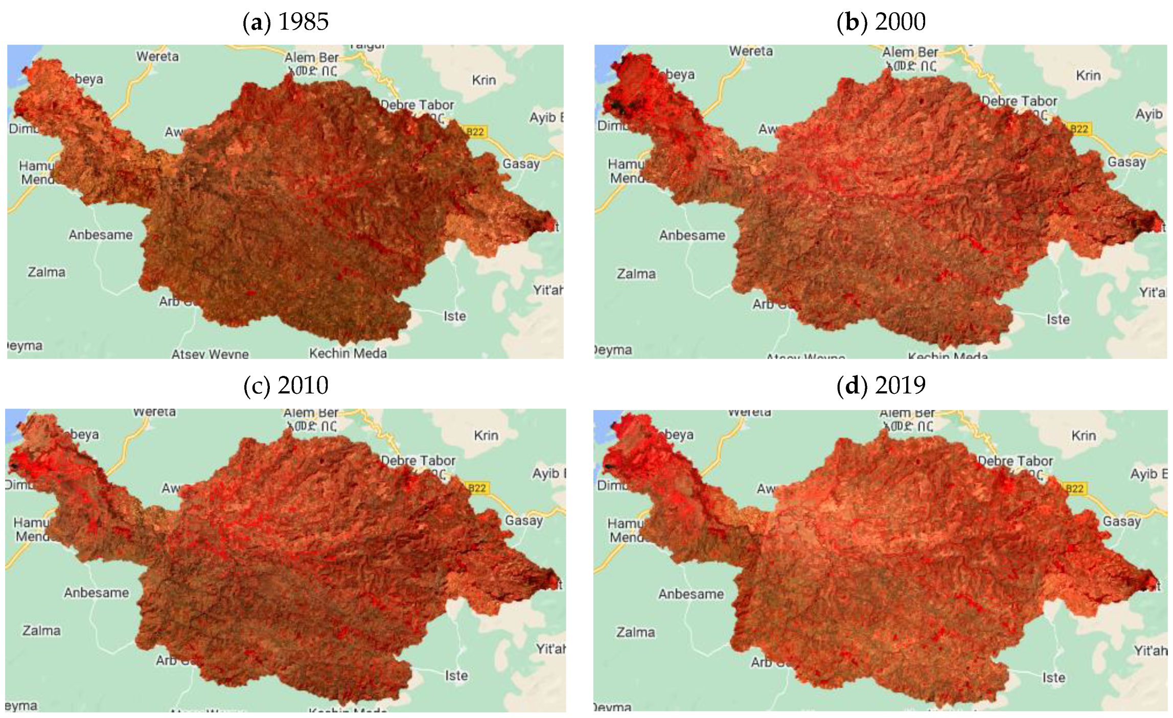
Land 13 00396 g001
Figure 2. False color composites (NIR, red and green bands) of Landsat-5/TM (ac) and Landsat-8/OLI (d) images used for LULC classification for the years (a) 1985, (b) 2000, (c) 2010, and (d) 2019. The deep red areas represent areas covered with scattered plants; the darker red areas represent densely vegetated areas.
Land 13 00396 g002
Figure 3. Methodological framework of LULC classification and change detection.
Land 13 00396 g003
Figure 4. Methodological framework for future LULC prediction.
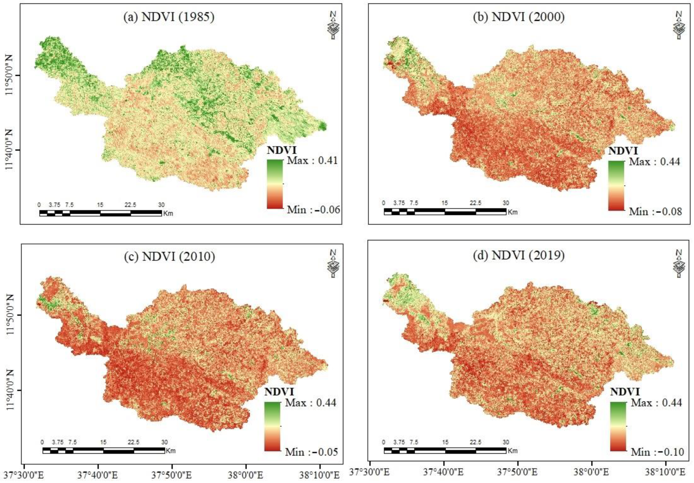
Land 13 00396 g004
Figure 5. Computed NDVI images of the Gumara watershed for the years (a) 1985, (b) 2000, (c) 2010, and (d) 2019. In the figures, dark greens (maximum NDVI values example, NDVI = 0.4) represent vegetated areas, while dark reds (minimum NDVI values) represent bare soils or agricultural lands.
Land 13 00396 g005
Figure 6. Computed SAVI images of the Gumara watershed for the years (a) 1985, (b) 2000, (c) 2010, and (d) 2019. In the figures, dark greens (maximum SAVI values, for example, SAVI ≥ 0.6) represent highly vegetated areas, while dark reds (minimum SAVIvalues) represent bare soils or agricultural lands.
Land 13 00396 g006
Figure 7. Map of driver variables: (a) elevation, (b) slope, (c) distance from streams, (d) distance from roads, (e) distance from towns, and (f) evidence likelihood.
Land 13 00396 g007
Figure 8. LULC maps of the Gumara watershed for (a) 1985, (b) 2000, (c) 2010, and (d) 2019. The values in the legend indicate the percentage of each LULC class.
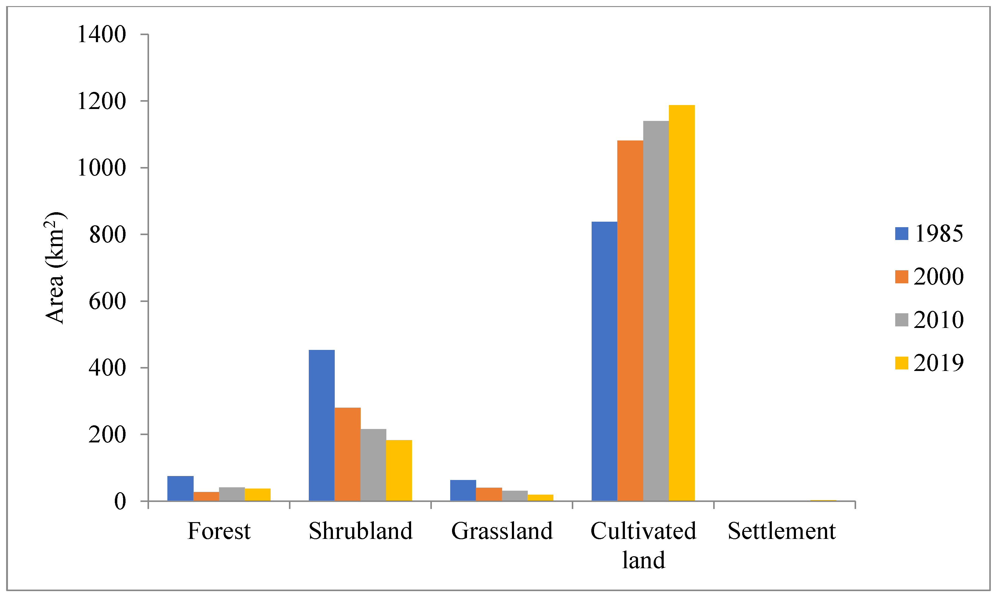
Land 13 00396 g008
Figure 9. Area of each LULC class in the Gumara watershed for the four historical years (1985, 2000, 2010, and 2019).
Land 13 00396 g009
Figure 10. (a) UA and (b) PA assessment results for each class for the LULC maps for the years 1985, 2000, 2010, and 2019.
Land 13 00396 g010
Figure 11. Relative variable importance (%) for the four datasets used for mapping LULC in the Gumara watershed: (a) Landsat-5/TM (1985), (b) Landsat-5/TM (2000), (c) Landsat 5/TM (2010), and (d) Landsat-8/OLI (2019).
Land 13 00396 g011
Figure 12. Net change (gain-loss) in each LULC class for the four study periods (1985–2000, 2000–2010, 2010–2019, and 1985–2019).
Land 13 00396 g012
Figure 13. Contribution of each LULC class to the net change in cultivated land: (a) 1985–2000, (b) 2000–2010, (c) 2010–2019, and (d) 1985–2019.
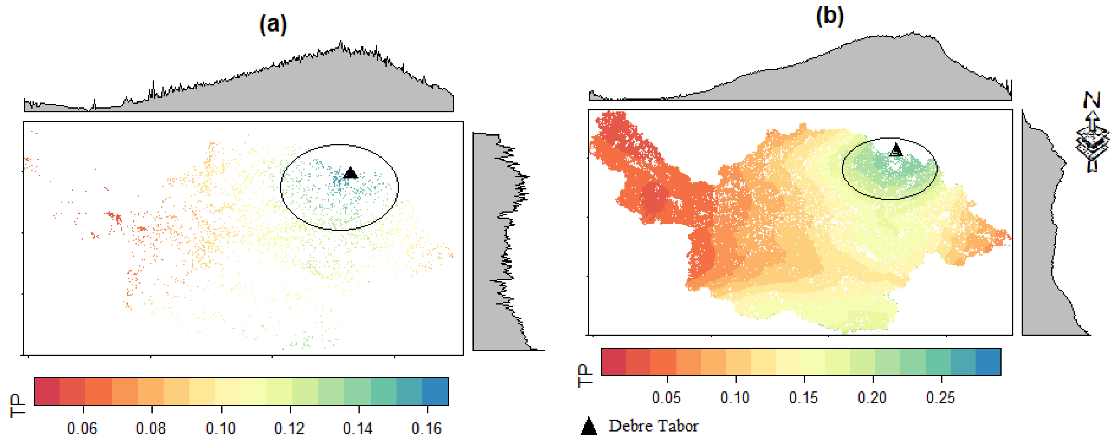
Land 13 00396 g013
Figure 14. Potential for transition: (a) shrubland to cultivated land and (b) cultivated land to settlement. TP is the transition potential. The greater the TP is, the greater the possibility of a transition from one class to another. The gray shaded regions show the orientation gradients of the transition potential, wherein the maximum transitions are oriented along the northeastern part of the watershed for both transitions. The areas bordered by circles indicate the maximum values of transition suitability. The triangle symbol in both of the figures indicates the location of the town Debre Tabor.
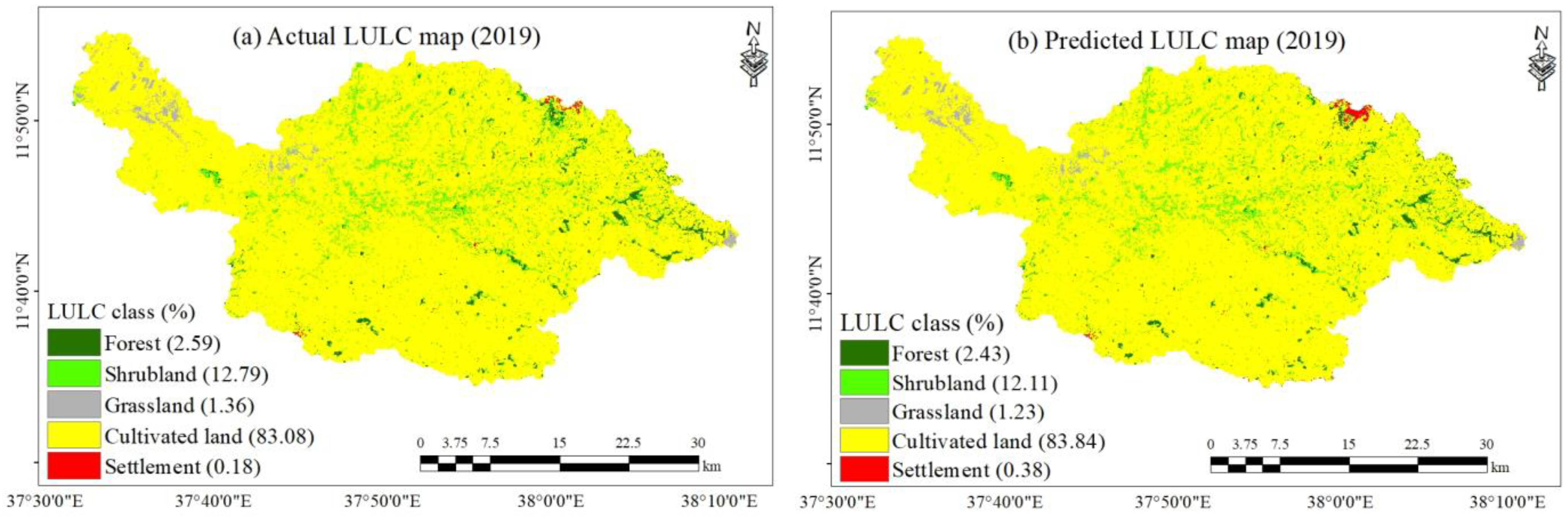
Land 13 00396 g014
Figure 15. LULC maps (2019): (a) reference LULC map and (b) CA–Markov model-predicted LULC map under the BAU scenario.
Land 13 00396 g015
Figure 16. Comparison of the reference (baseline) and predicted areas of the LULC classes in the Gumara watershed in 2019.
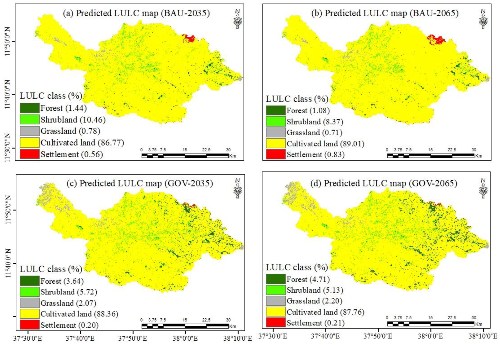
Land 13 00396 g016
Figure 17. Predicted LULC maps of the Gumara watershed: (a) for 2035 and (b) for 2065 under the BAU scenario; (c) for 2035 and (d) for 2065 under the GOV scenario.
Land 13 00396 g017
Figure 18. Net changes (gain-losses): (a) net change (2019–2065) under the BAU scenario and (b) net change (2019–2065) under the GOV scenario.
Land 13 00396 g018
Table 1. Description of Landsat surface reflectance images used for LULC classification of the Gumara watershed.
Landsat ImageDate of AcquisitionPath/RowNo. of ImageResolution (m)
Landsat-5/TM1 January–30 April 1985169/052630
Landsat-5/TM1 January–30 March 2000169/052630
Landsat-5/TM1 January–30 March 2010170/052330
Landsat-8/OLI1 January–30 March 2019169/052630
Table 2. Description of identified LULC classes in the Gumara watershed.
LULC ClassDescription
ForestAreas covered with open forest, dense forest, and woodland. This class mainly includes Eucalyptus tree and other woody plantations of the watershed.
ShrublandArea of land covered with open and closed bushes and shrubs mainly found along the banks of rivers and streams.
GrasslandAreas covered with grasslands mainly used for grazing.
Cultivated landAreas of agricultural land mainly used for crop cultivation. It also includes rice cultivation which concentrates at wetland part of the watershed.
SettlementAreas of urban and rural settlements and other developments like roads.
Table 3. Area and percentage of each LULC class in the Gumara watershed for the four historical years (1985, 2000, 2010, and 2019).
LULC ClassArea (1985)Area (2000)Area (2010)Area (2019)
(km2)(%)(km2)(%)(km2)(%)(km2)(%)
Forest74.605.2227.621.9340.772.8537.012.59
Shrubland449.4931.72280.0019.58216.0015.11182.8112.79
Grassland62.904.4039.962.7930.642.1419.471.36
Cultivated land837.7958.601077.1475.621136.1179.761184.4883.08
Settlement0.810.060.990.071.880.132.630.18
Table 4. Results of the classification accuracy assessment in terms of the overall accuracy (OA) and kappa coefficient (K).
LULC MapOverall AccuracyKappa CoefficientStatus of Agreement
198594.390.92Perfect agreement
200094.840.94Perfect agreement
201093.130.90Perfect agreement
201991.130.88Perfect agreement
Table 5. Percent change (PΔ) in (%) and annual rate of change (RΔ) in km2/year for the four study periods.
LULC Class1985–20002000–20102010–20191985–2019
Forest−62.98−3.1337.641.32−9.24−0.42−50.40−1.11
Shrubland−38.26−11.57−22.86−6.40−15.36−3.69−59.69−7.96
Grassland−36.48−1.53−23.33−0.93−36.46−1.24−69.05−1.28
Cultivated land29.0516.225.455.904.155.2641.7410.28
Settlement22.310.0139.320.0940.290.0834.860.05
Table 6. Gain and loss of each LULC class for the four study periods.
LULC Class1985–20002000–20102010–20191985–2019
Gain (km2)Loss (km2)Gain (km2)Loss (km2)Gain (km2)Loss (km2)Gain (km2)Loss (km2)
Forest4.0052.4514.581.578.4312.0111.1550.16
Shrubland91.32262.2564.17125.2056.7491.6151.74318.56
Grassland23.8746.4521.2931.169.8621.729.1553.45
Cultivated land322.2880.18139.7783.46113.4863.88399.1751.16
Settlement0.710.572.000.572.291.722.860.71
Table 7. Cramer’s V values of LULC driver variables.
Driver VariablesCramer’s Vp Value
Elevation0.21050.0000
Slope0.04370.0000
Distance from streams0.08680.0000
Distance from roads0.10040.0000
Distance from towns0.05210.0000
Evidence likelihood0.48850.0000
Table 8. (a) Transition probability matrix of LULC classes in the Gumara watershed from 1985 to 2000. (b) Transition probability matrix of LULC classes in the Gumara watershed from 2000 to 2010. (c) Transition probability matrix of LULC classes in the Gumara watershed from 2010 to 2019. (d) Transition probability matrix of LULC classes in the Gumara watershed from 1985 to 2019.
(a)
19852000
ForestShrublandGrasslandCultivated LandSettlement
Forest0.1848 10.46510.00430.34470.0010
Shrubland0.00530.28880.00870.69700.0002
Grassland0.00130.06430.25970.67470.0000
Cultivated land0.00200.06140.02180.91410.0007
Settlement0.00000.00480.00000.12080.8744
(b)
20002010
ForestShrublandGrasslandCultivated LandSettlement
Forest0.80730.08720.00170.05260.0012
Shrubland0.07100.25080.00920.66780.0012
Grassland0.00720.09970.12750.76500.0006
Cultivated land0.00450.05980.01910.91480.0018
Settlement0.00180.02480.00710.15460.8117
(c)
20102019
ForestShrublandGrasslandCultivated LandSettlement
Forest0.45710.27240.00300.26530.0022
Shrubland0.02980.21980.00590.74320.0013
Grassland0.00500.03050.16570.79780.0010
Cultivated land0.00510.04610.00870.93810.0020
Settlement0.00360.02460.00340.14340.8249
(d)
19852019
ForestShrublandForestCultivated LandForest
Forest0.58000.15260.00200.25940.0059
Shrubland0.00820.22250.00000.76910.0002
Grassland0.00060.01260.23350.75330.0000
Cultivated land0.00340.02040.00510.96990.0012
Settlement0.00160.00200.00000.47840.8180
1 The diagonal values shaded in grey colour show the proportion of the LULC classes that showed persistence (remaining unchanged).
Table 9. Predicted area and percentage of LULC classes in the Gumara watershed in 2019 and in 2035 and 2065 under the BAU and GOV scenarios.
LULC ClassReference (2019)BAU (2035)BAU (2065)GOV (2035)GOV (2065)
Area (km2)%Area (km2)%Area (km2)%Area (km2)%Area (km2)%
Forest37.012.5920.531.4415.501.0852.053.6467.304.71
Shrubland182.8112.79149.5010.46119.708.3781.745.7273.285.13
Grassland19.471.3611.120.7810.100.7129.652.0731.442.20
Cultivated land1184.4883.081236.6186.771268.6289.011259.4488.361250.8687.76
Settlement2.630.188.060.5611.900.832.930.202.960.21
Table 10. (a) Gains and losses of LULC classes between 2019 and 2065 under the BAU scenario. (b) Gains and losses of LULC classes between 2019 and 2065 under the GOV scenario.
(a)
LULC2019–20352035–20652019–2065
GainLossGainLossGainLoss
Forest0.006.720.003.140.009.86
Shrubland3.4337.872.5710.292.5744.73
Grassland0.007.290.001.000.008.29
Cultivated land48.595.1511.863.8660.459.00
Settlement5.150.023.860.059.000.02
(b)
LULC2019–20352035–20652019–2065
GainLossGainLossGainLoss
Forest26.730.0015.290.0042.020.00
Shrubland0.0120.150.058.430.0928.58
Grassland11.150.021.860.0313.010.00
Cultivated land0.0017.720.008.580.0026.30
Settlement0.000.000.000.000.010.00
Disclaimer/Publisher’s Note: The statements, opinions and data contained in all publications are solely those of the individual author(s) and contributor(s) and not of MDPI and/or the editor(s). MDPI and/or the editor(s) disclaim responsibility for any injury to people or property resulting from any ideas, methods, instructions or products referred to in the content.

