Assessment and Management Zoning of Ecosystem Service Trade-Off/Synergy Based on the Social–Ecological Balance: A Case of the Chang-Zhu-Tan Metropolitan Area

Abstract

Clarifying the trade-offs/synergies of ecosystem services is crucial for achieving a win-win situation in economic development and ecological conservation. Past studies have lacked research on ecosystem service functional management zones that integrate socio-economic factors and ecological conservation, particularly based on predictive scenarios. Based on the above, this study innovatively established a multi scenario simulation model and framework (EST-EMZ) for the study of ecosystem service (ES) trade-off/synergy and ecological management zoning, combining remote sensing and socio-economic data from 2000 to 2020 in the Chang-Zhu-Tan Metropolitan Area (CZTMA). The model evaluates the dynamic trade-offs/synergies among different ecosystem services under various scenarios, aiming to seek the optimal management approach for enhancing the functionality and optimizing the structure of ESs in the future of the CZTMA. The results indicate the following: (1) From 2000 to 2020, the Ecosystem Service Value (ESV) of the CZTMA gradually declined from 601.57 billion yuan to 584.65 billion yuan. Under the three future scenarios, the ESV also decreased, with the Ecological Conservation Scenario (ECS) experiencing the most minor decline, and the Economic Priority Scenario (EPS) witnessing the most substantial decrease. (2) In the historical period and the 2030 predicted scenarios, there is a predominant synergy among paired ESs in the CZTMA. Throughout the study period, the region’s dominant ecosystem service bundle (ESB) is the high-service ecological regulation bundle, primarily located in the northeastern, western, and southern areas dominated by forests. (3) Based on ESV and urbanization intensity (UI), five different ecosystem management zones were identified: water balance zone (WBZ), coordinated improvement zone (CIZ), ecologically weak zone (EWZ), ecological conservation zone (ECZ), and ecological derivative zone (EDZ). Corresponding management and protection strategies for ecosystem services were proposed. The research findings offer potential solutions for optimizing land use and managing the trade-offs of ESs in metropolitan areas.

1. Introduction

Metropolitan Area (MA) refers to a functional urban region with one or more central cities as the core, supported by well-developed transportation connections and closely linked to the surrounding socio-economic areas [1]. Currently, China has formed 34 MAs, which account for 50.4% of the country’s population and 65.6% of its Gross Domestic Product (GDP), making it a new strategic deployment for the high-quality development of regional urbanization. However, there are apparent contradictions between ecological growth and economic development in some MAs with the emergence of “population-land-socio-economic-ecological-environmental”compound problems [2]. Over the past 50 years, approximately 60% of ecosystem services(ESs) have been degraded or are no longer sustainably usable due to rapid and extensive human activities [3]. Furthermore, intensive human activities have directly or indirectly impacted the interactions among ESs, ultimately undermining the functionality and structural stability of ESs, leading to issues such as reduced biodiversity, declining levels of ecosystem services, and ecological degradation [4,5]. Therefore, quantifying the spatiotemporal variations and interaction relationships of ESs in urbanization is urgent and necessary for urban ecological management.

The value of ecosystem services (ESV) involves quantifying the benefits of regional ecosystem service (ES) to human society. This quantification is instrumental in decision-making processes aimed at enhancing urban well-being [6]. Due to the differences in human demand for various ESs in urbanization, there are often complex interactions among ESs. These can be summarized into two primary relationships: trade-offs and synergies [7,8]. Trade-offs refer to the conflicting or antagonistic relationships among two or more types of ESs, whereas synergies are positive interactions among two or more ESs [9]. The direction and extent of land use changes significantly impact trade-offs/synergies [10], whereas complex trade-offs/synergies profoundly affect the benefits of ecosystem services [11]. Therefore, evaluating the trade-offs/synergies among ESs contributes to optimizing regional land use management and enhancing the overall value of ecosystem services [12,13,14], which is of great significance for precisely regulating the functioning of ecosystem services in metropolitan areas and achieving a “win-win” situation for regional socio-economic development and ecological conservation [15,16,17].

Currently, research on trade-offs/synergies of ecosystem service mainly focuses on two categories of issues: first, assessing the trade-offs/synergies among ESs, analyzing their spatiotemporal characteristics, identifying bundles of ESs, and forming ecological management zones [18]; second, exploring the driving mechanisms behind the trade-offs/synergies [19,20,21,22]. For example, the driving forces include land use [23,24], climate change impacts [25], and grazing exclusion effects [26], among others. Regarding the research techniques for studying the trade-offs and synergies between paired ESs, there are mainly static and dynamic spatial correlation methods [27]. Static correlation methods mainly correlation analysis [28], static trade-off and synergy degree [29,30], and Bayesian network methods [31]. Dynamic correlation methods often use the Ecosystem Service Trade-off and Synergy Degree (ESTD) model. The trade-offs/synergies between grouped ESs are usually represented by ecosystem service bundle(ESB). They are often identified using principal component analysis [32] and bundle analysis [33]. This can reflect the combined relationships among ESs with similar functional structures and plays a crucial role in identifying and quantifying dominant types of ecosystem services [34]. Most scholars base their ecological management zoning on the results of ecosystem service bundles to emphasize the importance of the connections among ESs. However, ecological management zoning is the coordination between regional social development and ecological protection [35]. Currently, many studies overlook the spatial correlation between socioeconomics and ecosystem service in zoning, and there still needs to be a research gap in integrating the two and applying them to the future optimization of trade-offs/synergies in ecosystem management zoning.

The combination of multi-scenario land use prediction and ecosystem services’ dynamic trade-offs/synergies for robust multi-objective support for analyzing future ecological management patterns in specific areas needs to be revised. More research is needed from the perspective of land use simulation under different scenarios. The combination of multi-scenario land use prediction and ecosystem services’ dynamic trade-offs/synergies for robust multi-objective support for analyzing future ecological management patterns in specific areas needs to be revised. More research is needed from the perspective of land use simulation under different scenarios. Currently, mainstream land use prediction models include the CA-Markov model, Geo SOS-FLUS model, Artificial Neural Network model (ANN), and CLUES model. The CA model possesses robust spatial computational capabilities for simulating complex systems by analyzing spatial transformations. However, its linear analytical capabilities are relatively limited. The Markov chain model can quantitatively simulate land use transitions based on long time series of land use transfer matrices and adaptive graph sets, compensating for the shortcomings of the CA model. Therefore, combining the spatial–temporal predictive advantages, the CA-Markov model can enhance prediction accuracy, providing more informative results for the simulation of spatial-temporal evolution scenarios [36,37,38]. It offers a simple, easy-to-implement, and user-friendly approach for urban land use simulation [39], successfully applied in numerous urban studies [40,41].

To address the research gaps and limitations, this study innovatively constructs a multi-scenario simulation model and framework (EST-EMZ) for the trade-offs/synergies of ESs and ecological management zoning. The aim is to integrate ecosystem services with urbanization levels to obtain ecological management zoning guided by trade-offs/synergies, thereby supporting regional ecological service management practices. In terms of the study area, this paper selects the Chang-Zhu-Tan Metropolitan Area (CZTMA), which is the first “national-level metropolitan area” in Central China. The rapid expansion of land use has accelerated the transformation of rural landscapes into urban landscapes, leading to severe damage to the landscape pattern and ecological environment of the metropolitan area, resulting in a significant decline in the value of ecosystem service. Therefore, it is a crucial area for addressing ecosystem service management issues. In terms of the research content, the specific objectives are: (1) to reveal the spatiotemporal dynamic characteristics of land use change and changes in ecosystem service values under three projected scenarios for the years 2000, 2010, 2020, and 2030, and to explain how land use change affects ESs; (2) to evaluate the dynamic trade-offs/synergies of ESs in the CZTMA, systematically exploring the spatiotemporal differences in trade-offs/synergies effects; and (3) to integrate the trade-offs/synergies assessment results and propose optimized management strategies for different ecological management zones.

2. Materials and Methods

2.1. Study Area

The CZTMA is located in the transitional zone between the eastern and central-western parts of China and is an essential component of the urban cluster in the middle reaches of the Yangtze River (Figure 1). The total area of the study area is 18,900 square kilometers, and, according to the “Chang-Zhu-Tan Metropolitan Area Plan”, the study area includes the entire scope of Changsha, the central city district of Zhuzhou, Liling City, the central city district of Xiangtan, Shaoshan City, and Xiangtan County. The primary land use in the study area is woodland and arable land, with the Xiang River flowing from south to north through the central part of the study area. The CZTMA is the most active region in terms of construction land expansion and ecological environment change in Hunan Province, and it serves multiple ES functions such as social development, climate regulation, and cultural services. However, with rapid economic growth and the continuous expansion of urban areas, the ecological environment of the metropolitan area has been severely disturbed, resulting in an imbalance in ES functions and structure and an increasingly prominent contradiction between environmental protection and economic development.

2.2. Data Sources

The data used in this study include land use data, socio-economic data, road network data, and other data. The land use data for the study area are categorized into six types: arable land, forest land, grassland, water bodies, built-up land, and unused land, based on the land use characteristics of the study area. All geographical data were projected to WGS_1984_UTM_ZONE 50N using ArcGIS 10.2 software, and the grid calculation unit was set to 2 km × 2 km raster cells. Below are the specific data sources and specifications (

Table 1. Data Source and Specifications.

Data Categories	Specifications	Data Sources
Land Use Data (2000–2020)	Raster, 30 m × 30 m	Chinese Academy of Sciences Resource and Environmental Science Data (RESDC) “http://www.resdc.cn” accessed on 15 June 2023
DEM Data	Raster, 30 m × 30 m	Geospatial Data Cloud (https://www.gscloud.cn/) accessed on 15 June 2023
Railways (2020)	Vector, Line	OpenStreetMap (https://www.openstreetmap.org/) accessed on 15 June 2023
Major Roads (2020)	Vector, Line
Administrative Division Data	Vector, Polygon	Chinese Academy of Sciences Resource and Environmental Science Data (RESDC) “http://www.resdc.cn” accessed on 15 June 2023
Nature Reserve Data	Vector, Polygon	Nature Reserve Specimen Resource Sharing Platform http://www.papc.cn/ accessed on 16 June 2023
Chang-Zhu-Tan Green Heart Zone Data	Vector, Polygon	Hunan Provincial People’s Government website (http://www.hunan.gov.cn) accessed on 16 June 2023
Grain Production Data	Statistical, County	China Statistical Yearbook https://www.stats.gov.cn/sj/ndsj/2023/indexch.htm accessed on 16 June 2023

).

2.3. Methods

Taking CZTMA as the research object, this paper constructed a modeling framework of ES trade-off synergistic evaluation and ecosystem management zoning (EST-EMZ) (Figure 2), containing three steps: (1) Ecological value multi-scenario analysis. Firstly, we constructed a land use multi-scenario simulation atlas. Based on historical land use types, conversion limiting factors, and influencing factors, we used the CA-Markov model to obtain land use type maps for three predicted scenarios in 2030. Secondly, we generated an ESV atlas. Using raster land use data under different scenarios, we estimated the ESV under various scenarios using the value equivalent factor method, describing the spatiotemporal characteristics and evolutionary patterns of ESV. (2) Trade-off/coordinated relationship assessment: Quantify the dynamic trade-off and coordination relationship between paired ESs using the Weighted Coordinated Degree (ESTD) model. Identify ecological service clusters (ESB) through K-means clustering analysis to describe the trade-off and coordination relationships among multiple ESs. (3) Based on the ESV within each grid unit and urbanization intensity, delineated future ecological management zones in the study area through bivariate spatial autocorrelation analysis.

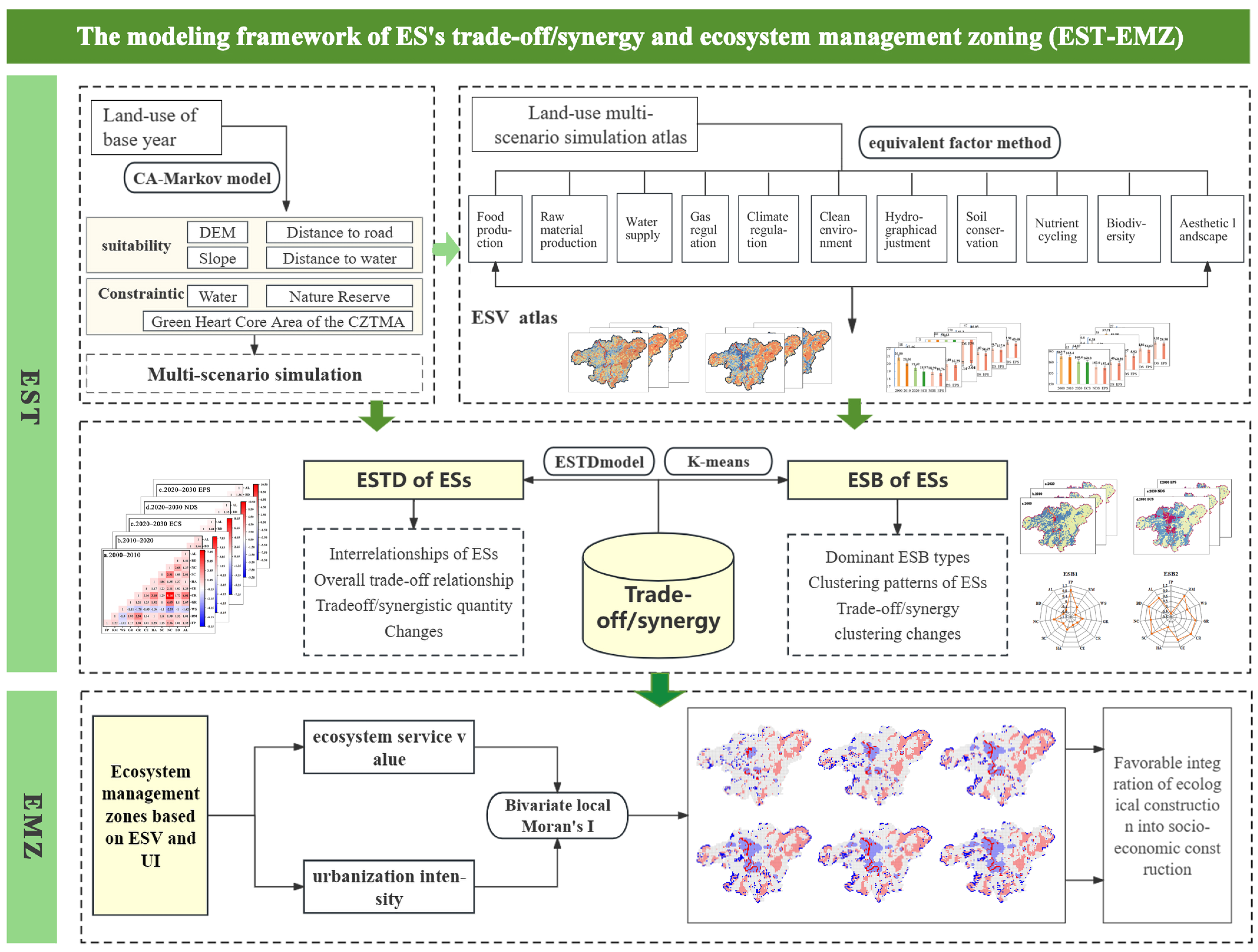
2.3.1. Land Use Multi-Scenario Simulation Atlas Construction

(1)

Obtain the land use transfer probability matrix. The Markov module in IDRISI17.0 software was used to derive the land use transfer area matrix and transfer probability matrix for the study area from 2010 to 2020, with the following formulas:

$$\begin{array}{c}{S}_{\left(t+1\right)}=S_t\times P_{ij}\end{array}$$

(1)

where $S_{\left(t+1\right)}$ is the state represented by land use at time $t$, $S_{\left(t+1\right)}$ is the momentary land use state, and $P_{ij}$ is the land use transfer matrix, calculated as follows:

$$\begin{array}{c}{P}_{ij}=\left[\begin{array}{c}{P}_{11}\cdots P_{1n}\\ ⋮⋮⋮\\ P_{n1}\cdots P_{nn}\end{array}\right]\end{array}$$

(2)

where $0\le P_{ij}<1$, and $\sum _{j=1}^n{P}_{ij}=1\left(i,j=1,2,\dots ,n\right)$; $n$ is the land use type.

The CA-Markov module, which combines the two models, can scientifically and rationally deduce the spatial change in land use pattern [42,43]. For the CA model, the calculation formula is as follows:

$$\begin{array}{c}{S}_{\left(t+1\right)}=f\left[S_{\left(t\right)},N\right]\end{array}$$

(3)

$S$ represents a set of finite discrete states of cells; $N$ represents the neighborhood of cells; $t$ and $t+1$ represent different periods; and $f$ represents the cellular transformation rules in the local space.

(2)

Create a suitability atlas, using the Decision Wizard module in the IDRISI 17.0 software for the land use transfer adaptability atlas of the study area. Considering the study area’s natural geographical features and socio-economic development status, factors such as elevation, slope, distance to roads, and distance to water bodies were comprehensively assessed and quantified as suitability factors. Water bodies, nature reserves, and the Chang-Zhu-Tan Green Heart Ecological Core Area were considered as restrictive factors in the production of the suitability atlas.

(3)

Simulation Accuracy Verification. The CROSSTAB module in IDRISI 17.0 software was employed for simulation accuracy verification. A comparison was made between the actual land use types in 2020 and the predicted land use types for the same year, and the Kappa value was computed. The resulting Kappa coefficient was 0.9116 (greater than 0.8), meeting the accuracy requirements.

While the model’s overall accuracy does not necessarily reflect the fitting degree for each land use category, additional validation of the simulation accuracy for each land class was conducted. The simulated results were compared with the actual land areas, and discrepancies were presented in

Table 2. Comparison of actual and simulated land use area in Chang-Zhu-Tan Metropolitan Area in 2020 (km²).

Land Use	Cropland	Woodland	Grassland	Water	Construction	Unused
Actual area in 2020	5690.00	11,275.33	158.47	427.78	1426.63	6.92
Simulated area in 2020	5721.25	11,325.27	157.53	430.94	1343.41	6.72
Error/%	0.55	0.44	−0.59	0.74	−5.83	−2.95

and Figure 3. The most significant error was observed in the land designated for construction, reaching 5.83%. Although there was a solid overall correspondence between the current state and the simulated map for 2020, some spatial pattern differences were noted. In Figure 3a, a portion of the construction land in 2020 was predicted to be cropland or woodland. Due to the scattered spatial distribution of construction land cells, significantly influenced by human activities, and with a relatively weaker control from natural background compared to other land classes, the simulation accuracy for construction land was relatively lower. The simulation area and spatial pattern errors are within an acceptable range, indicating that this method can be utilized for the 2030 land use simulation prediction.

(4)

Simulation of conversion scenarios and rule sets. Considering the research objectives of achieving future ecosystem and economic coordination, the patterns of land use changes in metropolitan area, and the future development plans for metropolitan area [44], this study has formulated the three most representative land use simulation scenarios. The conversion principles for each scenario are as follows (

Table 3. Conversion rules for land use types under different scenarios.

Scenario Type	Conversion Rules
Ecological Conservation Scenario (ECS)	Water, nature reserve, and part of the Green Heart area are considered constraint; conversion from high ecological value land to low ecological value land is to be limited: conversion from cropland to woodland is increased by 30%, whereas transformation from cropland, unused land, woodland, and grassland to construction land is reduced by 40% and 50%, respectively [45].
Natural Development Scenario (NDS)	Based on the land use change patterns from 2000 to 2020, there are no restrictions on the conversion between land types. It serves as the reference scenario for the forecast.
Economic Priority Scenario (EPS)	According to the land use planning texts of various cities in the CZTMA, the maximum increase in construction land is set at 50%, and nature reserve is considered a constraint. Land conversions with high economic benefits are increased: conversion from grassland, water, unused land, cropland, and woodland to construction land are increased by 30%, 40%, and 60%, respectively [46,47].

):

The probability matrices for land use conversion under three scenarios in 2030 were derived using the conversion rules and historical conversion probabilities, as shown in

Table 4. Matrix of land use conversion probabilities under different scenarios.

Scenario Setting		Cropland	Woodland	Grassland	Water	Construction	Unused
ECS	Cropland	0.7837	0.1418	0.0009	0.0093	0.0642	0.0001
	Woodland	0.1003	0.8513	0.0026	0.0045	0.0411	0.0002
	Grassland	0.0410	0.1377	0.8106	0.0026	0.0078	0.0003
	Water	0.0350	0.0243	0.0005	0.9184	0.0214	0.0004
	Construction	0.0305	0.0233	0.0001	0.0025	0.9435	0.0000
	Unused	0.0273	0.2535	0.0000	0.0281	0.0352	0.6559
NDS	Cropland	0.7738	0.1091	0.0009	0.0092	0.1069	0.0001
	Woodland	0.0960	0.8148	0.0025	0.0043	0.0822	0.0001
	Grassland	0.0407	0.1366	0.8043	0.0026	0.0156	0.0003
	Water	0.0940	0.0654	0.0013	0.7806	0.0576	0.0011
	Construction	0.1069	0.0817	0.0005	0.0089	0.8019	0.0000
	Unused	0.0266	0.2473	0.0000	0.0274	0.0586	0.6400
EPS	Cropland	0.7367	0.1039	0.0008	0.0088	0.1497	0.0001
	Woodland	0.0908	0.7711	0.0024	0.0041	0.1315	0.0001
	Grassland	0.0405	0.1359	0.8004	0.0026	0.0203	0.0003
	Water	0.0922	0.0642	0.0013	0.7663	0.0749	0.0011
	Construction	0.1069	0.0817	0.0005	0.0089	0.8019	0.0000
	Unused	0.0261	0.2427	0.0000	0.0269	0.0762	0.6280

.

2.3.2. Estimation of the ESV

Based on the Chinese ESV equivalent table calculated by Xie [48], this article adjusts the coefficient table according to the natural and social characteristics of the study area as follows: (1) adjust land use categories. Combining the actual 18 categories of secondary land use type data in the study area, take farmland as an example, and the farmland equivalent takes the average of paddy field and dry land equivalents: V_cropland = (V_dry land + V_paddy field)/2, and other land types follow suit. (2) Adjust and revise the unit value equivalent coefficient (yuan/hm²). According to various statistical yearbooks, the main grain crops in the Chang-Zhu-Tan region are rice, wheat, and corn. The total grain sowing area and yield of these three crops from 2000 to 2020 were obtained, and the grain prices were calculated using the lowest purchase prices for each produce in 2020. The value equivalent coefficient $E_a$ was estimated at 1287.26 (Formula (4)). Based on this, the biomass correction coefficient proposed by Liu Hai et al. and Yan Enping et al. [49] for Hunan Province (1.95) was used to correct the value equivalent. The final ESV equivalent coefficient $E_r$ was obtained at 2055.15 (Formula (5)).

$$\begin{array}{c}{E}_a=\frac{1}{7}{\sum }_k^n\frac{p_k{q}_k}{m_k}\end{array}$$

(4)

$$\begin{array}{c}{E}_r=E_a\times \left(\frac{Q_{CZTMA}}{2 \times Q_{NW}}+\frac{1.95}{2}\right)\end{array}$$

(5)

• where $E_a$ is the food ES per unit of farmland area (yuan/hm²), $n$ is the number of crops (n = 3), k is the type of crop, $p$ is the national minimum purchase price (yuan/kg), $q$ is the yield (yuan/hm²), and $m_k$ is the sown area of the k-th crop (hm²).
• where $E_r$ is the modified value equivalent coefficient; $Q_{CZTMA}$ and $Q_{NW}$ are the average grain yield per unit (kg/hm²) in the CZTMA and the whole country, respectively.

The ESVs for each scenario were obtained based on the area of the land use type and the value equivalent coefficients (

Table 5. The ecosystem service value coefficients of the Chang-Zhu-Tan Metropolitan Area (yuan/hm²).

ES		Cropland	Woodland	Grassland	Water	Unused
Supply Service	FP *	2270.942	518.926	479.535	1346.124	10.276
	RM *	503.512	1191.988	705.602	750.130	30.827
	WS *	−2681.972	616.545	390.479	11,180.023	20.552
Regulating Service	GR *	1829.085	3920.201	2479.883	2743.627	133.585
	CR *	955.645	11729.776	6555.933	6052.421	102.758
	CE *	277.445	3437.241	2164.759	9402.317	421.306
	HA *	3072.451	7675.990	4802.204	129,957.492	246.618
Support Service	SC *	1068.679	4773.089	3021.072	3329.345	154.136
	NC *	318.548	364.789	232.917	256.894	10.276
	BD *	349.376	4346.645	2747.052	10,707.338	143.861
Cultural Service	AL *	154.136	1906.153	1212.539	6802.551	61.655

* FP: food production; RM: raw material production; WS: water supply; GR: gas regulation; CR: climate regulation; CE: clean environment; HA: hydrographic adjustment; SC: soil conservation; NC: nutrient cycling; BD: biodiversity; AL: aesthetic landscape.

), which were calculated as follows:

$$\begin{array}{c}ESV={\displaystyle \sum _{n=1}^k}\left(A_k\times E_r\right)\end{array}$$

(6)

where $ESV$ is the ES value (yuan); $A_k$ is the area (hm²) of the k-th land use type in the study area.

2.3.3. Analysis of Trade-Off/Synergy

• Trade-off/synergy degree of paired ESs

The Ecosystem Service Trade-Off/Synergy Degree(ESTD) model established based on linear fitting can better clarify the relationship between ESs. Combined with the research of Gong et al. [50], the model is adapted to make ${ESTD}_{ij}$ unique. The specific calculation method is as follows:

$$\begin{array}{c}{ESC}_i={ES}_{iy}-{ES}_{ix}\end{array}$$

(7)

$$\begin{array}{c}{ESTD}_{ij}=\frac{1}{2}\times \left(\frac{{ESC}_i}{{ESC}_j}+\frac{{ESC}_j}{{ESC}_i}\right)\end{array}$$

(8)

• where ${ESC}_i$ is the change in the ESV of the i-th species; ${ES}_{iy}$ and ${ES}_{ix}$ are the value of ES of the i-th species at the time of $y$ and $x$, respectively.
• where ${ESTD}_{ij}$ represents the collaborative degree of balancing between the i-th and j-th ESs. Its value indicates the strength and direction of interaction between the two ESs. A value greater than 0 indicates a collaborative relationship, whereas a value less than 0 indicates a balancing relationship.

2.

Identify trade-off/synergies across multiple ESs-ESB

Cluster analysis can identify ecosystem service bundle (ESB) that embody intrinsic linkages among multiple ESs. The study used principal component analysis to determine the K value to avoid subjectivity in determining the number of clusters in the K-means algorithm. When the number of components is 4, the group’s eigenvalues tend to be stable, so the cluster (K) is taken to be 4.

2.3.4. Methodology for the Delineation of Ecosystem Management Zone (EMZ)

This study conducted a bivariate spatial Moran’s I analysis of ESs and urbanization intensity under the scenario of no change in 2030 and obtains management zones for future ESs. Using the GeoDa software version 1.22 to analyze the bivariate Moran’s I of unit grid ESV and urbanization intensity, it can express the spatial clustering relationship and degree between the two variables. Urbanization intensity(UI) is the ratio of built-up land within each cell grid to the total area of the grid, whose formula is:

$$\begin{array}{c}{UI}_i=\frac{{CA}_i}{{TA}_i}\end{array}$$

(9)

where ${UI}_i$ denotes the urbanization intensity of the i-th grid; ${CA}_i$ denotes the construction land area of the i-th grid; and $i$ denotes the total area of the i-th grid.

The bivariate spatial Moran’s I consists of the global bivariate Moran’s I (Equation (10)) and the local bivariate Moran’ I (Equation (11)). The formula is as follows:

$$\begin{array}{c}I=\frac{\sum _{i=1}^n\sum _{j=1}^n{w}_{ij}\left(x_i-\stackrel{\_}{x}\right)\left(x_j-\stackrel{\_}{x}\right)}{S^2\sum _{i=1}^n\sum _{j=1}^n{w}_{ij}}\end{array}$$

(10)

$$\begin{array}{c}{I}_i=\frac{\left(x_i-\stackrel{\_}{x}\right)\sum _{j=1}^n{w}_{ij}\left(x_i-\stackrel{\_}{x}\right)}{S^2}\end{array}$$

(11)

where $I$ and $I_i$ represent the global bivariate Moran’s I and local bivariate Moran’s I indices, respectively; $n$ is the total number of grids; $w_{ij}$ is the spatial weight matrix of $n\times n$; $x_i$ and $x_j$ represent the attribute values of two indicators in grids $i$ and $j$; and $\stackrel{\_}{x}$ and $S^2$ are the mean and variance of attribute values. The results output five types of variable relationships, no significant association and four significant correlation relationships: high-high (H-H), low-low (L-L), low-high (L-H), and high-low (H-L), where the H-L type represents the unit grid with high ESV and low UI, and so on.

2.3.5. Other Statistical Analysis Methods

In addition to spatial analysis methods, this study utilized various data statistical analysis methods, as detailed below (

Table 6. Statistical methods and descriptions.

Type	Method and Description
Land use transfer chord map	Origin 2021 Chord Diagram Module	Represents the transfer from one component to another or depicts the proportion of each component.
Unilateral ESV Bar Chart	Excel Bar Chart	Summarizes the product of the value equivalent coefficient of various Ecosystem Services (ES) and the corresponding land use area.
trade-off/synergy Heatmap	Origin 2021 Heatmap Module	Provides an intuitive understanding of the correlation between variables, revealing potential relationships among them.
Ecosystem Services Bundle Radar Chart	Excel Radar Chart	Quantifies the importance of various ES in different types of Ecosystem Service Bundles
Ecosystem Service Bundle Area Ratio Chart	Excel Line Chart	Quantifies the dominance of various ESB in different regions

):

3. Results

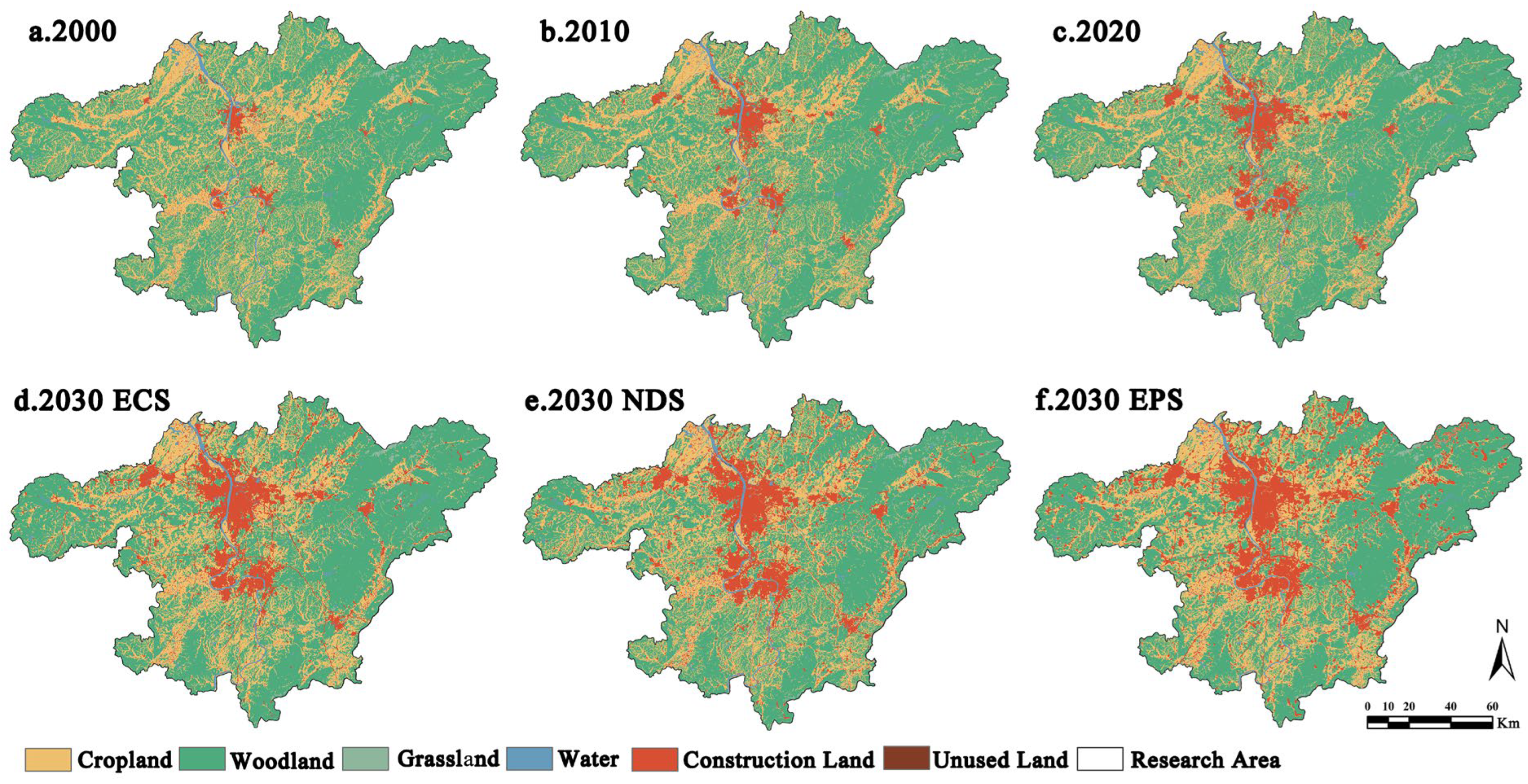
3.1. Changes in Spatial and Temporal Patterns of Land Use

From 2000 to 2020, the CZTMA witnessed rapid construction land expansion and significant spatial agglomeration effects.

(1)

Regarding proportion, the dominant land use type in the study area was woodland, accounting for approximately 60%. Cropland was the second largest, accounting for about 28%. Construction land, grassland, water, and unused land have relatively small proportions.

(2)

Regarding the trend, from 2000 to 2020, the proportion of cropland, woodland, and grassland in the CZTMA decreased. Cropland experienced the most significant decline, by 8.48%, whereas woodland and grassland decreased by 3.33% and 2.5%, respectively. Construction land increased significantly, mainly converted from cropland and woodland, with an increase of 169.87%. According to the ECS, compared to 2020, the decline in cropland and woodland slowed significantly by 3.15% and 0.9%, respectively, whereas the proportion of construction land will increase by 22.94%. According to the NDS, compared to 2020, the proportion of cropland and woodland is projected to decrease by 3.17% and 1.84%, respectively, whereas the proportion of construction land will increase by 33.23%. Under the EPS, cropland and woodland will experience significant declines, by 4.0% and 2.39%, respectively, whereas grassland and unused land will decrease by 6.9% and 9.48%, respectively. In this scenario, the probability of other land types converting to construction land is the highest, resulting in a 34.86% increase in construction land (Figure 4).

(3)

Regarding spatial distribution, cropland in the CZTMA is mainly located in the northern and southwestern parts of the study area. In contrast, woodland will mainly increase in the eastern, northern, and southern parts. Construction land is mainly distributed along the banks of the Xiang River, forming three agglomeration centers: Changsha, Zhuzhou, and Xiangtan. It expands through external transportation and gradually encroaches on surrounding ecological lands such as cropland and woodland (Figure 5).

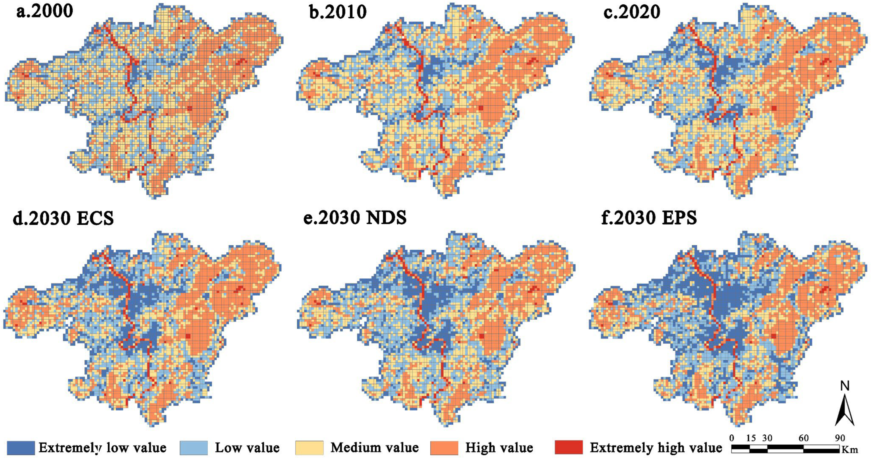
3.2. Spatial and Temporal Variations in ESV

3.2.1. Characterization of Spatial and Temporal Variations in Total ESV

According to the ESV’s coefficient table and the land use data in different scenarios in the study area, the spatial distribution of the total ESV of 2 km × 2 km grid cells in three historical years and three scenarios was obtained using the Formula (6), as well as the total ESV changes (

Table 7. Changes in ecosystem service value of the Chang-Zhu-Tan Metropolitan Area under different scenarios.

Description	Year	Land Use					Total
		Cropland	Woodland	Grassland	Water	Construction
ESV/billion yuan	2000	50.47	472.17	4.03	74.90	0.00	601.57
	2010	48.12	463.57	3.92	77.94	0.01	593.56
	2020	46.19	456.44	3.93	78.08	0.01	584.65
	2030 ECS	44.73	452.32	3.69	79.46	0.01	580.21
	2030 NDS	44.73	448.06	3.82	77.59	0.01	574.20
	2030 EPS	44.34	445.53	3.66	77.88	0.01	571.42
Rate of change/%	00–10	−4.87	−1.85	−2.76	3.90	66.35	−1.35
	10–20	−4.19	−1.56	0.19	0.18	−18.96	−1.52
	00–20	−8.48	−3.33	−2.50	4.25	149.78	−2.81
	20–30 ECS	−3.26	−0.91	−6.59	1.73	−8.51	−0.76
	20–30 NDS	−3.17	−1.84	−2.84	−0.63	1.16	−1.79
	20–30 EPS	−4.01	−2.39	−6.90	−0.26	−9.53	−2.26

ECS: Ecological Conservation Scenario; NDS: Natural Development Scenario; EPS: Economic Priority Scenario.

).

Overall, the total ESV of the CZTMA decreased by 1.692 billion yuan, or 2.81%, from 2000 to 2020. The total ESV was 60.157 billion yuan in 2000, 59.356 billion yuan in 2010, and 58.465 billion yuan in 2020, showing a continuous downward trend. Woodland contributed the most to the ESV in the study area, accounting for over 75% annually, followed by water, cropland, grassland, and unused land. Comparing the changes in ESV of various land uses, the ESV of ecological land, such as woodland and woodland, showed a decreasing trend. In contrast, the ESV of water showed a slow and continuous upward trend. Under the ECS, the increase in woodland and water slowed the decline in ESV, which decreased to 58.021 billion yuan. Under the NDS, the ESV dropped to 57.42 billion yuan, similar to the historical scenarios. Under the EPS, due to the continuous large-scale expansion of construction land, encroaching on woodland, and cropland, the ESV of the CZTMA will decrease significantly to 57.142 billion yuan.

The region with the highest ESV in the study area is located in the central Xiang River water, dominated by water and wetlands (Figure 6). The next highest value area is the peripheral mountainous region, dominated by woodland and grassland. The lower-value areas are mainly urban built-up areas, dominated by construction land and woodland. Compared to the distribution of ESVs in different scenarios, the lower value areas expanded outward from the Xiang River axis from 2000 to 2020. In the three future scenarios, due to land conversion restrictions, the EPS significantly reduced the ESV of certain ecological land, such as woodland, leading to evident degradation of ESs, with the most significant impact on woodland and cropland. In the ECS, the expansion of lower-value areas was insignificant. The reasons for the decrease in ESV are primarily attributed to the expansion of urban built-up land and the intensified human activities. The decline in the woodland’s ecosystem service contribution value has resulted in a noticeable decrease in ESV.

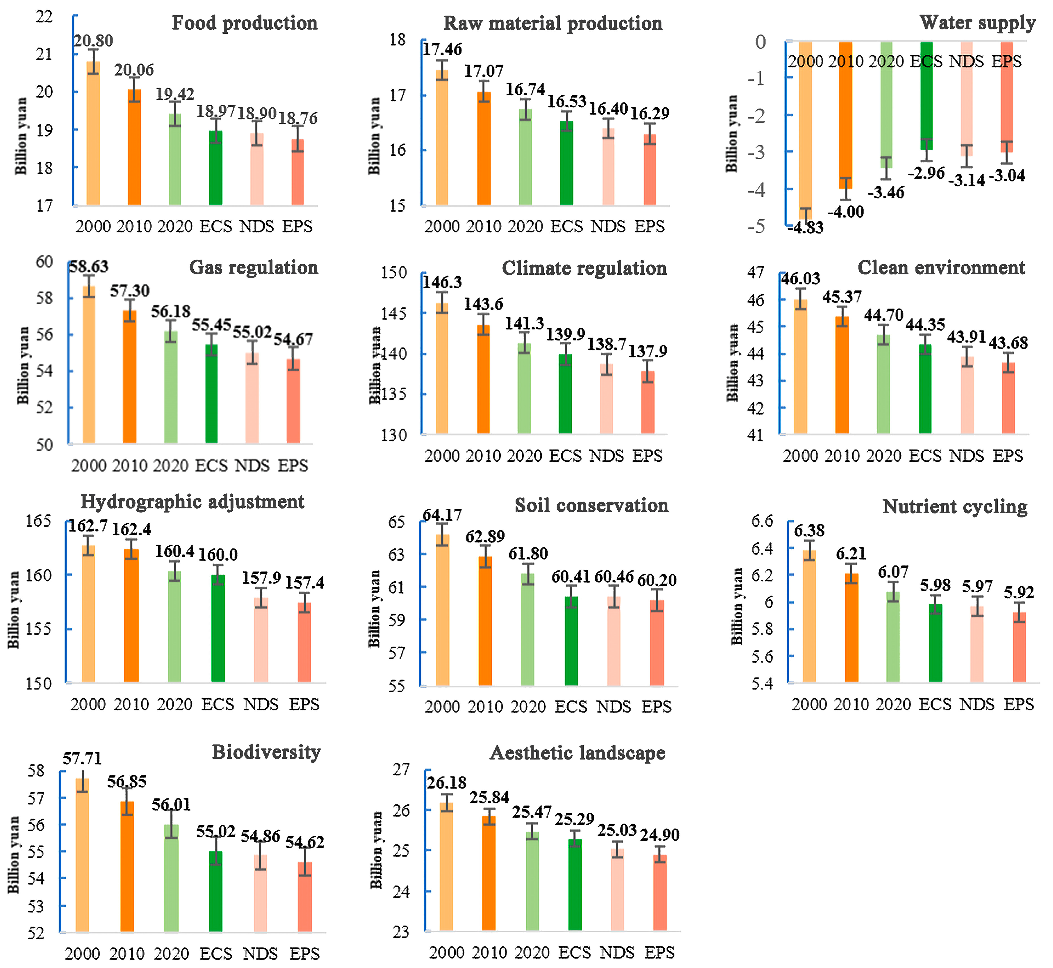
3.2.2. Characterization of Changes in Individual ESV

From 2000 to 2020, the CZTMA experienced varying degrees of decline in ESVs, except for WS, which hurt the total weight but with a gradually weakening effect (Figure 7). Among them, the value of FP experienced the most significant decline, dropping from 2.08 billion yuan to 1.942 billion yuan, a decrease of 6.62%. The value of the WS decreased by 137 million yuan, a growth rate of 28.3%, mainly due to the consumption of water resources caused by the occupation of a large amount of cropland during urban expansion. Compared to 2020, all ESVs will decrease except for HA in the three future scenarios. As woodland is the high-value land type in the study area, woodland degradation will go down slowly under the ECS, resulting in the smallest decline in individual ESV. The NDS has the second-largest drop, whereas the EPS is going to experience the most significant reduction. The value of WS will increase in all three scenarios, with the most significant addition in the ECS at 14.4% and the smallest increase in the NDS at 9.35%.

Regarding the composition of ESs, HA, CR, and SC are the top three in proportion, accounting for 27%, 24%, and 11% of the total value, respectively. HA, CR, SC, GR, and CE are the primary ESs in the CZTMA, representing regulating and supporting services. These characteristics align with the development concept of creating an urban ecological forest belt in the study area, where the Green Heart is the focus.

3.3. Trade-Off/Synergy of ES

3.3.1. ESTD between ESs

Using the ESTD model, representing the dynamic trade-of/synergistic relationship between two ESs, Formulas (7) and (8) were used to analyze the correlation between 11 ESs under different scenarios, obtaining the trade-off/synergistic relationships between each pair.

In total, 275 relationships were formed among the various ESs in different scenarios, with 50 trade-off relationships, accounting for approximately 18.18%, and 225 synergistic relationships, accounting for approximately 81.82%. It indicates that the ESs in the CZTMA were mainly synergistic during the study period (Figure 8). The trade-off/synergistic relationships between the various ESs under different scenarios do not transform, only the intensity of their effects changes. Each year, there were ten trade-off relationships and 45 synergistic relationships. The trade-off relationships mainly existed between WS and other ESs. From 2000 to 2010, the strongest trade-off was observed between WS and NC (−2.59). From 2010 to 2020, the strongest trade-off was between WS and CR (−2.24). In the ECS 2020, the strongest trade-off existed between WS and NC (−2.73). In the NDS from 2020, the highest trade-off was between WS and HA (−3.95). In the EPS 2020, the highest trade-off was between WS and CR (−4.1). Regarding synergistic relationships, the most potent synergy always existed between CR and NC, with synergistic levels ranging from 7.34 to 9.97. Overall, on the one hand, due to years of economic expansion activities, the climate regulation capacity has degraded, leading to an overall increase in the balance of trade-offs. On the other hand, with the increase in agricultural activities, the likelihood of trade-offs in soil and water conservation and hydrological regulation has significantly increased.

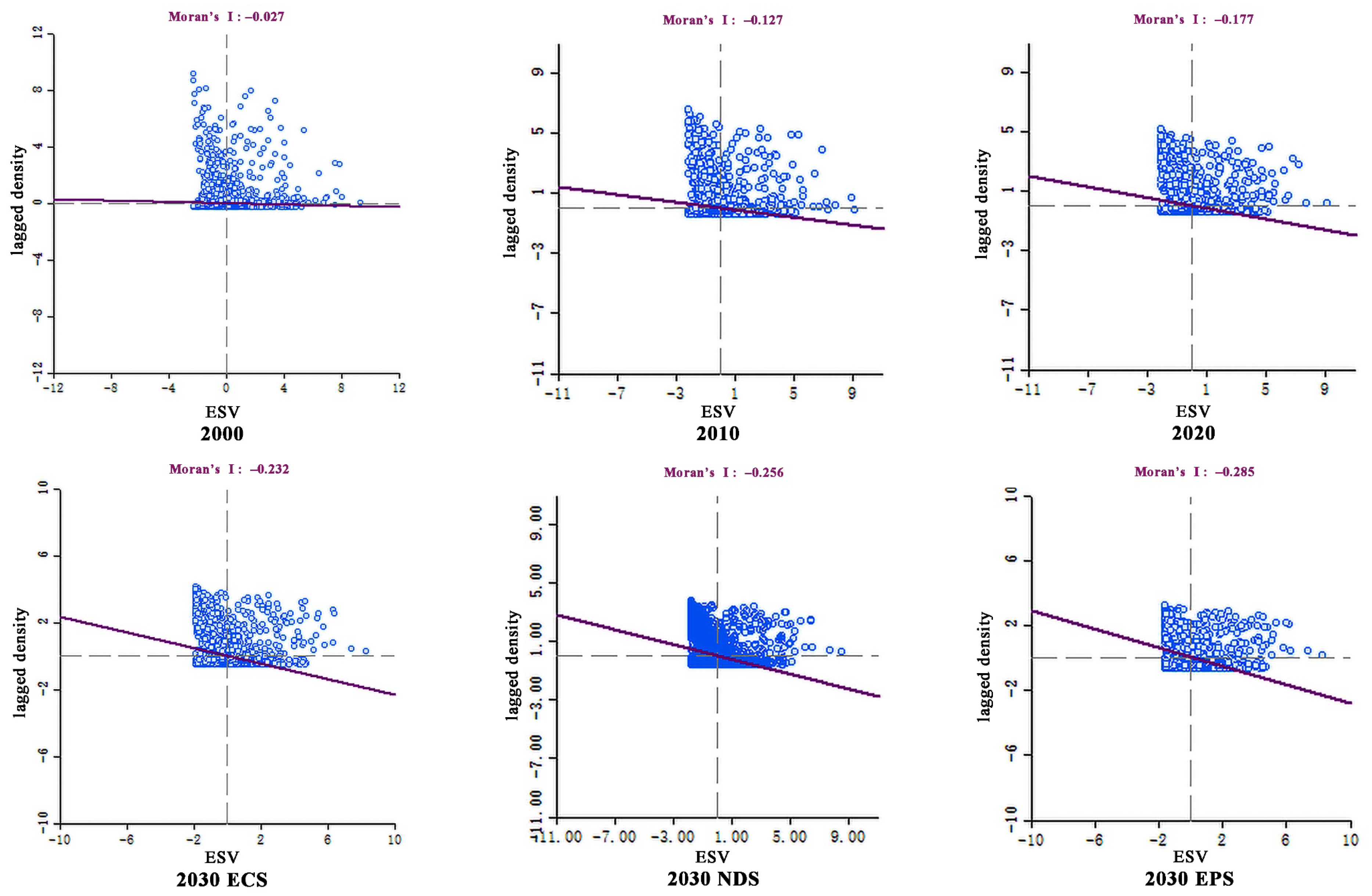
3.3.2. Spatial and Temporal Changes in ESB

Using a principal component analysis to determine the number of service clusters within the 5043 grid units in the study area by SPSS 26.0 software, the analysis revealed four ESBs. We used K-means clustering analysis to examine the spatiotemporal distribution of ESBs and their functional and structural characteristics in the CZTMA.

The CZTMA produced a total of four ESBs, and the spatial distribution of the ESBs varies significantly (Figure 9). Over the study period, the spatial distribution patterns of the four ESBs exhibited significant changes, which will differ slightly under different future scenarios. ESB1 exhibited a widespread distribution, covering almost the entire study area. It was primarily located in the urban development fringe areas, dominated by cropland. The main ecological functions of ESB1 included food production (FP), nature conservation (NC), and habitat availability (HA), making it a crucial provider of agricultural services in the study area. ESB2 was predominantly found in the eastern, northeastern, western, and southern forested areas. The land use in these regions mainly comprised woodland and grassland. The correlation coefficients of all ESs in ESB2 are relatively balanced. Its ecological functions are mainly CR, SC, RM, GR, and BD. It played a significant role in providing high-level ecological regulation services in the study area. ESB3 was primarily located in the central urban areas, consisting of construction land and wetlands. Its ecological function was mainly WS, with solid water consumption capacity but limited regulation ability. ESB3 had a relatively low ESV and a relatively simple composition of ecological functions, making it an ecologically fragile area of the city. ESB4 was mainly concentrated in the inland river and lake areas within the built-up zones—the land use in these areas mainly comprised water and wetlands. The main ecological functions of ESB4 included HA, WS, and AL, making it an essential provider of waterfront ecological recreation services in the CZTMA. The spatiotemporal variations in ESB1, ESB2, and ESB3 under different scenarios over the study period revealed the complex relationships among multiple ESs. They demonstrated the influence of land use changes and ecological management policies on different ESBs. Between 2000 and 2010, rapid urbanization in the CZTMA led to the conversion of some woodland into built-up land, resulting in a significant overall decline in ecosystem service value. However, from 2010 to 2020, with the implementation of the “Two-Oriented Society” and “Three Highs Four News” strategies in the CZTMA, efforts were made to control the expansion of built-up land, implement measures such as reforestation and returning farmland to forest, and strengthen the protection of the ecological environment. This phenomenon was alleviated during this period.

Changes in the area of each type of ecosystem service bundle from 2000 to 2020 are evident. ESB1 and ESB2 showed a gradual decrease in proportion, ranging from 37.3% to 38.6% and 47.9% to 51.4%, respectively. ESB2 had the most significant proportion among all ESBs. ESB3 showed an increasing trend, from 7.3% to 11.5%. ESB4 had the most minor proportion change, ranging from 3.3% to 4.0%. Under the ECS, forest area increased, and vegetation in key ecological areas recovered due to increased efforts in ecological protection. As a result, ESB2’s proportion slightly increased in 2020 and expanded in wetland areas. ESB3’s proportion increased by 6.74% compared to 2020. Under the NDS, the trend in service cluster changes was similar to that of the historical scenario. ESB2’s proportion increased by 12.44% compared to 2020. Under the EPS, ESB1’s proportion decreased by 17.1% compared to 2020 due to the significant construction land expansion. ESB3’s proportion significantly increased, with a growth rate of 21.42%. The growth was particularly evident in the eastern and southern central urban areas of Changsha, the northwest of Ningxiang City, the Gugang Town of Liuyang City, the western bank of Xiangjiang River in the central urban area of Zhuzhou City, the northwest of Liling City, and the northeast of the central urban area of Xiangtan City.

3.4. Identification of EMZ

3.4.1. Tests of Significance

The spatial correlation between ESV and UI was explored through bivariate Moran’s I analysis using Equations (9)–(11), aiming to identify the spatial relationship and ecological management zones. ESV and UI had a significant negative spatial correlation (Figure 10). The Moran’ I coefficients for all years were negative, ranging from −0.027 to −0.177. The degree of negative correlation gradually increased over time from 2000 to 2020. To validate the confidence of the results, all Moran’s I results were subjected to 999 random permutations. The resulting p-values were consistently 0.001, which is less than 0.05. The corresponding Z-values ranged from −5.3277 to −51.4944, falling below −2.58 (indicating a 99% significance level). Therefore, there is a significant correlation between the two variables.

Among the three future scenarios, the degree of negative correlation, compared to 2020, was highest in the EPS (−0.285), followed by the natural development scenario (−0.256) and the ECS (−0.232). Overall, the counterbalance between the intensity of urbanization and the ESV in the CZTMA is becoming increasingly apparent. This reflects the negative impact of the expansion of built-up land and human activities on the functionality and structure of ecosystem services. Simultaneously, ecological resources have suffered a certain degree of degradation, reducing the ESV of the metropolitan area and altering the balance relationships among ESs.

3.4.2. Ecological Management Zone Pattern Characteristics and Development Decisions

The overall spatial clustering characteristics between ESV and UI were significant (Figure 11). Given a clear understanding of the impact of land use changes in the CZTMA and the associated policies on the structure, function, and interrelationships of ESs, future development strategies for different management zones are proposed.

Cluster type I in the ecological management zone reveals a high-high type, the Water Balance Zone (WBZ), mainly distributed in water bodies and wetland areas within urban built-up areas. The dominant service bundle type is ESB4, accounting for approximately 46%. From 2000 to 2020, the area of this zone increased marginally from 1.6% to 2.28%. In 2030, the area is projected to increase in all three scenarios, with the highest growth observed under the Ecological Conservation Scenario ECS, projecting a 14.78% increase. The ESV in this zone is positively correlated with the intensity of urbanization, showcasing superior socio-economic and high-quality ecological development capabilities. This is primarily due to increased urban construction efforts in waterfront areas and ecological restoration, leading to an increase in water area that drives the rise in ESV. Future efforts should focus on strengthening the construction of water network functions and structures, enhancing the overall connectivity of water bodies. Building upon this foundation, a gradual transition towards high-quality eco-tourism and boutique cultural and tourism industries can be made. For example, within the metropolitan area, initiatives such as creating the Xiang River Hundred Miles Gallery scenic belt, the Island Belt in the Middle of the River, and distinctive wetland park landscapes can be developed as part of the ecological cultural tourism industry.

Cluster type II in the ecological management zones exhibited a low-low clustering pattern and can be referred to as the Coordinated Improvement Zone (CIZ). It is mainly distributed in the transitional zone between cropland and forest at the edge of towns, with the dominant ESBs type being ESB1 and ESB3. In 2030, under all three scenarios, the area of this zone is projected to increase. ESV in this zone decreased with the decrease in UI, mainly due to the random occupation of ecological lands such as cropland land and forest in remote areas during the rapid urbanization process, leading to extensive development and ultimately resulting in the “double defeat” of economy and ecology. In future management practices, more significant consideration should be given to ecological restoration projects, such as afforestation and land reclamation. While ensuring the safety of the regional ecological environment, there should be increased investment in land improvement and the development of ecological agriculture to promote soil conservation functions in the area.

Cluster type III in the ecological management zones exhibited a low-high clustering pattern and can be referred to as the Ecologically Weak Zone (EWZ). It is mainly distributed in areas prone to human disturbance, such as urban built-up and newly built urban areas, mainly consisting of construction land and surrounding cropland. The dominant ESB changed from ESB1 to ESB3, with the proportion of ESB1 decreasing from 63.9% in 2000 to 37.7% in 2020 and the area of ESB4 increasing dramatically from 30.2% to 60.6%. It indicates that a large amount of cropland has been converted into construction land in this region over the long time series. The ecosystem composition and structure exhibit instability, and the regulatory capacity is relatively weak. This has led to a change in the dominant service bundle type and a subsequent decline in the ESV. Therefore, the trend in this zone is still one of growth by 2030, with a 48.67% increase projected under the economic priority scenario. Improvement can be achieved through compact land use, green building practices, sustainable transportation, urban microclimate management, and stormwater management systems. Cluster type IV of the EMZ was a high-low clustering pattern and can be called the Ecological Conservation Zone (ECZ). It is mainly distributed in the eastern forest zone of the study area, with land types mainly consisting of forest and grassland. From 2000 to 2020, the dominant ESB in this zone was ESB2, accounting for as high as 95%. This zone had a high ESV, balanced functionality, relatively stable structure, and beautiful ecological space, playing an important role in ecological security. However, influenced by urbanization, the proportion of ESB2 slowly decreased over time.

Cluster type IV in the ecological management zones exhibited a high-low clustering pattern and can be called the Ecological Conservation Zone (ECZ). It is mainly distributed in the eastern forest zone of the study area, with land types mainly consisting of forest and grassland. The ESV in this region is relatively high, with balanced functions and a relatively stable structure. It plays a crucial role in ecological security, making it a key area for management and protection [51]. However, due to the influence of urbanization, the area proportion of this type of zoning slowly decreases over time. In the future development process, it is crucial to strengthen forest conservation and create east–west ecological forest belts from Pingtang to Zhaoshan, Shiyanshu, and Yunfeng Lake, as well as north–south ecological forest belts from Yisu River to Fahua Mountain, Shiyanshu, and Tiaoma and create diverse habitats to enhance the synergistic effects among biodiversity and ESs.

Cluster type V in the ecological management zones exhibited a non-significant correlation pattern and can be referred to as the Ecological Derivative Zone (EDZ). It is mainly distributed in the mixed zone between agriculture and forest, with complex land types, mainly consisting of cropland and woodland and the dominant ESBs being ESB1 and ESB2, accounting for approximately 45% and 43% from 2000 to 2020, respectively. In 2030, the area will decrease in all three scenarios. The management strategy for this region should focus on both ecosystem protection and a sustainable agricultural economy [52]. On the one hand, it is essential to prioritize the bottom line of farmland for food supply, improve the integration of agriculture and forestry, enhance land productivity, and ensure the sustainability of its dominant function. On the other hand, reducing human disturbances in certain transitional development areas is necessary by adjusting the planting structure of farmland and forests through ecological corridors, land restoration, afforestation, and other measures. It can enhance nutrient cycling (NC) and biodiversity (BD) benefits while ensuring food supply.

4. Discussion

4.1. The Response of Ecosystem Service Trade-Offs/Synergies to Land Use Changes

This study aims to guide future ecosystem management and promote regional ecological and economic balance by developing a trade-off/synergistic relationship assessment and zoning identification modeling framework (EST-EMZ) of the CZTMA. The results under different scenarios indicated significant heterogeneity in the ecological system trade-off/synergy of the CZTMA over time and space [53]. As urban land expansion occurs, the trade-off relationships among ecosystem services become increasingly prominent. This aligns with findings in other major metropolitan areas in China [54,55,56]. Compared to 2020, the ecosystem service value (ESV) shows a declining trend in all three future scenarios. Compared to the Natural Development Scenario, the overall ESV and individual ESVs decline more gradually in the Ecological Conservation Scenario, whereas, in the Economic Priority Scenario, both decrease more rapidly. This is consistent with the conclusions of Li et al. [57] but differs from the results of Ou et al. [58], possibly related to variations in scenario prediction conditions.

Additionally, considering the spatial aggregation of ecosystem services and the consistency of trade-off/synergy effects, this study identified four ecosystem service bundles (ESB) types. Regarding spatial distribution, ESB3, representing urban expansion, exhibits a trend of outward diffusion from the center. ESB1, representing agricultural production mainly consisting of cropland services, is distributed on the periphery of ESB3. ESB2, representing ecological conservation services primarily composed of woodland, is mainly distributed on the periphery of ESB1. This finding is consistent with the spatial distribution of ESB observed in most studies [55,59,60,61,62]. Similar to most studies, the CZTMA ecosystem services are mainly synergetic [61], and the trade-off relationships of ecosystem services primarily occur between water resource supply and other services. This is mainly due to the extensive demand for water resources from a large amount of farmland in the study area and the widespread distribution of ESB1 dominated by farmland, leading to water scarcity. Therefore, enhancing the synergy between food production, raw material production, and water supply in productive agricultural areas is crucial for the future development of the CZTMA.

4.2. A Multi-Scenario Simulation Zoning Framework Guided by Socio-Ecology Balance Orientation

The primary innovation of this study lies in emphasizing the coordinated development of ecosystem services under the framework of social–ecological balance. Integrating CA-Markov multi-scenario forecasting and bivariate spatial autocorrelation is crucial, fostering the optimization of ecosystem service functions and structure. This integration aims to improve land use management patterns and achieve effective ecological management zoning. Compared with most analyses based on ecosystem service bundle type [18,52,63], this study evaluates the relationships of ecosystem service trade-offs/synergies. After understanding the impact mechanisms of land use changes on these relationships, the study guides future zoning based on the spatial correlation between urbanization intensity (UI) and ecosystem service value (ESV) indicators for each grid. It calculates the dominant Ecosystem Service Bundles in different zones to understand each zone’s predominant ecosystem service types. Finally, based on the historical evolution patterns of management zones and current issues, the study promotes enhancing individual ecosystem service functions and overall ESV through structural regulation of land use and ecological policies. It provides a modifiable framework for future development [64,65,66]. This complex integrated study explores ecosystem services from both a “bottom-up” and a “top-down” perspective, addressing the shortcomings of previous methods that relied on a single ecological function as the basis for zoning. It fills the gap in the ecological management zoning of the Chang-Zhu-Tan Metropolitan Area. It provides a reference for studying ecosystem services in other growing metropolitan areas in Central China.

4.3. Limitations and Prospects

This study primarily focuses on the trade-off/synergy among ecosystem services (ESs). It proposes regional management policies from the perspective of the coordinated development of socioeconomics and ecology. While the study has certain limitations in widespread application, future improvements can be made in the following aspects: (1) Urbanization is a complex process involving social, economic, ecological, and policy factors. This study only analyzed the characteristics of changes in ESs under urban expansion from the perspective of land use change. Future research can supplement the analysis of various driving factors (such as population density, transportation, carbon emissions, etc.) influencing ESs [67,68]. (2) This paper only studied ESs’ multi-dimensional trade-off/synergistic relationships. However, there still needs to be more analysis on the supply demand relationship of ecosystem services and the policy analysis of supply demand coordination between different zones. It is necessary to provide a more comprehensive understanding of the evolution of ESs in the future [69]. (3) Simulating multiple scenario conditions requires high-precision data and parameters. The data collected in this study (such as socio-economic and road traffic data) still need improvement in accuracy and precision, which is one of the areas that needs to be addressed in the future. (4) Management policies for different zones can also be developed from the perspective of administrative units, based on bivariate local Moran’s l analysis, to improve the ecosystem management framework at different scales within the metropolitan area [70].

5. Conclusions

This study established a framework for assessing and managing ecosystem service (ES) trade-offs/synergies, providing a practical foundation for ecological management in the Chang-Zhu-Tan Metropolitan Area (CZTMA). The main conclusions are: ① The ecosystem service value (ESV) gradually decreases over time. ② Spatial–temporal variations in trade-offs/synergies are evident. Most of the 11 ESs in CZTMA exhibit synergistic relationships, with trade-offs primarily occurring between water supply (WS) and other types of ESs. The dominant Ecosystem Service Bundle (ESB) is the high-service forest regulation bundle. ③ Adjusting the land use structure of ecosystem management zones can enhance the ecosystem service function and provide references for solving the key problems of social and ecological conflicts in metropolitan areas. The innovation of this study lies in its social-ecological balance orientation, utilizing a research methodology that combines CA-Markov multi-scenario forecasting and bivariate spatial autocorrelation. This provides a feasible model framework for the CZTMA to optimize ecosystem service trade-off relationships, strengthen land use management patterns, establish effective ecological management zones, and offer new potential insights for other rapidly growing metropolitan areas. However, the study has limitations in widespread application, and future research could explore the multifaceted driving mechanisms of ecosystem service trade-offs related to factors such as population density, transportation, carbon emissions, and nature. Additionally, improving data accuracy and precision and formulating management policies at different scales in metropolitan areas are critical for future research.

References

1. Scott, A.J. Globalization and the rise of city-regions. Eur. Plan. Stud. 2001, 9, 813–826. [Google Scholar] [CrossRef]
2. Fang, C.L.; Liu, H.M.; Wang, S.J. The coupling curve between urbanization and the eco-environment: China’s urban agglomeration as a case study. Ecol. Indic. 2021, 130, 108107. [Google Scholar] [CrossRef]
3. Reid, W.; Mooney, H.; Cropper, A.; Capistrano, D.; Carpenter, S.; Chopra, K. Millennium Ecosystem Assessment. Ecosystems and Human Well-Being: Synthesis; Island Press: Washington, DC, USA, 2005. [Google Scholar]
4. Xiao, R.; Lin, M.; Fei, X.F.; Li, Y.S.; Zhang, Z.H.; Meng, Q.X. Exploring the interactive coercing relationship between urbanization and ecosystem service value in the Shanghai–Hangzhou Bay Metropolitan Region. J. Clean. Prod. 2020, 253, 119803. [Google Scholar] [CrossRef]
5. Xing, L.; Xue, M.G.; Hu, M.S. Dynamic simulation and assessment of the coupling coordination degree of the economy–resource–environment system: Case of Wuhan City in China. J. Environ. Manag. 2019, 230, 474–487. [Google Scholar] [CrossRef]
6. Costanza, R.; d’Arge, R.; de Groot, R.; Farber, S.; Grasso, M.; Hannon, B.; Limburg, K.; Naeem, S.; O’Neill, R.V.; Paruelo, J.; et al. The value of the world’s ecosystem services and natural capital. Nature 1997, 387, 253–260. [Google Scholar] [CrossRef]
7. Bennett, E.M.; Peterson, G.D.; Gordon, L.J. Understanding relationships among multiple ecosystem services. Ecol. Lett. 2009, 12, 1394–1404. [Google Scholar] [CrossRef] [PubMed]
8. De Groot, R.S.; Alkemade, R.; Braat, L.; Hein, L.; Willemen, L. Challenges in integrating the concept of ecosystem services and values in landscape planning, management and decision making. Ecol. Complex. 2010, 7, 260–272. [Google Scholar] [CrossRef]
9. Haase, D.; Schwarz, N.; Strohbach, M.; Kroll, F.; Seppelt, R. Synergies, Trade-offs, and Losses of Ecosystem Services in Urban Regions: An Integrated Multiscale Framework Applied to the Leipzig-Halle Region, Germany. Ecol. Soc. 2012, 17, 170322. [Google Scholar] [CrossRef]
10. Hao, J.-Y.; Zhi, L.; Li, X.; Dong, S.-K.; Li, W. Temporal and spatial variations and the relationships of land use pattern and ecosystem services in Qinghai-Tibet Plateau, China. Ying Yong Sheng Tai Xue Bao J. Appl. Ecol. 2023, 34, 3053–3063. [Google Scholar] [CrossRef]
11. Liu, J.; Pei, X.; Zhu, W.; Jiao, J. Understanding the intricate tradeoffs among ecosystem services in the Beijing-Tianjin-Hebei urban agglomeration across spatiotemporal features. Sci. Total Environ. 2023, 898, 165453. [Google Scholar] [CrossRef]
12. Austrheim, G.; Speed, J.D.M.; Evju, M.; Hester, A.; Holand, O.; Loe, L.E.; Martinsen, V.; Mobæk, R.; Mulder, J.; Steen, H.; et al. Synergies and trade-offs between ecosystem services in an alpine ecosystem grazed by sheep—An experimental approach. Basic Appl. Ecol. 2016, 17, 596–608. [Google Scholar] [CrossRef]
13. Kumar, P.; Esen, S.E.; Yashiro, M. Linking ecosystem services to strategic environmental assessment in development policies. Environ. Impact Assess. Rev. 2013, 40, 75–81. [Google Scholar] [CrossRef]
14. Harmáčková, Z.V.; Vačkář, D. Modelling regulating ecosystem services trade-offs across landscape scenarios in Třeboňsko Wetlands Biosphere Reserve, Czech Republic. Ecol. Model. 2015, 295, 207–215. [Google Scholar] [CrossRef]
15. Agudelo, C.A.R.; Bustos, S.L.H.; Moreno, C.A.P. Modeling interactions among multiple ecosystem services. A critical review. Ecol. Model. 2020, 429, 109103. [Google Scholar] [CrossRef]
16. Tian, P.; Liu, Y.C.; Li, J.L.; Pu, R.L.; Cao, L.D.; Zhang, H.T. Spatiotemporal patterns of urban expansion and trade-offs and synergies among ecosystem services in urban agglomerations of China. Ecol. Indic. 2023, 148, 110057. [Google Scholar] [CrossRef]
17. Jin, M.; Han, X.L.; Li, M.Y. Trade-offs of multiple urban ecosystem services based on land-use scenarios in the Tumen River cross-border area. Ecol. Model. 2023, 482, 110368. [Google Scholar] [CrossRef]
18. Mo, W.; Zhao, Y.; Yang, N.; Xu, Z. Ecological function zoning based on ecosystem service bundles and trade-offs: A study of Dongjiang Lake Basin, China. Environ. Sci. Pollut. Res. 2023, 30, 40388–40404. [Google Scholar] [CrossRef]
19. Zheng, H.; Wang, L.J.; Wu, T. Coordinating ecosystem service trade-offs to achieve win–win outcomes: A review of the approaches. J. Environ. Sci. 2019, 82, 103–112. [Google Scholar] [CrossRef]
20. Feng, Q.; Zhao, W.W.; Duan, B.L.; Hu, X.P.; Cherubini, F. Coupling trade-offs and supply-demand of ecosystem services (ES): A new opportunity for ES management. Geogr. Sustain. 2021, 2, 275–280. [Google Scholar] [CrossRef]
21. Pan, N.H.; Guan, Q.Y.; Wang, Q.Z.; Sun, Y.F.; Li, H.C.; Ma, Y.R. Spatial Differentiation and Driving Mechanisms in Ecosystem Service Value of Arid Region: A case study in the middle and lower reaches of Shule River Basin, NW China. J. Clean. Prod. 2021, 319, 128718. [Google Scholar] [CrossRef]
22. Wang, L.J.; Zheng, H.; Wen, Z.; Liu, L.; Robinson, B.E.; Li, R.N.; Li, C.; Kong, L.Q. Ecosystem service synergies/trade-offs informing the supply-demand match of ecosystem services: Framework and application. Ecosyst. Serv. 2019, 37, 100939. [Google Scholar] [CrossRef]
23. Wu, J.X.; Zhao, Y.; Yu, C.Q.; Luo, L.M.; Pan, Y. Land management influences trade-offs and the total supply of ecosystem services in alpine grassland in Tibet, China. J. Environ. Manag. 2017, 193, 70–78. [Google Scholar] [CrossRef] [PubMed]
24. Zhao, Y.N.; Wang, M.; Lan, T.H.; Xu, Z.H.; Wu, J.S.; Liu, Q.Y.; Peng, J. Distinguishing the effects of land use policies on ecosystem services and their trade-offs based on multi-scenario simulations. Appl. Geogr. 2023, 151, 102864. [Google Scholar] [CrossRef]
25. Yang, S.; Zhang, L.; Zhu, G. Effects of transport infrastructures and climate change on ecosystem services in the integrated transport corridor region of the Qinghai-Tibet Plateau. Sci. Total Environ. 2023, 885, 163961. [Google Scholar] [CrossRef] [PubMed]
26. Liu, Y.X.; Liu, S.L.; Sun, Y.X.; Sun, J.; Wang, F.F.; Li, M.Q. Effect of grazing exclusion on ecosystem services dynamics, trade-offs and synergies in Northern Tibet. Ecol. Eng. 2022, 179, 106638. [Google Scholar] [CrossRef]
27. Vallet, A.; Locatelli, B.; Levrel, H.; Wunder, S.; Seppelt, R.; Scholes, R.J.; Oszwald, J. Relationships Between Ecosystem Services: Comparing Methods for Assessing Tradeoffs and Synergies. Ecol. Econ. 2018, 150, 96–106. [Google Scholar] [CrossRef]
28. Jopke, C.; Kreyling, J.; Maes, J.; Koellner, T. Interactions among ecosystem services across Europe: Bagplots and cumulative correlation coefficients reveal synergies, trade-offs, and regional patterns. Ecol. Indic. 2015, 53, 295–296. [Google Scholar] [CrossRef]
29. Langner, A.; Irauschek, F.; Perez, S.; Pardos, M.; Zlatanov, T.; Öhman, K.; Nordström, E.M.; Lexer, M.J. Value-based ecosystem service trade-offs in multi-objective management in European mountain forests. Ecosyst. Serv. 2017, 26, 245–257. [Google Scholar] [CrossRef]
30. Zhang, Y.N.; Long, H.L.; Tu, S.S.; Ge, D.Z.; Ma, L.; Wang, L.Z. Spatial identification of land use functions and their tradeoffs/synergies in China: Implications for sustainable land management. Ecol. Indic. 2019, 107, 105550. [Google Scholar] [CrossRef]
31. Landuyt, D.; Broekx, S.; Goethals, P.L.M. Bayesian belief networks to analyse trade-offs among ecosystem services at the regional scale. Ecol. Indic. 2016, 71, 327–335. [Google Scholar] [CrossRef]
32. Clec’h, S.L.; Oszwald, J.; Decaens, T.; Desjardins, T.; Dufour, S.; Grimaldi, M.; Jegou, N.; Lavelle, P. Mapping multiple ecosystem services indicators: Toward an objective-oriented approach. Ecol. Indic. 2016, 69, 508–521. [Google Scholar] [CrossRef]
33. Qiu, J.; Turner, M.G. Spatial interactions among ecosystem services in an urbanizing agricultural watershed. Proc. Natl. Acad. Sci. USA 2013, 110, 12149–12154. [Google Scholar] [CrossRef] [PubMed]
34. Saidi, N.; Spray, C. Ecosystem services bundles: Challenges and opportunities for implementation and further research. Environ. Res. Lett. 2018, 13, 113001. [Google Scholar] [CrossRef]
35. Jiang, Y.; Chen, M.; Zhang, J.; Sun, Z.; Sun, Z. The improved coupling coordination analysis on the relationship between climate, eco-environment, and socio-economy. Environ. Ecol. Stat. 2022, 29, 77–100. [Google Scholar] [CrossRef]
36. Zhang, Y.; Chang, X.; Liu, Y.; Lu, Y.; Wang, Y.; Liu, Y. Urban expansion simulation under constraint of multiple ecosystem services (MESs) based on cellular automata (CA)-Markov model: Scenario analysis and policy implications. Land Use Policy 2021, 108, 105667. [Google Scholar] [CrossRef]
37. Fu, F.; Deng, S.; Wu, D.; Liu, W.; Bai, Z. Research on the spatiotemporal evolution of land use landscape pattern in a county area based on CA-Markov model. Sustain. Cities Soc. 2022, 80, 103760. [Google Scholar] [CrossRef]
38. Zhao, X.; Miao, C. Spatial-Temporal Changes and Simulation of Land Use in Metropolitan Areas: A Case of the Zhengzhou Metropolitan Area, China. Int. J. Environ. Res. Public Health 2022, 19, 14089. [Google Scholar] [CrossRef]
39. Arsanjani, J.J.; Kainz, W.; Mousivand, A.J. Tracking dynamic land-use change using spatially explicit Markov Chain based on cellular automata: The case of Tehran. Int. J. Image Data Fusion 2011, 2, 329–345. [Google Scholar] [CrossRef]
40. Cui, X.; Huang, L. Integrating ecosystem services and ecological risks for urban ecological zoning: A case study of Wuhan City, China. Hum. Ecol. Risk Assess. 2023, 29, 1299–1317. [Google Scholar] [CrossRef]
41. Masalvad, S.S.; Patil, C.; Pravalika, A.; Katageri, B.; Bekal, P.; Patil, P.; Hegde, N.; Sahoo, U.K.; Sakare, P.K. Application of geospatial technology for the land use/land cover change assessment and future change predictions using CA Markov chain model. Environ. Dev. Sustain. 2023. [Google Scholar] [CrossRef]
42. Favis-Mortlock, D. Non-Linear Dynamics, Self-Organization, and Cellular Automata Models. In Environmental Modelling: Finding Simplicity in Complexity; Wiley: Hoboken, NJ, USA, 2013; pp. 349–369. [Google Scholar] [CrossRef]
43. Kamusoko, C.; Aniya, M.; Adi, B.; Manjoro, M. Rural sustainability under threat in Zimbabwe—Simulation of future land use/cover changes in the Bindura district based on the Markov-cellular automata model. Appl. Geogr. 2009, 29, 435–447. [Google Scholar] [CrossRef]
44. Zhang, C.Y.; Bai, Y.P.; Yang, X.D.; Gao, Z.Q.; Liang, J.S.; Chen, Z.J. Scenario analysis of the relationship among ecosystem service values—A case study of Yinchuan Plain in northwestern China. Ecol. Indic. 2022, 143, 109320. [Google Scholar] [CrossRef]
45. Asif, M.; Kazmi, J.H.; Tariq, A.; Zhao, N.; Guluzade, R.; Soufan, W.; Almutairi, K.F.; Sabagh, A.E.; Aslam, M. Modelling of land use and land cover changes and prediction using CA-Markov and Random Forest. Geocarto Int. 2023, 38, 2210532. [Google Scholar] [CrossRef]
46. Megersa, W.; Deribew, K.T.; Abreha, G.; Liqa, T.; Moisa, M.B.; Hailu, S.; Worku, K. Stochastic modeling of urban growth using the CA-Markov chain and multi-scenario prospects in the tropical humid region of Ethiopia: Mettu. Geocarto Int. 2023, 38, 2240285. [Google Scholar] [CrossRef]
47. Xiong, N.; Yu, R.; Yan, F.; Wang, J.; Feng, Z. Land Use and Land Cover Changes and Prediction Based on Multi-Scenario Simulation: A Case Study of Qishan County, China. Remote Sens. 2022, 14, 4041. [Google Scholar] [CrossRef]
48. Gao-di, X.; Cai-xia, Z.; Lei-ming, Z.; Wen-hui, C.; Shi-mei, L. Improvement of the Evaluation Method for Ecosystem Service Value Based on Per Unit Area. J. Nat. Resour. 2015, 30, 1243–1254. [Google Scholar] [CrossRef]
49. Enping, Y.; Hui, L.; Guangxing, W.; Chaozong, X. Analysis of evolution and driving force of ecosystem service values in the Three Gorges Reservoir region during 1990–2011. Acta Ecol. Sin. 2014, 34, 5962–5973. [Google Scholar] [CrossRef]
50. Gong, J.; Liu, D.Q.; Zhang, J.X.; Xie, Y.C.; Cao, E.J.; Li, H.Y. Tradeoffs/synergies of multiple ecosystem services based on land use simulation in a mountain-basin area, western China. Ecol. Indic. 2019, 99, 283–293. [Google Scholar] [CrossRef]
51. Endreny, T.; Santagata, R.; Perna, A.; Stefano, C.D.; Rallo, R.F.; Ulgiati, S. Implementing and managing urban forests: A much needed conservation strategy to increase ecosystem services and urban wellbeing. Ecol. Model. 2017, 360, 328–335. [Google Scholar] [CrossRef]
52. Huang, F.; Zuo, L.; Gao, J.; Jiang, Y.; Du, F.; Zhang, Y. Exploring the driving factors of trade-offs and synergies among ecological functional zones based on ecosystem service bundles. Ecol. Indic. 2023, 146, 109827. [Google Scholar] [CrossRef]
53. Li, Y.; Luo, H. Trade-off/synergistic changes in ecosystem services and geographical detection of its driving factors in typical karst areas in southern China. Ecol. Indic. 2023, 154, 110811. [Google Scholar] [CrossRef]
54. Feng, Z.; Jin, X.R.; Chen, T.Q.; Wu, J.S. Understanding trade-offs and synergies of ecosystem services to support the decision-making in the Beijing—Tianjin—Hebei region. Land Use Policy 2021, 106, 105446. [Google Scholar] [CrossRef]
55. Huang, Y.T.; Wu, J.Y. Spatial and temporal driving mechanisms of ecosystem service trade-off/synergy in national key urban agglomerations: A case study of the Yangtze River Delta urban agglomeration in China. Ecol. Indic. 2023, 154, 110800. [Google Scholar] [CrossRef]
56. Zhou, Z.; Robinson, G.M.; Song, B. Experimental research on trade-offs in ecosystem services: The agro-ecosystem functional spectrum. Ecol. Indic. 2019, 106, 105536. [Google Scholar] [CrossRef]
57. Li, B.; Yang, Z.; Cai, Y.; Xie, Y.; Guo, H.; Wang, Y.; Zhang, P.; Li, B.; Jia, Q.; Huang, Y.; et al. Prediction and valuation of ecosystem service based on land use/land cover change: A case study of the Pearl River Delta. Ecol. Eng. 2022, 179, 106612. [Google Scholar] [CrossRef]
58. Xiao, O.; Qingyun, H.; Xiang, Z. Simulation of lmpacts of Urban Agglomeration Land Use Change on EcosystemServices Value under Multi-Scenarios: Case study in Changsha-Zhuzhou-Xiangtan urban agglomeration. Econ. Geogr. 2020, 40, 93–102. [Google Scholar] [CrossRef]
59. Baró, F.; Gómez-Baggethun, E.; Haase, D. Ecosystem service bundles along the urban-rural gradient: Insights for landscape planning and management. Ecosyst. Serv. 2017, 24, 147–159. [Google Scholar] [CrossRef]
60. Yang, Y.Y.; Zheng, H.; Kong, L.Q.; Huang, B.B.; Xu, W.H.; Ouyang, Z.Y. Mapping ecosystem services bundles to detect high- and low-value ecosystem services areas for land use management. J. Clean. Prod. 2019, 225, 11–17. [Google Scholar] [CrossRef]
61. Yang, G.F.; Ge, Y.; Xue, H.; Yang, W.; Shi, Y.; Peng, C.H.; Du, Y.Y.; Fan, X.; Ren, Y.; Chang, J. Using ecosystem service bundles to detect trade-offs and synergies across urban-rural complexes. Landsc. Urban Plan. 2015, 136, 110–121. [Google Scholar] [CrossRef]
62. Li, K.; Hou, Y.; Andersen, P.S.; Xin, R.; Rong, Y.; Skov-Petersen, H. An ecological perspective for understanding regional integration based on ecosystem service budgets, bundles, and flows: A case study of the Jinan metropolitan area in China. J. Environ. Manag. 2022, 305, 114371. [Google Scholar] [CrossRef]
63. Liu, Y.; Jing, Y.; Han, S. Ecological function zoning of Nansi Lake Basin in China based on ecosystem service bundles. Environ. Sci. Pollut. Res. 2023, 30, 77343–77357. [Google Scholar] [CrossRef] [PubMed]
64. Huang, H.; Xue, J.; Feng, X.; Zhao, J.; Sun, H.; Hu, Y.; Ma, Y. Thriving arid oasis urban agglomerations: Optimizing ecosystem services pattern under future climate change scenarios using dynamic Bayesian network. J. Environ. Manag. 2024, 350, 119612. [Google Scholar] [CrossRef] [PubMed]
65. Bai, Y.; Ochuodho, T.O.; Yang, J.; Agyeman, D.A. Bundles and Hotspots of Multiple Ecosystem Services for Optimized Land Management in Kentucky, United States. Land 2021, 10, 69. [Google Scholar] [CrossRef]
66. Karimi, J.D.; Corstanje, R.; Harris, J.A. Bundling ecosystem services at a high resolution in the UK: Trade-offs and synergies in urban landscapes. Landsc. Ecol. 2021, 36, 1817–1835. [Google Scholar] [CrossRef]
67. Jia, C.; Fan, Y.; Wei, C.; Luo, K.; Li, S.; Song, Y. Identifying Internal Distributions and Multi-Scenario Simulation of Ecosystem Service Value in Liaohe Basin Based on Geodetector and PLUS Model. Wetlands 2024, 44, 7. [Google Scholar] [CrossRef]
68. Liu, Q.; Qiao, J.; Li, M.; Huang, M. Spatiotemporal heterogeneity of ecosystem service interactions and their drivers at different spatial scales in the Yellow River Basin. Sci. Total Environ. 2024, 908, 168486. [Google Scholar] [CrossRef]
69. Shen, J.S.; Li, S.C.; Wang, H.; Wu, S.Y.; Liang, Z.; Zhang, Y.T.; Wei, F.L.; Li, S.; Ma, L.; Wang, Y.Y.; et al. Understanding the spatial relationships and drivers of ecosystem service supply-demand mismatches towards spatially-targeted management of social-ecological system. J. Clean. Prod. 2023, 406, 136882. [Google Scholar] [CrossRef]
70. Deng, Y.-Y.; Wang, D.; Xu, H. Trade-offs and synergies relationships of ecosystem services and their socio-ecological driving factors under different spatial scales in Shaoguan City, Guangdong, China. Ying Yong Sheng Tai Xue Bao J. Appl. Ecol. 2023, 34, 3073–3084. [Google Scholar] [CrossRef]
Figure 1. Geographic location, administrative division, and elevation map of the Chang-Zhu-Tan Metropolitan Area.
Land 13 00127 g001
Figure 2. Technology pathway diagram. EST: Trade-off/synergy of ecosystem services; EMZ: ecosystem management zoning; CZTMA: Chang-Zhu-Tan Metropolitan Area; ES: ecosystem service; ESV: ecosystem service value; ESTD: Trade-off and Synergy Degree; ESB: ecosystem service bundle.
Land 13 00127 g002
Figure 3. Simulated land use map and actual map of the Chang-Zhu-Tan Metropolitan Area in 2020.
Land 13 00127 g003
Figure 4. Land use transition chord diagrams under different scenarios. ECS: Ecological Conservation Scenario, NDS: Natural Development Scenario, EPS: Economic Priority Scenario.
Land 13 00127 g004
Figure 5. Land use spatial distribution map under different scenarios. ECS: Ecological Conservation Scenario, NDS: Natural Development Scenario, EPS: Economic Priority Scenario.
Land 13 00127 g005
Figure 6. Spatial distribution of total ecosystem service value in the Chang-Zhu-Tan Metropolitan Area under different scenarios. ECS: Ecological Conservation Scenario; NDS: Natural Development Scenario; EPS: Economic Priority Scenario.
Land 13 00127 g006
Figure 7. Changes in Chang-Zhu-Tan Metropolitan Area’s individual ecosystem service values under different scenarios. ECS:2030 Ecological Conservation Scenario; NDS: 2030 Natural Development Scenario; EPS: 2030 Economic Priority Scenario.
Land 13 00127 g007
Figure 8. Trade-off/synergy of ecosystem services for Chang-Zhu-Tan Metropolitan Area under different scenarios. ECS: Ecological Conservation Scenario; NDS: Natural Development Scenario; EPS: Economic Priority Scenario.
Land 13 00127 g008
Figure 9. Spatial distribution and functional structure of ecosystem service bundle in the Chang -Zhu-Tan Metropolitan Area under different scenarios. ECS: Ecological Conservation Scenario; NDS: Natural Development Scenario; EPS: Economic Priority Scenario.
Land 13 00127 g009
Figure 10. Moran’s I scatterplot of ecosystem service value and urbanization intensity for Chang-Zhu-Tan Metropolitan Area.
Land 13 00127 g010
Figure 11. Ecosystem management zones of the Chang-Zhu-Tan Metropolitan Area and statistics on the percentage of area of ecosystem service bundles in each zone. WBZ: water balance zone; CIZ: coordinated improvement zone; EWZ: ecologically weak zone; ECZ: ecological conservation zone; EDZ: ecological derivative zone.
Land 13 00127 g011