
Spatio-Temporal Evolution, Spillover Effects of Land Resource Use Efficiency in Urban Built-Up Area: A Further Analysis Based on Economic Agglomeration
1
Department of Accounting and Finance, School of Business, Sichuan University, Chengdu 610064, China
2
School of Economics, Northwest Minzu University, Lanzhou 730030, China
3
School of Economics, Lanzhou University, Lanzhou 730000, China
4
School of International Economy and Trade, Lanzhou University of Finance and Economics, Lanzhou 730101, China
*
Author to whom correspondence should be addressed.
Land 2023, 12(3), 553; https://doi.org/10.3390/land12030553
Submission received: 7 February 2023
/
Revised: 22 February 2023
/
Accepted: 22 February 2023
/
Published: 24 February 2023
(This article belongs to the Special Issue The Socio-Economic Values in Land Resource Management)
Abstract
:The Chinese “New Normal” economic model is a national strategy for adapting to sustainable development and offers important implications for the development of new economies. The “New Normal” economic model aims at improving the use efficiency of land resources in the framework of sustainable development. A discussion of the spatio-temporal evolution of land resource use efficiency (LRUE) in urban built-up areas can help in better assessing LRUE. In this paper, the super-efficiency slack-based measure (Super-SBM) method and spatial econometric models are used to study 281 prefecture-level cities in China between 2004 and 2020. Further, this paper explores the relationship between economic agglomeration and LRUE, which is of great value in managing land resources. The results show that there is a spatial spillover in LRUE and a U-shaped relationship between it and economic agglomeration.
1. Introduction
Since China’s reform and opening-up policy was established in 1978, China’s economy has been growing rapidly, the level of economic agglomeration has been continuously improving, and industries and population have shown a trend of concentration [1]. Despite the brilliant achievements in the economy, many problems such as resource depletion [2], low land utilization rate [3], serious environmental pollution [4,5], and uneven regional development [6] have arisen. After the 18th National Congress of the Communist Party of China, Chinese President Xi Jinping has brought forth a concept of the “New Normal” on various occasions. As China’s economy is gradually entering the new normal stage of a medium to high rate of growth, sustainable development has become one of the core policies of the Chinese government for the environment and the economy [7]. The extensive economic development model of the past has had difficulty promoting the sustained and healthy development of China’s economy or has even caused huge losses [8]. Therefore, solving the distribution issues and environmental problems in the process of economic development has become a major strategic goal of China’s sustainable development.
The increase in land resource use efficiency (LRUE) should not solely be bounded by improving the economic output of land resources, but it should include ecological protection measures as part of the evaluation. The perspective of development at the cost of land resources loss and urban ecological environment pollution has been facing difficulties in meeting the requirements of high-quality economic development under the era of the “New Normal” [9]. Land resource use efficiency has become a key indicator for formulating economic and environmental development policies in many countries and regions, and it has begun to play an increasingly important role in measuring the efficiency of economic activities in relation to natural resources and the environment [10].
The rapid growth of China’s economy in the past is closely related to economic agglomeration. According to the seventh national population census in 2020, compared with the sixth national population census in 2010, China’s floating population has increased beyond expectations in the past ten years, and the population has continued to flood into big cities and metropolitan areas. However, while promoting economic growth, economic agglomeration, as a compact economic behavior, also has some negative externalities. For individuals at the micro level, the advantages brought by agglomeration such as productivity increase and economic aggregate growth can be barely felt in the short term, while it is very intuitive to feel the environmental pollution, traffic congestion, and other problems. Therefore, exploiting the relationship between economic agglomeration and urban land resource utilization not only is an action serving the needs of national development strategies, but also has important guiding significance for developing countries rationally allocating land resources and guiding the agglomeration of production factors and ecological construction [11].
In the past, a large number of studies have focused on the formation factors of economic agglomeration and the measure of land use efficiency, and there are few related studies for the relationship between both in China. On top of summarizing the existing economic agglomeration and land use efficiency-related theory and research, this thesis conducts an analysis of economic agglomeration under the influence of various scales for land use efficiency to establish a framework for theoretical connections. Based on the comprehensive use of the location theory, externality theory, new economic geography theory, and economic growth theory, through the study of the effect on post-economic agglomeration formation, this thesis analyzes the intrinsic mechanism between economic agglomeration and LRUE and tries to clarify the transmission pathway of economic agglomeration toward LRUE to provide important theoretical support for ecological environment facilitation, social equality, and economic development coordination.
The possible marginal contributions of this paper are as follows: (1) This study examines the spatial effects of economic agglomeration on LRUE in urban built-up areas at different scales, which enriches the relevant studies on LRUE. Moreover, the study passed the Moran’s I test, robustness test, and IV method test, which made the results more reliable. (2) This study clarifies the transmission paths through which economic agglomeration improves LRUE, i.e., the scale effect, the knowledge spillover effect, and the crowding effect. In addition, this paper further examines the regional heterogeneity of economic agglomeration and LRUE.
In the next section, we review relevant studies and bring forward research ideas of our own. Section 3 describes the method, variable design, and data sources. Section 4 reports the regression results of the spatial econometric model and a series of tests. Section 5 discusses the spatio-temporal evolution characteristics of LRUE and the spatial spillover phenomenon and proposes corresponding policy recommendations.
2. Literature Review
2.1. Basic Concept
2.1.1. Economic Agglomeration
Scholars already have a relatively full understanding of the reasons for the formation of economic agglomeration. Early literature holds the view that agglomeration usually occurs in areas with superior geographical environments and abundant resource endowments [12,13,14]. Krugman took spatial factors into the category of economics and changed the assumption of a constant return to scale in traditional economics into that the return to scale is increasing instead [15]. The positive externalities brought by economies of scale are an important factor attracting similar enterprises to gather together in one place, tempting a greater labor force and more industries to enter [16,17,18]. In addition to the increasing return to scale, transportation cost is also an important factor affecting agglomeration in the new economic geography theory [19,20]. Increasing return to scale and transportation cost saving are both from the perspective of the supplying side when it comes to the formation of economic agglomeration, as well as market demand [16,21]. Meanwhile, knowledge spillover is also an endogenous and important factor [22,23,24].
In addition, some scholars mention that institutional factors also play certain roles in promoting the formation of economic agglomeration. After the emergence of the new economic geography, the study of the correlation between geography and economic factors continued for a long time, which lead to the ignorance of how the policy system may have an impact on economic development. In addition, due to various national conditions, in some countries (such as the United States), the impact of trade protectionism among regions on regional trader protection policy is not severe [25]. In China, however, the impact of policies and regulations is quite obvious [26,27].
2.1.2. Land Resource Use Efficiency
Considerable research on LRUE has been conducted by scholars, mainly on the following two aspects:
Measurement and evaluation of LRUE. Conventional measurement of LRUE is mainly based on the single-factor evaluation method, which is simple and efficient, but it cannot reflect the efficiency relationship among multiple inputs and multiple outputs in the process of urban land resource use. The data envelopment analysis (DEA) model is a common method that can better deal with the relationship between input–output factors. Based on this, the DEA-SBM model [28,29] and the Super-SBM model [30,31] further remedy the problem that the efficiency of multiple DMUs had. At the level of research objectives, it contains the usage of watershed [9], provincial [32], city [33], and county [34] objectives. The Super-SBM model can solve the comparison and sequencing problems that appear to be in the forefront of the study of the efficiency of multiple land resource uses.
Driving-factor analysis of LRUE. Existing studies have focused more on the economic benefits generated by land resources, and less on their impact on ecosystems. This impact is worthy of attention [35], and the inclusion of undesired outputs in the LRUE evaluation system would lead to more valid conclusions [31]. In terms of research models, the traditional linear regression model was gradually shifted to the spatial measurement model based on spatial factors, and the Tobit regression model and spatial lag model [36] were used to explore the driving factors of LRUE.
2.2. The Effects of Economic Agglomeration on Land Resource Use Efficiency
The idea of the crowding effect argues that economic agglomeration will worsen types of environmental pollution such as water pollution [37,38] and carbon pollution [39]. It is considered that the agglomeration process inevitably generates production and domestic waste, leading to increased pollution. From the perspective of the “pollution heaven hypothesis”, different regions place different emphases on environmental management, resulting in different levels of pollution from economic agglomeration. To reduce the cost of pollution control, pollution-intensive firms prefer to move to areas with weaker environmental controls, thus creating agglomerations [40,41,42]. From a “race to the bottom” perspective, local governments may selectively relax environmental regulations for the sake of fiscal revenue. This has led to environmental degradation in the surrounding area and a vicious cycle process that has led to region-wide environmental degradation [43,44,45,46].
On the other hand, some scholars argue that economic agglomeration contributes to green development. Economic agglomeration will link the upstream and downstream of the industrial chain, increasing the efficiency of resource use and indirectly reducing energy consumption and pollution. At the same time, a dense population will reduce the marginal consumption of resources [47,48].
Through the literature review, we have identified three main routes through which economic agglomeration has an impact on LRUE. (1) Production cost saving effect: Economic agglomeration leads to the gradual improvement of certain industries in terms of information transfer, infrastructure sharing, and service systems, thus significantly reducing transaction costs (in terms of management, financing, and marketing) [49,50]. (2) Scale economy effect: The scale economy effect is an important element of the new economic geography and spatial economics [15]. It emphasizes that the division of labor and regional differentiation contribute to the formation of economic agglomerations, which in turn generate multiplier effects. In this process, land resources will gradually reach their optimum value in terms of economies of scale. (3) Knowledge spillover effects: On the one hand, the clustering of similar enterprises helps them to exchange and share knowledge and information, thus creating spillover effects [51]; on the other hand, the clustering of different industries in the same region helps to form a pattern of industrial diversification, thus stimulating knowledge and technology spillover effects [52]. In addition, excessive agglomeration may also lead to resource scarcity, which increases production costs and reduces LRUE [53,54].
2.3. Review and Hypotheses
In summary, although a large number of studies focused on economic agglomeration and its mechanism of influence, little attention has been paid to the issue of whether China’s economic agglomeration improves LRUE. There is no unified conclusion about how economic agglomeration influences LRUE. Specifically for land resources (urban land in built-up areas), the carrier of urban development, research on how economic agglomeration affects LRUE is still in the exploratory stage. Urban economic agglomeration directly affects the intensity and direction of resource input (Figure 1): when more of the agglomeration area is devoted to economic development while the ecological environment is ignored, the production of industrial and domestic wastes is facilitated, thus restraining the ecological efficiency of land. However, when the economy develops to a certain stage, the technological innovation ability will be stronger in the region and the industrial structure will be optimized; under the guidance of policies and regulations, the land utilization rate and ecological environment will be gradually improved. In addition, previous studies mostly used a single model on the relationship between economic agglomeration and LRUE, ignoring that there may be both linear and nonlinear, direct and complicated relationships. Based on the above analysis, this thesis puts forward the following hypotheses:
Hypothesis 1.
LRUE has spillover effects.
Hypothesis 2.
There is a U-shaped relationship between economic agglomeration and LRUE.
3. Methods and Research Data
3.1. Methods
3.1.1. Moran’s I Index
The spatial autocorrelation test is the precondition of spatial econometric models, which determine whether variables are spatially dependent. Spatial autocorrelation tests are divided into overall autocorrelation experiments and partial autocorrelation experiments to analyze whether there is an overall spatial autocorrelation [55]. The range of Moran’s I index is [−1,1]. A Moran’s I index in the range of (0,1] indicates that each variable has a positive correlation over the whole region; otherwise, the variable has a negative correlation over the whole region. If Moran’s I index is equal to 0, the variable is not correlated over the whole region. The Moran’s I index is calculated as follows:
represents the observed value of each region; represents the mean of the sample; represents the variance of the sample; represents the binary spatial weight matrix (whether the region borders with region ).
3.1.2. Spatial Econometric Model
According to the first law of geography, the closer the distance, the stronger the correlation is. There are interactive effects on the economic behavior of each region: the closer the distance is among regions, the stronger the interactions are. Therefore, when studying the relationship between the regions, the assumption that the economic variables of each region are independent of each other will cause deviation in the results. The spatial measurement model fully considers spatial dependence and spatial heterogeneity and can more accurately measure the correlation between economic variables in regional areas. The basic expression form of the spatial panel model is as follows:
In Equation (2), represent the explained variables and explanatory variables in the region period, respectively; represent the explained variables and explanatory variables in the region period, respectively; is the spatial weight matrix; and are the spatial lag terms of the lag effect of the adjacent region; is the spatial autoregression coefficient; is the regression coefficient of the explanatory variable; is the spatial lag term coefficient; is the temporal effect; is individual effect; represents the random disturbance term; λ represents the correlation coefficient of the spatial lag factor; and represents a random disturbance term that follows an independent distribution.
, the model is a spatial lag model (SAR), that is, the model contains the spatial lag term of both the explanatory variable and the explained variable, and the error term does not contain the spatial autocorrelation, so the spatial lag model (SAR) is selected to test the spatial spillover effect. Considering that the LRUE has interactive effects among regions and that the ecological efficiency of the current period is affected by the previous period, the dynamic spatial lag model is adopted to investigate the relationship between economic agglomeration and the LRUE. The dynamic spatial lag model is set as follows:
The spatial weight matrix represents the network structure matrix of the relationship among various regions. This paper uses the geographic and economic nested weight matrix, and it uses the adjacent weight matrix as a comparison.
- The adjacency weight matrix is ;
- The geographical distance weight matrix is ;
- The economic distance weight matrix is .
3.2. Variable Design
This paper uses a spatial econometric model to conduct an empirical study. Table 1 shows the explained variable, explanatory variables, and control variables. See below for details.
3.2.1. Explained Variable
The explained variable is the LRUE. The measure of the LRUE needs to be structured through appropriate methods. Constructing a set of production possibilities that contain the expected output and the undesired output is the first step. Assuming there is a total number of N decision-making units, in each period when , each uses many values of x as M, , and produces various types of expected output as P, , and various types of unexpected output as Q, , the input and output values of at period t can be written as . To meet the conditions of the strong disposability of the cluster, bounded set, input, and expected output, the possible production set under the production technology condition in period t can be expressed as follows:
Here, representing the observed value weight in each cross section. Equation (5) is the constant-scale reward condition; when is added, and then Equation (5) is the variable-scale reward condition. Because the DEA method measures the relative efficiency, the different inspection periods cannot be directly compared due to the variation of production frontiers. The overall comparison method utilizes all of the DMUs within the production possibility set during the whole sample investigation period to structure the overall production possibility set . Based on the stability of the unified production frontier and the input–output factors and development objectives of the sample in each period, the overall efficiency values of are comparable across different sections of periods [56].
The slack-based measure (SBM) model is a non-radial distance function; it meets the requirements of including pollutants as one of the non-expected outputs during the measurement of green development efficiency, and it also solves the problem of variables’ slackness, but as an index assessing relative efficiency, when multiple LRUE values appear to be in the forefront (i.e., many LRUE values are 1), the SBM model will fail in the comparison and sequencing of the efficiency of these cities, which will also affect the accuracy of the subsequent empirical results. The Super-SBM model can solve this problem very well. For this reason, the Super-SBM model is used to structure the LRUE index for years from 2004 to 2020 as follows:
where and are the slack variables indicating input redundancy and insufficient output, respectively.
- Labor input: the number of employees at the end of the year in each of the selected cities is the labor input index, that is, the sum of the employment rate of the workplace and the self-employed individuals; the unit is ten thousand.
- Capital input: “perpetual inventory method” is used to calculate the fixed capital stock, as the capital input index, and the unit is CNY 10,000. The index is formulated as follows:
represents the fixed capital stock amount in the year of the prefecture-level city numbered as ; represents the total fixed capital amount in the year of the prefecture-level city; represents the depreciation rate, given as 9.6%. Taking 2003 as the base period, the initial fixed capital stock is defined as , where represents the average growth rate of investment. Similarly, is calculated according to the fixed asset investment price index based on the year 2003, and the fixed asset price index is directly adopted using the fixed asset price index of each province of China.
- 3.
- Energy input: the use of energy is related to the national economic construction as well as social and ecological environment. Due to the fact that there are no specific energy consumption data available at the prefecture level, this thesis takes the annual electricity consumption as the proxy variable as the energy input index with the unit of 10,000 kilowatt-hours.
- 4.
- Natural element input: applied land in urban built-up areas.
- 5.
- Expected output: the actual GDP of each urban area is used as the expected output index, and the provincial GDP deflator in 2003 is used for deflation, with the unit of CNY 10,000.
- 6.
- Undesired output: (1) Negative impacts of economic development on the ecological environment selected are industrial wastewater emission, industrial sulfur dioxide emission, and industrial smoke and dust emission for the “environmental” aspect, and the units are ten thousand tons, tons, and tons, respectively; the annual average density of PM2.5 is selected for the “ecological” aspect, in micrograms/cubic meter. (2) Economic development is going to have a negative impact on social distribution. This thesis selects the income and expenditure gap among urban and rural residents as “social distribution results” (income gap = urban residents’ disposable income/disposable income of rural residents; the expenditure gap between urban and rural residents = the expenditure of rural residents) and selects the registered urban unemployment rate for the “social development opportunity” aspect.
3.2.2. Explanatory Variables
Economic agglomeration (Agg) is a process and phenomenon of regional concentration of various economic activities. Based on relevant literature, the study of economic agglomeration is mostly based on analyzing GDP production per unit area.
3.2.3. Control Variables
Considering the influencing forces of LRUE, we take labor productivity (Lp), degree of openness (Op), local industrial structure (Stru), environmental regulations (Rglt), and scientific and technological innovation level (Te) into consideration as control variables.
3.2.4. Data Sources
This thesis takes the panel data of prefecture-level cities in China from 2004 to 2020 as the research object. As of 2022, there are a total of 293 prefecture-level cities1 in China, among which some of them were canceled and re-grouped under others during the observation period (e.g., Chaohu City, Laiwu City), some of them ranked up or were re-established during the observation period (e.g., Bijie City, Tongren City, Sansha City), and some places in the west region of China do not have full statistical data and the quality of accessible data is low (e.g., Lhasa City, Nyingchi City, Naqu City, Xigaze City, Zhongwei City, Haidong City). Due to the conditions mentioned above, 281 prefecture-level cities were finally selected as samples for the land use eco-efficiency measurement and the subsequent empirical analysis. Data are mainly from the Statistical Yearbook of Chinese Cities from 2005 to 2021, the Statistical Yearbook of each city, the Statistical Bulletin of National Economic and Social Development, the wind database, China’s economic and social big data research platform (https://data.cnki.Net/, accessed on 20 December 2022), the Atmospheric Composition Analysis Group, the official website of the University of Washington (https://sites.wustl.edu/acag/datasets/surface-pm2-5/, accessed on 20 December 2022), NTL data, statistical data, and administrative boundaries. Missing data values were replaced by linear interpolation or mean supplementation. Table 2 reports the descriptive statistics of variables.
4. Results
4.1. Precondition: Spatial Autocorrelation Test
The precondition for the use of spatial econometric models in this study is the existence of spatial dependence of land resource use efficiency (LRUE), as determined by the spatial autocorrelation test. GeoDa software was used to calculate the global Moran index of land use ecological efficiency and economic agglomeration in China following the geographic distance weight matrix (Table 3). The results show that the Moran’s I index values of land use ecological efficiency value and economic agglomeration are all greater than 0 and are significant at a 1% significance level within the sample period, indicating that land use ecological efficiency and economic agglomeration have significant space autocorrelation and that land use ecological efficiency and economic agglomeration are not independent among cities but affected by surrounding areas. Therefore, a spatial econometric model can be used in this study.
4.2. Regression Results of the Spatial Econometric Model
We used MATLAB R2021a software to conduct an empirical analysis based on three spatial weight matrices (geographic distance weight matrix, adjacency weight matrix, and economic distance weight matrix). These results are reported in Table 4. The coefficient under both the static spatial lag model and the dynamic spatial lag model for the spatial lag term W*LRUE of the explained variables is significantly positive, indicating that the LRUE has a positive spatial correlation. The spatial lag term coefficient of Agg2 is significantly positive, initially indicating that economic agglomeration may have a positive spatial spillover effect on the LRUE. However, merely relying on the regression coefficient of the spatial lag model to analyze the local impact of economic agglomeration on the LRUE and its spatial spillover level may lead to deviation [57,58]. The direct and indirect effects of independent variables on dependent variables should be broken down further.
Table 5 reports the results of the effect decomposition for Table 4. In both the direct and the indirect effects, the Agg and Agg2 terms pass the 1% significance test under all three spatial weight matrices, indicating that there is a significant spatial spillover effect of economic agglomeration on LRUE and that the effect of economic agglomeration on LRUE has a U-shaped trend. The above results suggest that Hypothesis 1 and Hypothesis 2 of this paper hold true.
4.3. Robustness: Judgment of Spatial Econometric Model Types
Spatial econometric models exist in many forms. The previous section uses a spatial fixed-effects spatial lag model based on common sense. This section goes through a series of validations to re-establish that this model is the most appropriate one for this paper. Using MATLAB R2021a software, through the Lagrange multiplier (LM), we can test the spatial lag model, spatial error model, and LM model to find out which is the best for the study of the thesis. The test results are shown in Table 6. The results of the LM test and robust LM test are both significant, fully confirming that the spatial measurement model is the suitable model for the analysis of the impact of economic agglomeration on land use eco-efficiency. Given that the spatial lag model can reflect both the spatial effect of the explanatory variable and the spatial effect of the explained variable as a more general model, the spatial lag model is selected to expand the analysis. Through the Hausman test, whether the model has a fixed effect or a random effect can be determined. Results show that the p-value is less than 0.01, and a fixed effect should be used. Lastly, the maximum likelihood ratio (LR) test is used to decide if the spatial factor, the temporal factor, or both should be fixed. The results show that both spatial and temporal factors are significant, but the spatial fixed effect coefficient was significantly larger than the temporal fixed effect coefficient. Therefore, the model used in this study is the most appropriate.
4.4. Robustness: Instrumental Variable (IV) Method
Firstly, the empirical results of the three spatial weight matrices (the geographic distance weight matrix, adjacent weight matrix, and economic distance weight matrix) are generally consistent, indicating that the findings are somewhat robust. Further, in order to alleviate the endogeneity problem of the model, the IV method is used for robustness testing.
The first instrumental variable is the topographic relief (Ups and Downs). Topography is closely related to population agglomeration. Areas with low topographic fluctuations are more likely to form population clusters than areas with high topographic fluctuations, which satisfies the first condition of IV—correlation with the explanatory variables. Topographic height is related to the elevation and area of the region, but not to the LRUE [59]. Using ArcGIS software, the digital elevation model (SRTM 90 m) data were resampled and reformed into a grid of 1 km*1 km, using a grid size of 10 km*10 km as the manipulating unit; the dataset of the topographic grid by kilometers was gradually extracted by using the formula.
The second instrumental variable was the number of night lights (DN) in Chinese cities, which was satellite-derived night light data [60,61].
Table 7 shows the results of the above. As shown in Table 7, the values generated by the F test in Stage I are all greater than 10, which complies with the rule of thumb, indicating that the instrumental variables selected in this paper are not weak instrumental variables. The terrain fluctuation rate is significantly correlated with the regression coefficient of economic agglomeration in a negative way; that is, when the terrain fluctuation rate is high, the degree of economic agglomeration is low, which is also consistent with reality. In the plateau region, the natural conditions are poor, the soil is not suitable for crop planting, the terrain is rugged, and the traffic costs are high, and these factors lead to a small population and labor force. The night lighting data showed a significant positive correlation with the quadratic term of economic agglomeration, which showed frequent economic activity and a high degree of agglomeration in the economically developed area. The regression results of Stage II confirm that the results of the benchmark regression are robust, on top of the consideration of endogeneity; the impact of economic agglomeration on land use eco-efficiency continues to be U-shaped.
5. Discussion and Policy Recommendations
5.1. Temporal Evolution Trend of Land Resource Use Efficiency
With the help of MaxDEA 8Ultra Software, we examined the overall LRUE evolution trend for 281 prefecture-level cities in China from 2004 to 2020 (Figure 2). It can be found that both nationally and locally, LRUE shows an increasing trend. The upward trend is most obvious in the eastern region, while the upward trend is weakest in the western region. The outcome of this result is different from most of the previous studies as in those an upward trend or a development trend of first rising and then falling is observed [10,31]. Therefore, it is necessary to include energy inputs and undesired outputs in the LRUE evaluation system. This is also related to the importance China has placed on energy conservation and emission reduction in the last 20 years. The importance attached by local governments to energy conservation, emission reduction, and sustainable development is the main reason for the steady rise in LRUE in all regions of China.
The LRUE of prefecture-level cities is found to go from large to small in eastern, northeast, central, and western China. This distinctive distribution is related to the topography, the economic level, and the policy orientation. The western region, which has many plateaus, mountains, and deserts, is taken as an example. Due to topographical constraints, the cities in this region lack the labor force and consumer base to supply industrial development, thus reflecting a lower LRUE value. At the same time, it can be found that with the exception of the eastern region, the rise in LRUE mainly occurred after 2014, which may be related to the many energy-saving and emission-reduction policies enacted in China during this period, such as carbon emission trading scheme and forestry carbon sink policies. These policies prompted local governments to guide enterprises in their emission reduction efforts, which in turn reduced the marginal consumption of their output. In terms of LRUE value, the level remains low in all regions except for the eastern region. This suggests that there is still ample room for upward mobility in China’s use of land resources.
5.2. Spatial Evolution Trend of Land Resource Use Efficiency
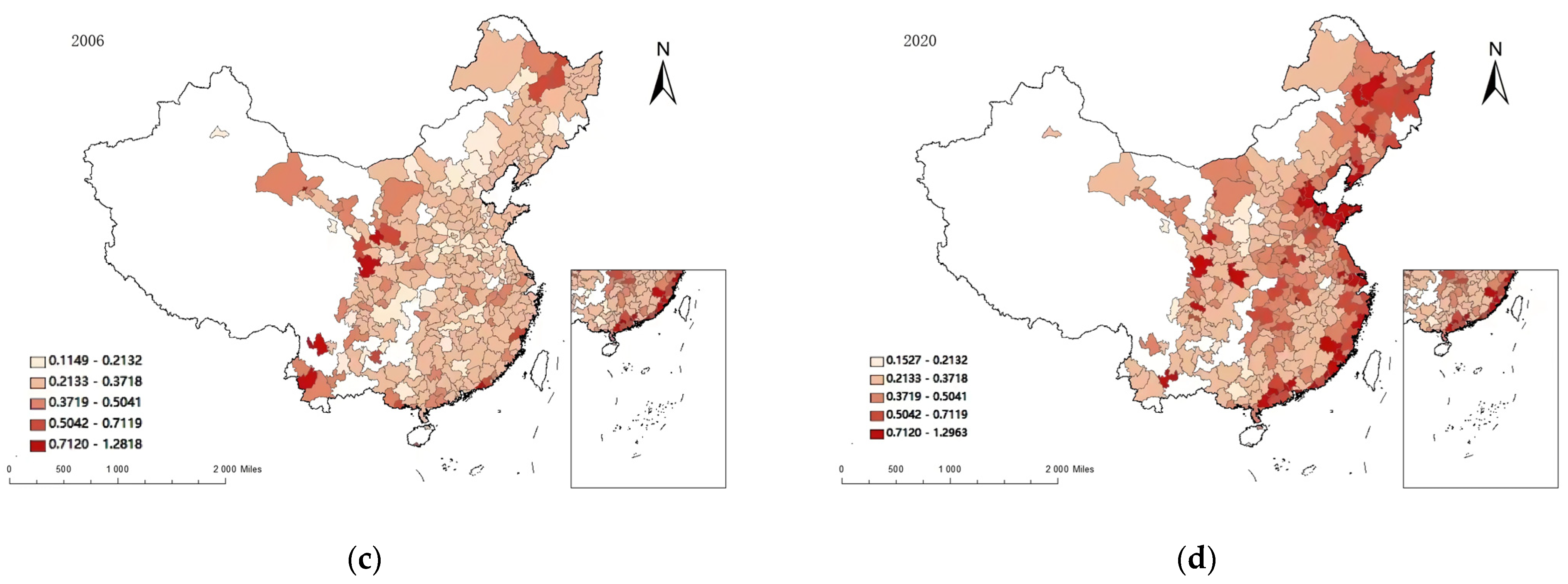
Using ArcGIS 10.4 software, we mapped the LRUE distribution in China for 2004, 2006, 2016, and 2020 (Figure 3). Based on the distribution of LRUE values, we classified them into five categories: low efficiency (≤0.6), medium-low efficiency (0.61–0.1–0.7), medium efficiency (0.71–0.8), medium-high efficiency (0.81–1.0), and high efficiency (>1.0). Previous studies focus more on evaluating land resource use efficiency without too much consideration of the relationship between economic agglomeration and LRUE. High use efficiency (LUE) in these agglomerations demonstrates that “the more intensive the city is, the higher is its use efficiency” [62]. However, our study presents different results after considering the ecological factors.
During the observation period, the distribution area of high efficiency changed: In 2004, the high-efficiency areas are mainly distributed in the northern region and a few are scattered around southwest regions. This was not due to the realization of an increased LRUE among these regions, but because of the underdeveloped economy, unexploited ecological environment, and relatively fair social distribution, so comprehensive efficiency is high because of a combination of low input and low undesired output. After 2006, the disadvantages caused by extensive development in these regions gradually appeared. Some cities have shifted from the high-efficiency areas, while a dramatic increase in the efficiency value among other cities is not observed. After 2016, the spatial distribution characteristics of “high in the east, low in the west” appear to be obvious, and the high efficiency values are gradually concentrated in the eastern and northeastern regions and provincial capitals of China. These regions have a decent economic foundation and pay more attention to the improvement of human capital accumulation and technical level, which leads to a continuous increase in the LRUE. The spatial spillover effect is one of the factors that affect the spatial and temporal evolution trend of LRUE. However, there are other reasons that LRUE is probably influenced by the policy implementation efficiency, economic foundation, technological conditions, and environmental awareness in the different regions. Moreover, high land prices force the cities in eastern regions to use land resources more effectively, and the urban built-up area there expanded rapidly.
5.3. Spatial Spillover Phenomenon
This subsection focuses on the spatial spillover phenomenon (direct and indirect effects) of LRUE, as shown in Table 5. The direct effect reflects the impact of economic agglomeration in the region on the LRUE, while the indirect effect reflects the impact of economic agglomeration in other regions (depending on the spatial weight matrix) on the LRUE of the region.
In terms of direct effects, economic agglomeration has a U-shaped relationship with LRUE; i.e., in the early stages of economic agglomeration, the crowding effect is greater than the agglomeration effect, making factors such as high pollution and inequitable distribution worsen LRUE. The economic agglomeration, after a long period of “agglomeration–diffusion–agglomeration”, optimizes the allocation of resources, improves regional knowledge and technology, and reduces distributional inequalities. This leads to a reduction in the undesired output of the LRUE, which in turn increases the LRUE.
In terms of indirect effects, there is still a U-shaped relationship between economic agglomeration and LRUE. In the early stages of economic agglomeration, the rapid transfer of economic activities to other regions reduces the production factors in the region, while the pollutants generated in other regions (especially in neighboring regions) will spread to the region, resulting in a reduction in its LRUE. However, when the economic agglomeration of other regions reaches a mature stage, it achieves the optimal allocation of resources and generates knowledge spillover effects. This helps the region to improve its LRUE level through exchange, cooperation, and learning by imitation.
5.4. Policy Recommendations
Based on the above findings, this paper makes the following recommendations:
- (1)
- Reasonably guide economic agglomeration and improve its scope and quality in order to contribute to positive externalities. The U-shaped relationship between economic agglomeration and LRUE shows the following: when the development level of economic agglomeration is low, externalities cannot be revealed; when economic agglomeration develops too fast, it generates a crowding effect, leading to a waste of resources and social injustice, making LRUE decrease; when economic agglomeration develops maturely, resources are fully utilized and LRUE improves. Therefore, the negative effects of economic agglomeration are temporary and can be avoided. Local governments should apply this law of development in a reasonable manner.
- (2)
- Mitigate the problem of over-agglomeration. Some regions in China have the problem of over-agglomeration, which is detrimental to the development of both the region and neighboring regions. Therefore, local governments should use policy tools to guide the level of agglomeration in a reasonable manner.
- (3)
- Develop an economic agglomeration strategy with local characteristics. Currently, China’s economic agglomeration and LRUE show great differences in spatial distribution, which implies that localities should tailor their economic agglomeration policies to guide high-quality economic agglomeration behavior according to their own strengths and weaknesses as well as the stage of agglomeration.
6. Conclusions
Based on the panel data of 281 prefecture-level cities in China from 2004 to 2020, this study explores the impact of economic agglomeration on LRUE by using the spatial lag model. After performing a series of tests, we obtained robust conclusions: (1) there is a positive spatial spillover effect on LRUE, and an increase in LRUE in the region helps to improve LRUE in neighboring regions; (2) there is a U-shaped relationship between economic agglomeration and LRUE.
There are still some shortcomings in this research due to the limits of time, energy, and length. First, the heterogeneity of economic agglomeration can be further discussed. As far as different regional economic developments are concerned, it is possible to discuss China’s eastern, central, and western regions separately. Secondly, in this study, we used prefecture-level city data; the sample size could be larger if county-level city data are used. Thirdly, the transmission mechanism of economic agglomeration and LRUE can be further studied.
Author Contributions
Conceptualization, N.Y. and Y.M.; methodology, N.Y.; formal analysis, N.Y. and Y.T.; data curation, N.Y.; writing—original draft preparation, N.Y.; writing—review and editing, Y.T. and Y.M.; supervision, Y.T. All authors have read and agreed to the published version of the manuscript.
Funding
This research was funded by the National Natural Science Foundation of China, grant number 71072066, the National Social Science Foundation of China, grant number 22BJY065, the Soft Science in Gansu Province, grant number 22JR4ZA060 and the Sichuan University, grant number 2019hhf-14.
Data Availability Statement
See text for access to all data.
Conflicts of Interest
The authors declare no conflict of interest.
| 1 | A prefecture-level city refers to a city that ranks below province and above county as an administrative division of China, which usually governs a couple of subordinated areas including some county-level cities. |
References
- Shu, C.; Xie, H.; Jiang, J.; Chen, Q. Is Urban Land Development Driven by Economic Development or Fiscal Revenue Stimuli in China? Land Use Policy 2018, 77, 107–115. [Google Scholar] [CrossRef]
- Lee, C.-C.; Wang, C.-S. Does natural resources matter for sustainable energy development in China: The role of technological progress. Resour. Policy 2022, 79, 103077. [Google Scholar] [CrossRef]
- Song, W.; Cao, S.; Du, M.; Lu, L. Distinctive roles of land-use efficiency in sustainable development goals: An investigation of trade-offs and synergies in China. J. Clean. Prod. 2023, 382, 134889. [Google Scholar] [CrossRef]
- Sueyoshi, T.; Yuan, Y. China’s regional sustainability and diversified resource allocation: DEA environmental assessment on economic development and air pollution. Energy Econ. 2015, 49, 239–256. [Google Scholar] [CrossRef]
- Shi, T.; Zhang, W.; Zhou, Q.; Wang, K. Industrial structure, urban governance and haze pollution: Spatiotemporal evidence from China. Sci. Total. Environ. 2020, 742, 139228. [Google Scholar] [CrossRef]
- Li, J.; Xu, C.; Chen, M.; Sun, W. Balanced development: Nature environment and economic and social power in China. J. Clean. Prod. 2018, 210, 181–189. [Google Scholar] [CrossRef]
- Li, Y.; Tang, Y.; Wang, K.; Zhao, Q. Environmental Regulation and China’s Regional Innovation Output—Empirical Research Based on Spatial Durbin Model. Sustainability 2019, 11, 5602. [Google Scholar] [CrossRef]
- Ge, T.; Li, C.; Li, J.; Hao, X. Does neighboring green development benefit or suffer from local economic growth targets? Evidence from China. Econ. Model. 2023, 120, 106149. [Google Scholar] [CrossRef]
- Wu, C.; Wei, Y.D.; Huang, X.; Chen, B. Economic transition, spatial development and urban land use efficiency in the Yangtze River Delta, China. Habitat Int. 2017, 63, 67–78. [Google Scholar] [CrossRef]
- Li, Q.; Wei, J.; Gao, W. Spatial differentiation and influencing factors of land eco-efficiency based on low carbon perspective: A case of 287 prefecture-level cities in China. Environ. Challenges 2023, 10, 100681. [Google Scholar] [CrossRef]
- Hong, W.; Wang, W.; Guo, R. Policies for optimizing land-use layouts in highly urbanized areas: An analysis framework based on construction land clearance. Habitat Int. 2022, 130, 102697. [Google Scholar] [CrossRef]
- KIJI, S. A study of the industrial area—Agglomeration of industries in an area. Geogr. Rev. Jpn. 1952, 25, 478–485. [Google Scholar] [CrossRef] [Green Version]
- Starrett, D. Market allocations of location choice in a model with free mobility. J. Econ. Theory 1978, 17, 21–37. [Google Scholar] [CrossRef]
- Schmutzler, A. The new economic geography. J. Econ. Surv. 1999, 13, 355–379. [Google Scholar] [CrossRef] [Green Version]
- Krugman, P. Increasing Returns and Economic Geography. J. Political Econ. 1991, 99, 483–499. [Google Scholar] [CrossRef]
- Head, K.; Mayer, T. Regional wage and employment responses to market potential in the EU. Reg. Sci. Urban Econ. 2006, 36, 573–594. [Google Scholar] [CrossRef] [Green Version]
- Feldman, M.P.; Audretsch, D.B. Innovation in cities: Science-based diversity, specialization and localized compe-tition. Eur. Econ. Rev. 1999, 43, 409–429. [Google Scholar] [CrossRef]
- Rosenthal, S.S.; Strange, W.C. The Determinants of Agglomeration. J. Urban Econ. 2001, 50, 191–229. [Google Scholar] [CrossRef] [Green Version]
- Konishi, H. Formation of Hub Cities: Transportation Cost Advantage and Population Agglomeration. J. Urban Econ. 2000, 48, 1–28. [Google Scholar] [CrossRef] [Green Version]
- Klaesson, J. Monopolistic competition, increasing returns, agglomeration, and transport costs. Ann. Reg. Sci. 2001, 35, 375–394. [Google Scholar] [CrossRef]
- Alfaro, L.; Chen, M.X. The global agglomeration of multinational firms. J. Int. Econ. 2014, 94, 263–276. [Google Scholar] [CrossRef] [Green Version]
- Jaffe, A.B.; Trajtenberg, M.; Henderson, R. Geographic Localization of Knowledge Spillovers as Evidenced by Patent Citations. Q. J. Econ. 1993, 108, 577–598. [Google Scholar] [CrossRef]
- Audretsch, D.B.; Feldman, M.P. R&d spillovers and the geography of innovation and production. Am. Econ. Rev. 1996, 86, 630–640. [Google Scholar] [CrossRef]
- Keeble, D.; Nachum, L. Why do business service firms cluster? Small consultancies, clustering and decentralization in London and southern England. Trans. Inst. Br. Geogr. 2002, 27, 67–90. [Google Scholar] [CrossRef]
- Knack, S.; Barro, R. Determinants of Economic Growth. South. Econ. J. 1998, 65, 185. [Google Scholar] [CrossRef]
- Feng, Y.; Lee, C.-C.; Peng, D. Does regional integration improve economic resilience? Evidence from urban agglomerations in China. Sustain. Cities Soc. 2023, 88, 104273. [Google Scholar] [CrossRef]
- Xu, H.; Wang, K.; Li, G.; Zhang, Y. How Officials’ Competitive Pressure Affects Sustainable Development Ca-pacity From a Spatial Perspective: Empirical Evidence From China. Front. Psychol. 2021, 12, 607232. [Google Scholar] [CrossRef]
- Kytzia, S.; Walz, A.; Wegmann, M. How can tourism use land more efficiently? A model-based approach to land-use efficiency for tourist destinations. Tour. Manag. 2011, 32, 629–640. [Google Scholar] [CrossRef]
- Zhu, X.; Li, Y.; Zhang, P.; Wei, Y.; Zheng, X.; Xie, L. Temporal–spatial characteristics of urban land use efficiency of China’s 35mega cities based on DEA: Decomposing technology and scale efficiency. Land Use Policy 2019, 88, 104083. [Google Scholar] [CrossRef]
- Zhang, X.; Jie, X.; Ning, S.; Wang, K.; Li, X. Coupling and coordinated development of urban land use economic efficiency and green manufacturing systems in the Chengdu-Chongqing Economic Circle. Sustain. Cities Soc. 2022, 85, 104012. [Google Scholar] [CrossRef]
- Liu, Y.; Sun, H.; Shi, L.; Wang, H.; Xiu, Z.; Qiu, X.; Chang, H.; Xie, Y.; Wang, Y.; Wang, C. Spatial-Temporal Changes and Driving Factors of Land-Use Eco-Efficiency Incorporating Ecosystem Services in China. Sustainability 2021, 13, 728. [Google Scholar] [CrossRef]
- Tian, Y.; Zhou, D.; Jiang, G. A new quality management system of admittance indicators to improve industrial land use efficiency in the Beijing−Tianjin−Hebei region. Land Use Policy 2021, 107, 105456. [Google Scholar] [CrossRef]
- Li, J.; Zhu, Y.; Liu, J.; Zhang, C.; Sang, X.; Zhong, Q. Parcel--level evaluation of urban land use efficiency based on multisource spatiotemporal data: A case study of Ningbo City, China. Trans. GIS 2021, 25, 2766–2790. [Google Scholar] [CrossRef]
- Zhao, Q.; Bao, H.X.; Zhang, Z. Off-farm employment and agricultural land use efficiency in China. Land Use Policy 2020, 101, 105097. [Google Scholar] [CrossRef]
- Burritt, R.; Schaltegger, S. Eco--efficiency in corporate budgeting. Environ. Manag. Health 2001, 12, 158–174. [Google Scholar] [CrossRef] [Green Version]
- Wang, X.; Zhang, Y.; Yu, D.; Qi, J.; Li, S. Investigating the spatiotemporal pattern of urban vibrancy and its determinants: Spatial big data analyses in Beijing, China. Land Use Policy 2022, 119, 106162. [Google Scholar] [CrossRef]
- Hosoe, M.; Naito, T. Trans-boundary pollution transmission and regional agglomeration effects*. Pap. Reg. Sci. 2006, 85, 99–120. [Google Scholar] [CrossRef]
- Solarek, K.; Kubasińska, M. Local Spatial Plans in Supporting Sustainable Water Resources Management: Case Study from Warsaw Agglomeration—Kampinos National Park Vicinity. Sustainability 2022, 14, 5766. [Google Scholar] [CrossRef]
- Ahmad, M.; Li, H.; Anser, M.K.; Rehman, A.; Fareed, Z.; Yan, Q.; Jabeen, G. Are the intensity of energy use, land agglomeration, CO2 emissions, and economic progress dynamically interlinked across development levels? Energy Environ. 2020, 32, 690–721. [Google Scholar] [CrossRef]
- Walter, I. The pollution content of American trade. Econ. Inq. 2010, 9, 61–70. [Google Scholar] [CrossRef]
- Copeland, B.R.; Taylor, M.S. North-South Trade and the Environment. Q. J. Econ. 1994, 109, 755–787. [Google Scholar] [CrossRef]
- Millimet, D.; Roy, J. Four New Empirical Tests of the Pollution Haven Hypothesis When Environmental Regulation is Endogenous; Tulane University: New Orleans, LA, USA, 2013. [Google Scholar]
- Wilson, J.D. Capital mobility and environmental standards: Is there a theoretical basis for a race to the bottom? Fair Trade Harmon. Prerequisites Free. Trade 1996, 1, 393–427. [Google Scholar]
- Cole, M.A.; Elliott, R. FDI and the Capital Intensity of “Dirty” Sectors: A Missing Piece of the Pollution Haven Puzzle. Rev. Dev. Econ. 2005, 9, 530–548. [Google Scholar] [CrossRef]
- Konisky, D.M. Regulatory Competition and Environmental Enforcement: Is There a Race to the Bottom? Am. J. Politi- Sci. 2007, 51, 853–872. [Google Scholar] [CrossRef]
- Lipscomb, M.; Mobarak, A.M. Decentralization and Pollution Spillovers: Evidence from the Re-drawing of County Borders in Brazil. Rev. Econ. Stud. 2016, 84, 464–502. [Google Scholar] [CrossRef] [Green Version]
- Kenworthy, J. The eco-city: Ten key transport and planning dimensions for sustainable city development. Environ. Urban. 2006, 18, 67–85. [Google Scholar] [CrossRef]
- Thissen, M.; Van Oort, F. European place—Based development policy and sustainable economic agglomeration. Tijdschr. Voor Econ. En Soc. Geogr. 2010, 101, 473–480. [Google Scholar] [CrossRef]
- Graham, D.J.; Kim, H.Y. An empirical analytical framework for agglomeration economies. Ann. Reg. Sci. 2007, 42, 267–289. [Google Scholar] [CrossRef]
- Combes, P.P.; Duranton, G.; Overman, H.G. Agglomeration and the adjustment of the spatial economys. Pap. Reg. Sci. 2005, 84, 311–349. [Google Scholar] [CrossRef]
- Acs, Z.J.; Audretsch, D.B.; Lehmann, E.E. The knowledge spillover theory of entrepreneurship. Small Bus. Econ. 2013, 41, 757–774. [Google Scholar] [CrossRef] [Green Version]
- Koster, S. Productive Places. The Influence of Technological Change and Relatedness on Agglomeration Externalities—By FRANK NEFFKE. Tijdschr. voor Econ. en Soc. Geogr. 2010, 101, 365–366. [Google Scholar] [CrossRef]
- Ke, S. Agglomeration, productivity, and spatial spillovers across Chinese cities. Ann. Reg. Sci. 2009, 45, 157–179. [Google Scholar] [CrossRef]
- Brülhart, M.; Mathys, N.A. Sectoral agglomeration economies in a panel of European regions. Reg. Sci. Urban Econ. 2008, 38, 348–362. [Google Scholar] [CrossRef] [Green Version]
- Moran, P.A.P. The Interpretation of Statistical Maps. J. R. Stat. Soc. Ser. B Methodol. 1948, 10, 243–251. [Google Scholar] [CrossRef]
- Pastor, J.T.; Lovell, C.A.K. A global Malmquist productivity index. Econ. Lett. 2005, 88, 266–271. [Google Scholar] [CrossRef]
- Lesage, J.; Pace, R.K. Introduction to Spatial Econometrics; Routledge: London, UK, 2008; pp. 19–44. [Google Scholar] [CrossRef]
- Elhorst, J. Matlab Software for Spatial Panels. Int. Reg. Sci. Rev. 2014, 37, 389–405. [Google Scholar] [CrossRef] [Green Version]
- Feng, Z.; Tang, Y.; Yang, Y. The relief degree of land surface in China and its correlation with population distribution. Acta Geogr. Sin. -Chin. Ed. 2007, 62, 1073. [Google Scholar] [CrossRef]
- Raupach, M.; Rayner, P.; Paget, M. Regional variations in spatial structure of nightlights, population density and fossil-fuel CO2 emissions. Energy Policy 2010, 38, 4756–4764. [Google Scholar] [CrossRef]
- Li, W.; Sun, B.; Zhao, J.; Zhang, T. Economic performance of spatial structure in Chinese prefecture regions: Evidence from night-time satellite imagery. Habitat Int. 2018, 76, 29–39. [Google Scholar] [CrossRef]
- Han, W.; Zhang, Y.; Cai, J.; Ma, E. Does Urban Industrial Agglomeration Lead to the Improvement of Land Use Efficiency in China? An Empirical Study from a Spatial Perspective. Sustainability 2019, 11, 986. [Google Scholar] [CrossRef] [Green Version]
Figure 1.
Influencing path of economic agglomeration on land resource use efficiency.
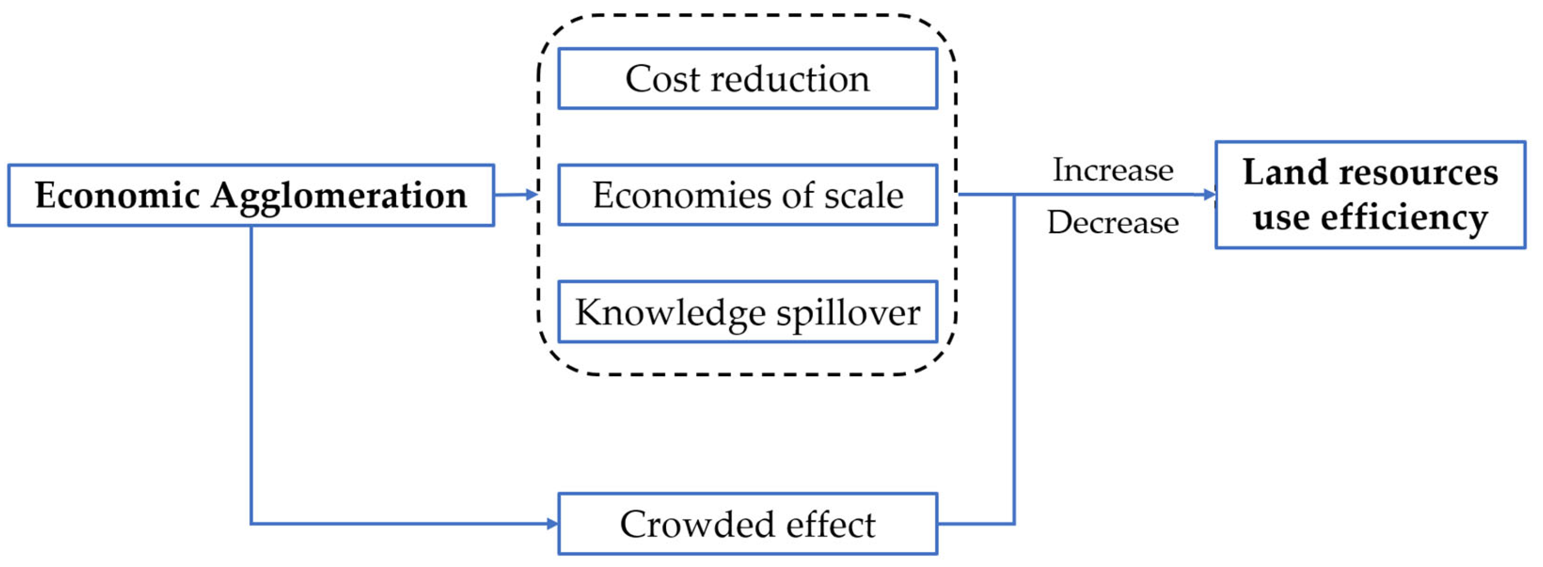
Figure 2.
Trends of land resource use efficiency by region in China from 2004 to 2020.

Figure 3.
Distribution of land resource use efficiency in 4 years: (a) land resource use efficiency in 2004; (b) land resource use efficiency in 2006; (c) land resource use efficiency in 2016; (d) land resource use efficiency in 2020.
Figure 3.
Distribution of land resource use efficiency in 4 years: (a) land resource use efficiency in 2004; (b) land resource use efficiency in 2006; (c) land resource use efficiency in 2016; (d) land resource use efficiency in 2020.


Table 1.
Description of all variables in the econometric model.
| Type | Full Name | Labels | Description |
|---|---|---|---|
| Explained variable * | Labor input | LRUE | Sum of the employment rate of the workplace and the self-employed individuals. |
| Capital input | Fixed capital stock calculated by perpetual inventory method. | ||
| Energy input | The annual electricity consumption. | ||
| Natural element input | Urban built-up area. | ||
| Expected output | Real GDP deflator based on 2003. | ||
| Undesired output | Environmental pollution (indicators of industrial waste); Social distribution (ratio of urban to rural disposable income); Social development opportunities (registered urban unemployment rate). | ||
| Explanatory variable | Economic agglomeration | Agg | Natural logarithm of non-agricultural output per unit area. |
| Square of economic agglomeration | Agg2 | The square term of Agg. | |
| Control variable | Production rate of labor | Lp | Natural logarithm of average labor output. |
| Degree of openness | Op | The total volume of import and export/GDP. | |
| Local industrial structure | Stru | The ratio of the secondary industry output value against the GDP. | |
| Environmental regulation | Rglt | Comprehensive utilization rate of industrial waste. | |
| Scientific and technological innovation level | Te | Civic expenditures on urban science and technology/GDP. |
* This variable is a composite indicator and is therefore represented by only one label.
Table 2.
Descriptive statistics of variables.
| Variable | Observations | Mean | STDEV | Min | Max |
|---|---|---|---|---|---|
| LRUE | 4777 | 0.3526 | 0.1809 | 0.0915 | 1.8263 |
| Agg | 4777 | 6.3964 | 1.4408 | 1.5439 | 11.3351 |
| Lp | 4777 | 3.0461 | 0.5633 | 1.0897 | 5.2671 |
| Op | 4777 | 0.1929 | 0.3142 | 0.0016 | 1.8364 |
| Stru | 4777 | 46.7327 | 11.0458 | 17.1000 | 73.8000 |
| Rglt | 4777 | 79.9185 | 21.9035 | 4.5400 | 100.0000 |
| Te | 4777 | 0.0109 | 0.0330 | 0.0000 | 0.2431 |
| Ups and Downs | 4777 | 0.6734 | 0.7557 | 0.0013 | 3.8138 |
| DN | 4777 | 0.8690 | 1.8967 | 0.0027 | 22.1829 |
Table 3.
Results of global Moran’s I test.
| Year | Land Resource Use Efficiency | Economic Agglomeration | ||
|---|---|---|---|---|
| Moran’s I | Z Statistics | Moran’s I | Z Statistics | |
| 2004 | 0.060 *** | 3.904 | 0.253 *** | 14.984 |
| 2005 | 0.094 *** | 6.004 | 0.254 *** | 14.991 |
| 2006 | 0.065 *** | 4.024 | 0.255 *** | 15.073 |
| 2007 | 0.076 *** | 4.634 | 0.257 *** | 15.202 |
| 2008 | 0.065 *** | 4.138 | 0.257 *** | 15.148 |
| 2009 | 0.061 *** | 3.851 | 0.254 *** | 14.975 |
| 2010 | 0.114 *** | 7.305 | 0.251 *** | 14.783 |
| 2011 | 0 112 *** | 7.092 | 0.244 *** | 14.371 |
| 2012 | 0.119 *** | 7.411 | 0.241 *** | 14.206 |
| 2013 | 0.108 *** | 6.953 | 0.245 *** | 14.410 |
| 2014 | 0.093 *** | 5.996 | 0.248 *** | 14.593 |
| 2015 | 0.083 *** | 5 249 | 0.250 *** | 14.670 |
| 2016 | 0.067 *** | 4.261 | 0.251 *** | 14.744 |
| 2017 | 0.123 *** | 7.689 | 0.254 *** | 14.911 |
| 2018 | 0.106 *** | 6.642 | 0.253 *** | 14.892 |
| 2019 | 0.103 *** | 6.331 | 0.251 *** | 14.781 |
| 2020 | 0 086 *** | 5.108 | 0.255 *** | 14.971 |
*** indicates statistical significance at the 1% level.
Table 4.
Regression results of the spatial econometric model.
| Explained Variable: LRUE | |||
|---|---|---|---|
| Adjacent Weight Matrix | Geographic Distance | Economic Distance | |
| Agg | −0.4629 *** (−18.82) | −0.2252 *** (−10.42) | −0.4997 *** (−20.45) |
| Agg2 | 0.0370 *** (29.03) | 0.0179 *** (15.33) | 0.0392 *** (30.90) |
| Lp | 0.1414 *** (17.03) | 0.0880 *** (12.31) | 0.1421 *** (16.99) |
| Op | 0.0110 (0.77) | 0.0036 (0.30) | 0.0068 (0.47) |
| Stru | −0.0003 (−0.87) | 0.0002 (0.66) | −0.0002 (−0.65) |
| Rglt | −0.0006 *** (−5.27) | −0.0003 *** (−2.65) | −0.0007 *** (−5.28) |
| Te | 0.0000 *** (2.65) | 0.0000 *** (3.12) | 0.0000 *** (2.92) |
| W*LRUE | 0.1555 *** (7.43) | 0.0523 *** (3.31) | 0.0657 * (1.92) |
| R-sq | 0.7075 | 0.7900 | 0.7034 |
* and *** indicate statistical significance at the 10% and 1% levels, respectively. Z statistics in parentheses.
Table 5.
Results of the effect decomposition of the spatial econometric model.
| Types | Variable | Explained Variable: LRUE | ||
|---|---|---|---|---|
| Adjacent Weight | Geographic Distance | Economic Distance | ||
| Direct effect | Agg | −0.4636 *** (−19.07) | −0.2253 *** (−10.23) | −0.4992 *** (−20.50) |
| Agg2 | 0.0371 *** (29.75) | 0.0180 *** (15.01) | 0.0391 *** (31.18) | |
| Control | YES | YES | YES | |
| Indirect effect | Agg | −0.0833 *** (−6.16) | −0.0122 *** (−3.14) | −0.0370 *** (−1.84) |
| Agg2 | 0.0067 *** (6.49) | 0.0010 *** (3.21) | 0.0029 *** (1.84) | |
| Control | YES | YES | YES | |
| Gross effect | Agg | −0.5469 *** (−18.40) | −0.2374 *** (−10.45) | −0.5361 ** (−17.36) |
| Agg2 | 0.0438 *** (28.75) | 0.0189 *** (15.58) | 0.0420 *** (23.16) | |
| Control | YES | YES | YES | |
** and *** indicate statistical significance at the 5% and 1% levels, respectively. Z statistics in parentheses.
Table 6.
A series of tests of the spatial econometric model.
| Test Object | Statistics | p-Value |
|---|---|---|
| LM rest no spatial | 34.1785 | 0.000 |
| Robust LM test no spatial lag | 27.2021 | 0.000 |
| LM test no spatial error | 16.0945 | 0.000 |
| Robust LM test no spatial error | 9.1181 | 0.003 |
| Hausman test | −99.6930 | 0.000 |
| LR-test joint significance spatial fixed effects | 4280.9887 | 0.000 |
| LR-test joint significance time-period fixed effects | 119.7880 | 0.000 |
Table 7.
Regression results of the spatial econometric model.
| Stage I | Stage II | ||
|---|---|---|---|
| Agg | Agg2 | LRUE | |
| Ups and Downs | −0.4139 *** (−20.78) | −4.612 *** (−21.41) | |
| DN | 0.2352 *** (18.85) | 4.0846 *** (21.77) | |
| Agg | −0.2715 *** (−8.95) | ||
| Agg2 | 03.022 *** (10.53) | ||
| Control variables | Yes | Yes | Yes |
| Constant items | −1.3372 *** (−5.66) | −51.0338 *** (−16.26) | 1.2915 *** (13.07) |
| F | 448.31 | 586.56 | |
| Adjusted R-sq | 0.7603 | 0.7986 | 0.2586 |
| Cragg–Donald Wald F statistic | 318.57 | ||
*** indicates statistical significance at the 1% level.
Disclaimer/Publisher’s Note: The statements, opinions and data contained in all publications are solely those of the individual author(s) and contributor(s) and not of MDPI and/or the editor(s). MDPI and/or the editor(s) disclaim responsibility for any injury to people or property resulting from any ideas, methods, instructions or products referred to in the content. |
© 2023 by the authors. Licensee MDPI, Basel, Switzerland. This article is an open access article distributed under the terms and conditions of the Creative Commons Attribution (CC BY) license (https://creativecommons.org/licenses/by/4.0/).
Share and Cite
MDPI and ACS Style
Yu, N.; Tang, Y.; Ma, Y. Spatio-Temporal Evolution, Spillover Effects of Land Resource Use Efficiency in Urban Built-Up Area: A Further Analysis Based on Economic Agglomeration. Land 2023, 12, 553. https://doi.org/10.3390/land12030553
AMA Style
Yu N, Tang Y, Ma Y. Spatio-Temporal Evolution, Spillover Effects of Land Resource Use Efficiency in Urban Built-Up Area: A Further Analysis Based on Economic Agglomeration. Land. 2023; 12(3):553. https://doi.org/10.3390/land12030553
Chicago/Turabian StyleYu, Naifu, Yingkai Tang, and Ying Ma. 2023. "Spatio-Temporal Evolution, Spillover Effects of Land Resource Use Efficiency in Urban Built-Up Area: A Further Analysis Based on Economic Agglomeration" Land 12, no. 3: 553. https://doi.org/10.3390/land12030553
Note that from the first issue of 2016, this journal uses article numbers instead of page numbers. See further details here.