Modelling Initiation Stage of Backward Erosion Piping through Analytical Models

Abstract

Backward erosion piping, which is one of the leading causes of levee and dam failures, is more likely to occur when a flow is concentrated on a defect with an overlying low-permeability layer and a shallow erosion channel forming and progressing towards a seepage source. Two analytical models are presented to allow assessment of the seepage regime on the initiation stage of BEP. The variations between the two models are analysed, indicating that the effects of soil loosening have a major role in the assessment of BEP mechanisms. This paper also describes the reliability of using Xiao’s model in 3D analysis, which includes results and parametric analysis. Although the head in front of the tip of the erosion channel can be predicted by this accepted calculation model, which is essential for laboratory work on this topic, the model also has range and boundary limitations that need to be addressed for general prediction when BEP progresses with channel development.

1. Introduction

One of the least understood mechanisms of internal erosion that accounts for a large percentage of dam and levee failures worldwide is backward erosion piping (BEP) [1,2], which is also dominant in natural landscapes and leads to linear erosion structures, named gullies [3]. BEP occurs when either an existing defect in the clay layer or a heave-induced crack undergoes a breakthrough, forming shallow erosion pipes that progress upstream by removing individual non-plastic soil particles from the defect, as illustrated in Figure 1. The BEP mechanism includes the following components: (1) the formation of a loosened zone around the blanket defect in the high-permeability layer, (2) detachment of individual soil particles into the low-permeability layer, (3) transportation of soil particles to the surface of the blanket defect (exit), and (4) formation of one or several pipes located between the interface of the low- and high-permeability layers. First, the loosened zone initially forms underneath the exit location, where the concentrated flow imposes increasing hydraulic gradients at the base of the defect. As the hydraulic gradient and flows increase, the increased flow velocity in the defect begins to carry soil particles to the ground surface in fluid suspension (i.e., a Stokes’s law phenomenon). With the removal of sand particles from the flow path, an erosion channel is formed, and the seepage flow from the surrounding soil tends to converge into the pipe. As the flow is increased, the pipe may propagate towards the flow source, forming one or several pipes that might eventually lead to the collapse of the foundation.

2. Literature Review

Tools for the prediction of piping have been developed since the early 1900s. Bligh [4,5] was the first to establish empirical formulae to determine the critical differential head based on specific cases of piping. Lane [6] adjusted the empirical formulae considering the weight factor by taking into account different types of embankment soils.

Numerous laboratory investigations have been conducted through flume tests to observe the BEP mechanisms and the critical hydraulic conditions needed to investigate the BEP process. A wide variety of BEP tests in various flume sizes have been performed to investigate the critical seepage conditions that influence BEP development beneath a structure [7,8,9,10,11,12] Most experiments have indicated that BEP initiation can be detected at one differential head, but then reaches an equilibrium state without a greater increase in the differential head, which is needed for the pipe to lengthen. However, in some of the experiments, the BEP can initiate at one differential head and then progresses backwards continuously towards the seepage source without reaching any equilibrium [13,14,15,16]. Schmertmann [17] found that the uniformity coefficient of the sand was significant in determining the erosion potential through a variety of experimental flumes that were used to analyse the critical heads needed for BEP initiation and progression. Chaplot [18] assessed the relationship between gully side-wall retreat over an entire year and selected factors of the environment, such as the terrain morphology, parent material, and soil types. Wilson [19] evaluated the propensity of soil pipe flow under constant head conditions to cause tunnel collapse and determined the effect of the initial soil pipe size on the ability to initiate pipe flow. Robbins [20] evaluated the progression rate of backward erosion through analyses of small-scale flume experiments to indicate the influence of the seepage velocity, particle diameter, and void ratio on pipe progression rate. While these flume experiments have typically focused on the behaviour of the BEP processes, their main purpose was to predict the critical hydraulic loading leading to BEP initiation and progression to failure. However, little consideration of the mechanisms concerning erosion initiation has been taken, although they actually play a significant role in understanding BEP development.

Several analytical predictive methods for determining the critical head have been developed to investigate the critical conditions that lead to BEP failure. Sellmeijer [21] combined groundwater flow equations with equations for the microscale processes in a pipe to simulate erosion, and Hoffmans [22] applied the Shields–Darcy model to predict pipe erosion. The Sellmeijer model was validated to perform good predictions for all laboratory scales with 2D configurations, but overpredicts the critical gradient in a 3D configuration [23] even after being recently adapted based on the results of additional experiments [24]. The Hoffmans model is used to calculate the critical hydraulic gradient under the condition that backward erosion leads to dike failure, but only a small percentage of BEP initiation cases can progress to failure conditions through field evidence [25,26]. For these reasons, assessing the hydraulic conditions related to the stages of BEP is of interest.

The existence of loosened zones has been observed in the laboratory and considered to be taken into account when determining a criterion of BEP [27,28,29,30] and field evidence of loosened zones has been observed in field deposits [31]. However, very little research has been conducted on detecting the progression of the loosened zone through direct observation and considering the soil loosening effects on analytical solutions that were developed to predict the critical head for BEP progression.

Previous experimental efforts were performed at two different scales with water exiting a circular hole in the cover layer [32]. The purpose was specifically to investigate channel tip features that are suitable for the analysis of the trend of the loosened zone. Figure 2 presents observations from one of the tests deflecting the vertical section of the tip of the channel. With increasing hydraulic gradient across the sample, the channel eventually initiates and develops over a certain distance, channel equilibrium is then observed, and the gradient needs to be raised again until the channel progressed in the upstream direction, as seen in Figure 2a. However, the channel absolutely progresses to the seepage source for the entire process, as seen in most experiments, but also with a downwards process within development. Fleshman [27] found that the loosened zone increases in thickness with increasing gradient across the sample through vertical-flow experiments. Additional increases in the gradient reduce the downwards force of the upper grains on the next layer of the underlying grains, allowing them to loosen until they have reached critical movement conditions, at which point loosened soil particles are removed from the channel, as shown in Figure 2b. The progression of the tip of the channel acts like a resistance wall: the soil mass at the back of the tip of the channel causes failure, while the soil mass for resisting failure at the front of the channel is removed. The soil mass is eventually observed to collapse into the channel when reaching critical conditions, and then the soil is transported through the channel and out of the exit while the channel develops towards the upstream side.

Although the model had been validated through experiments [33], application has typically been limited to 2D analysis (3D configuration with 10 mm width only and without investigation of multiple channels around the exit area). The limited evidence has resulted in the equations being assessed over a very narrow range of seepage configurations, potentially limiting the generality of the analysis of BEP mechanisms. In the present study, Xiao’s model is compared to Wu’s model, which is widely used in China to calculate the seepage field with a downstream exit, to allow for evaluation of the practical use for general prediction.

The more common application of this model is presented in this paper (i.e., initial stage of backward erosion piping and three-dimensional analysis of Xiao’s model). Wu’s model, which satisfies most analyses, has been widely used in China for decades and has been proven to predict the head distribution around the edge of a defect or ditch. Therefore, in the present study, Wu’s model is used to compare with Xiao’s model in order to validate the prediction capability of the latter, followed by analysis of the effects leading to variations through comparison between these two analytical solutions. In addition, this paper also presents the reliability of using Xiao’s model in 3D analysis. The numerical results are compared to laboratory results to validate its practical use for simulation, and parametric studies are performed to provide a better understanding of the erosion mechanism of BEP.

3. Comparison between the Two Analytical Models

To calculate the critical gradient at the tip of the channel that causes channel development, numerical models can be refined to deliver output very near the singularity, but this always results in an averaged value for the exit gradient rather than an exact value. The numerical analysis is therefore combined with an exact solution that is likely to be valid near the singularity. The exact solution for groundwater flow near the exit hole can be determined by using conformal analysis of Xiao’s or Wu’s model.

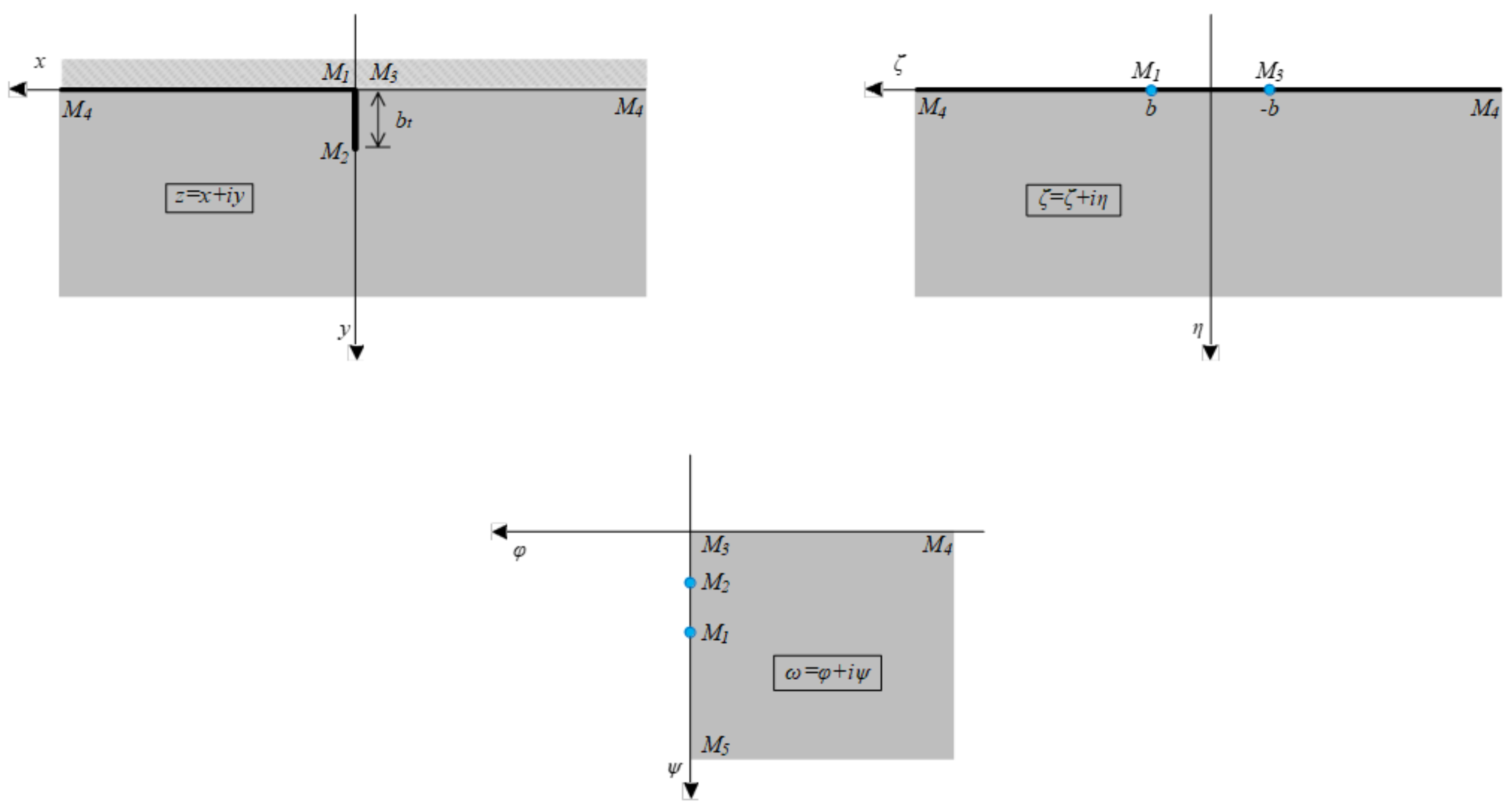
3.1. Xiao’s Model [33]

The exact solution for groundwater flow near the pipe tip in Xiao’s model is determined using conformal analysis. The complex potential ω (ω = Φ + iΨ = −KH + iΨ, in which Φ is the groundwater potential, K is the permeability, H is the groundwater head, and Ψ is the stream function as a function of the complex coordinate z (z = x + iy)) can be obtained for this configuration (Figure 3). This mapping can be fulfilled using Equation (1):

$$\omega =iT\sqrt{b+\sqrt{z^2+b^2}}$$

(1)

where b represents the depth of the ditch and T is a constant. When $\mathrm{Im}\sqrt{z^2+b^2}=0$ $\mathrm{Im}\sqrt{z^2+b^2}=0$ and Re(z) < 0, the minus sign is used in Equation (1) other cases, the plus sign is used.

Equation (2) can also be written into the form of z expressed in terms of ω:

$$z=\pm \sqrt{{\left[{\left(\frac{\omega }{T}\right)}^2+b\right]}^2-b^2}$$

(2)

where the positive and negative sign selections are the same as those in Equation (1)

The constant T can be obtained by substituting the head (H₀) at one point (z = x₀ + iy₀) outside the ditch in Equation (3)

$$T=\frac{K{H}_0}{\mathrm{Im}\sqrt{b\pm \sqrt{{\left(x_0+i{y}_0\right)}^2+b^2}}}$$

(3)

where the selection of positive and negative signs is the same as Equation (1) Substituting y₀ = 0 and x₀ < 0 (a point on the top of the sand layer in front of the pipe tip) in Equation (4) T can be presented by:

$$T=\frac{K{H}_{\mathrm{o}}}{\mathrm{Im}\sqrt{b-\sqrt{x_{\mathrm{o}}{}^2+b^2}}}=\frac{K{H}_{\mathrm{o}}}{\sqrt{\sqrt{x_{\mathrm{o}}{}^2+b^2}-b}} (x_0 < 0)$$

(4)

where the selection of positive and negative signs is the same as Equation (1)

If b = 0, then $\mathrm{Im}\sqrt{z^2}>0$; taking the positive sign, Equations (2) and (4) can be rewritten as:

$$z={\left(\frac{\omega }{B}\right)}^2\hspace{1em}B=\frac{k{H}_0}{\sqrt{\left|x_0\right|}}\hspace{1em}(x_0<0)$$

(5)

yields:

$$z={\left(\frac{\omega }{k{H}_0}\right)}^2\left|x_0\right|\hspace{1em}\omega =-k{H}_0\sqrt{\frac{z}{\left|x_0\right|}}$$

(6)

Equation (6) represents the seepage solution for pipe erosion, for which the following remarks can be made: the constant number B can be calculated when the head at a certain point (H₀) within the seepage field is known; then, the head at any position around this seepage field can be assessed by substituting the point coordinates.

3.2. Wu’s Model [34]

As Xiao’s model presented here involves head distributions in BEP development, including sand boiling and channel progression, it can be used as a basis for comparison with models predicting the seepage field around the exit at the point before channel initiation, such as Wu’s model.

The Wu model is implemented in a 3D numerical groundwater model referred to as an infinity swallow ditch (with width but without depth) with infinite depth of permeable sand layer to account for different diameters of seepage exit and used to derive a solution using Forchheimer equations for predicting the seepage field located on the exit area of a homogeneous confined aquifer. The model has been verified by comparison with many experiments and finite element results in China [35,36].

For the condition of a permeable layer with infinite thickness, the deviation of the flow net around shallow ditches can be composed of two sets of conjugate orthogonal loops, including the ellipsoidal surface and the hyperboloid of revolution, as shown in Figure 4. Considering that the width of the exit is equal to 2b₁ and the midpoint of the exit is the origin of the coordinates within the control of unit discharge q, the coordinates can be obtained by the groundwater potential and the stream function as follows:

$$\left\{\begin{array}{c}x=b_1\cos \tilde{\psi }\mathrm{ch}\tilde{\phi }\\ y=b_1\sin \tilde{\psi }\mathrm{sh}\tilde{\phi }\end{array}\right.\hspace{1em}\hspace{1em}\tilde{\phi }=\frac{\pi \phi }{q}\hspace{1em}\tilde{\psi }=\frac{\pi \psi }{q}$$

(7)

where φ represents the potential function, ψ is the stream function, and q is the unit discharge.

The complex coordinate z (z = x + iy)) can be described as:

$$z=x+iy=b_1\cos \frac{\pi \psi }{q}\mathrm{ch}\frac{\pi \phi }{q}+i{b}_1\sin \frac{\pi \psi }{q}\mathrm{sh}\frac{\pi \phi }{q}=b_1\mathrm{ch}\left(\frac{\pi }{q}\left(\phi +i\psi \right)\right)$$

(8)

Using Equation (9) by filling the complex potential ω (ω = Φ + iΨ = –KH + iΨ, where K is the permeability and H is the groundwater head),

$$z=b_1\mathrm{ch}\left(\frac{\pi }{q}\omega \right)$$

(9)

After resetting the origin of the coordinates to the left side of the edge of the exit, Equation (10). can be written as:

$$z_1=b_1\mathrm{ch}\left(\frac{\pi }{q}\omega \right)-b_1\hspace{1em}\frac{\pi }{q}\omega ={\mathrm{ch}}^{-1}\left(1+\frac{z_1}{b_1}\right)$$

(10)

As the constant head of point A at the top of the sand layer (z₁ = x₁₀) is equal to H₀, the value of the complex coordinate can be written as in Equation (11) after filling the complex potential with the known groundwater potential (φ = −kH₀):

$$x_{10}=b_1\mathrm{ch}\left(-\frac{\pi }{q}k{H}_0\right)-b_1\hspace{1em}-\frac{\pi }{q}k{H}_0={\mathrm{ch}}^{-1}\left(1+\frac{x_{10}}{b_1}\right)$$

(11)

Combining Equations (10) and (11) yields:

$$-\frac{\omega }{k{H}_0}=\frac{{\mathrm{ch}}^{-1}\left(1+\frac{z_1}{b_1}\right)}{{\mathrm{ch}}^{-1}\left(1+\frac{x_{10}}{b_1}\right)}=\frac{\ln \left(1+\frac{z_1}{b_1}\pm \sqrt{{\left(1+\frac{z_1}{b_1}\right)}^2-1}\right)}{\ln \left(1+\frac{x_{10}}{b_1}\pm \sqrt{{\left(1+\frac{x_{10}}{b_1}\right)}^2-1}\right)}$$

(12)

It is easy to conclude that not only is the absolute value of the ratio between the complex coordinate (z₁) and the half width (b₁) very small but also the value of the ratio between the complex coordinate at point A (x₁₀) and the half width (b₁) is very small if located near the exit. Then, Equation (13) can be obtained by assuming that the half width is close to infinity:

$$-\frac{\omega }{k{H}_0}\approx \frac{\ln \left(1\pm \sqrt{2\frac{z_1}{b_1}}\right)}{\ln \left(1\pm \sqrt{2\frac{x_{10}}{b_1}}\right)}\approx \frac{\sqrt{2\frac{z_1}{b_1}}}{\sqrt{2\frac{x_{10}}{b_1}}}=\sqrt{\frac{z_1}{x_{10}}}$$

(13)

yielding

$$z_1={\left(\frac{\omega }{k{H}_0}\right)}^2{x}_{10}\hspace{1em}\omega =-k{H}_0\sqrt{\frac{z_1}{x_{10}}}$$

(14)

As the positive direction of the x-coordinate in these two models is opposite, the calculated seepage field from these two models is identical if the depth of the ditch is equal to 0 through comparison of Equations (6) and (14).

3.3. Comparison of Models with Different Ditch Widths

As described above, the models are in good agreement within the condition of the half width of the ditch that can be taken into account, approaching infinity if the calculated point is located very close to the edge of the exit (the value of the ratio between the complex coordinate (z₁) and the half width (b₁) is very small, as the depth of the ditch is equal to 0). However, the erosion mechanism that causes the processes of BEP development might be related to the exact size of the ditch width and the head distribution calculated using Wu’s model, especially which is directly connected with its half width. It is therefore essential to compare hydraulic conditions with different ditch widths between these two models. If it is assumed that a point in the seepage field is located close to the edge of the exit (and thus close to the singularity) with the initial reference head, the calculated head at the distance from the edge of the exit can be assessed with these two models separately. As the deviations between these two models significantly increase as the distance increases, a maximum difference of 20% from the initial reference value is taken as a likely effective range for these two models to achieve accessible conversion. The relationship between the half ditch width and the range can be seen in Figure 5. To evaluate the distance to the edge of the exit that causes differential to the calculated head between these two models, a comparison between the distance to the edge of the exit and constant half ditch width is presented in Figure 6.

By regression analysis of the observed variations in Figure 5, the range is found to increase linearly with the size of the half width, and a linear equation describing the expected behaviour is deduced. However, as seen in Figure 6, the differential between the calculated results of the models increases rapidly while the distance to the edge of the exit increases; therefore, it is more likely that the distance plays a major role in causing the discrepancies between models, although increasing the half width can achieve better agreements within the calculated results.

4. Reliability in 3D Analysis

As illustrated in the literature review section, Xiao’s model is validated through experiments in 2D analysis [33]. The reliability of using the model in 3D analysis is presented here.

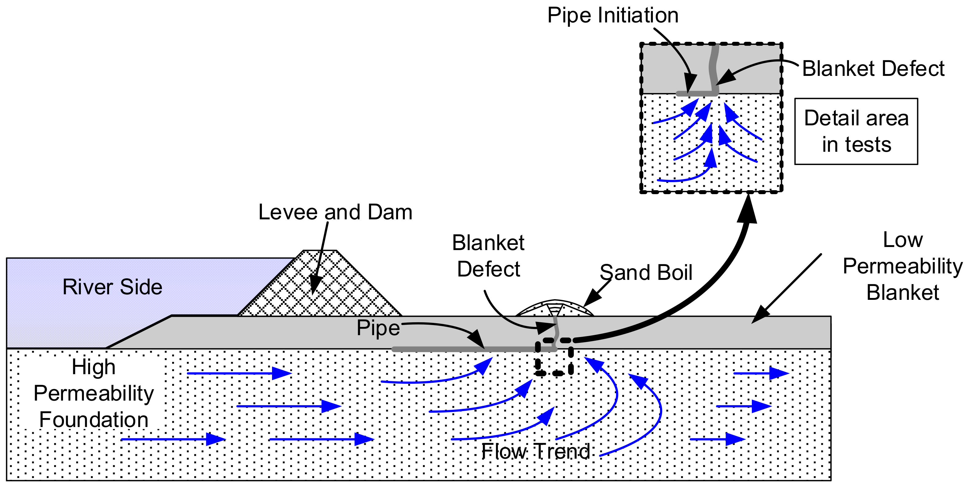
4.1. Physical Conditions in the Field

Figure 7a illustrates the condition that leads to initiation whereby flow is concentrated into the defect. The first phase of BEP initiation is illustrated in Figure 7b as loosening of the soil surrounding the exit and heaving of the soil into the open void. As the hydraulic gradient increases, the flow velocity in the defect becomes great enough to remove and carry soil particles in suspension (Figure 7c), the soil is “fluidized”, and eroded particles are transported to the surface, where they are deposited in a sand boil. With a further increase in the hydraulic gradient, the vertical dimension of the narrow ditch (the core of Xiao’s model) grows by progressing deeper, and then more particles loosen to maintain vertical equilibrium (Figure 7d). As the horizontal seepage force acting on the soil particles of the ditch increases rapidly, the surrounding particles move into the ditch, forming a BEP channel (Figure 7e). After the channel is formed, the erosion progression is mainly focused on channel development until equilibrium is achieved. Then, further progression can be treated as a repeated process between Figure 7d,e until total failure occurs.

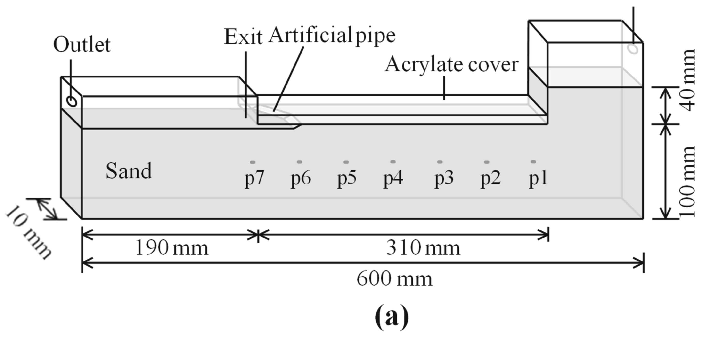
4.2. Adapted Conditions for the Laboratory Model

Experiments with an exit hole [32] simulated the case where a confining upper layer is locally punctured such that flow from the aquifer concentrates towards one point. The experimental work provides valuable information about the progression trend of the tip of the channel on the critical head.

The first observation to be made from Figure 8a,c is that channel equilibrium is observed, and the head needs to be raised until the channel length develops towards the upstream direction (opposite to the flow direction). As seen in Figure 8a,c, the tip of the channel appears to be a semicircular area. After the water head increases to exceed the critical condition, several soil particles are fluidized and washed away with seepage water on the downstream soil surface or running water surface, as seen in the red dashed ellipse area in Figure 8b,d. As seen in Figure 8b, the progression of the tip concentrates on the right side of its semicircle (the particle was eroded into a small ditch), while the progression in Figure 8d is more likely in the left and right sides at the same period.

Analysis of the area of channel lengthening in the experiments shows that the tip area before progression appears to be a semicircle where the pipe develops in a random alignment point of large interstitial voids in the loosening soil mass with preferential low resistance. Considering any potential point starting progression from the tip of the channel, it is clear that the distance from the centre of the semicircle is identical. The 3D general model can therefore be simplified to a 2D number of input parameters in the response surface. This model can either assume a semicircle area to calculate the three-dimensional seepage field to predict channel progression for the overall analysis or be simplified to a two-dimensional model with the centre of the semicircle as the origin point and a distance of r₀ for the analysis of channel development around the tip area, as seen in Figure 9.

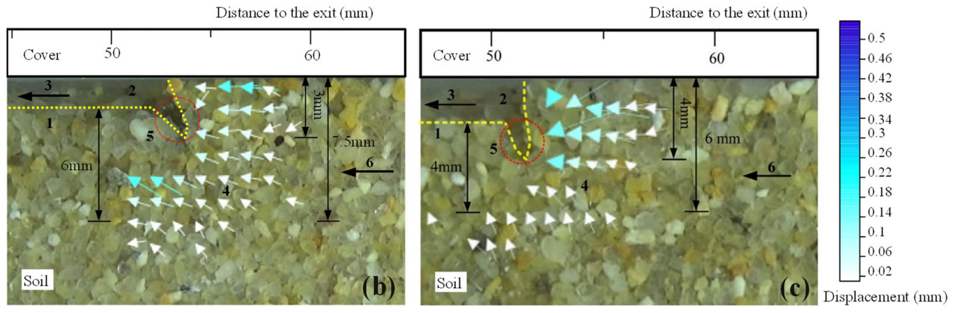
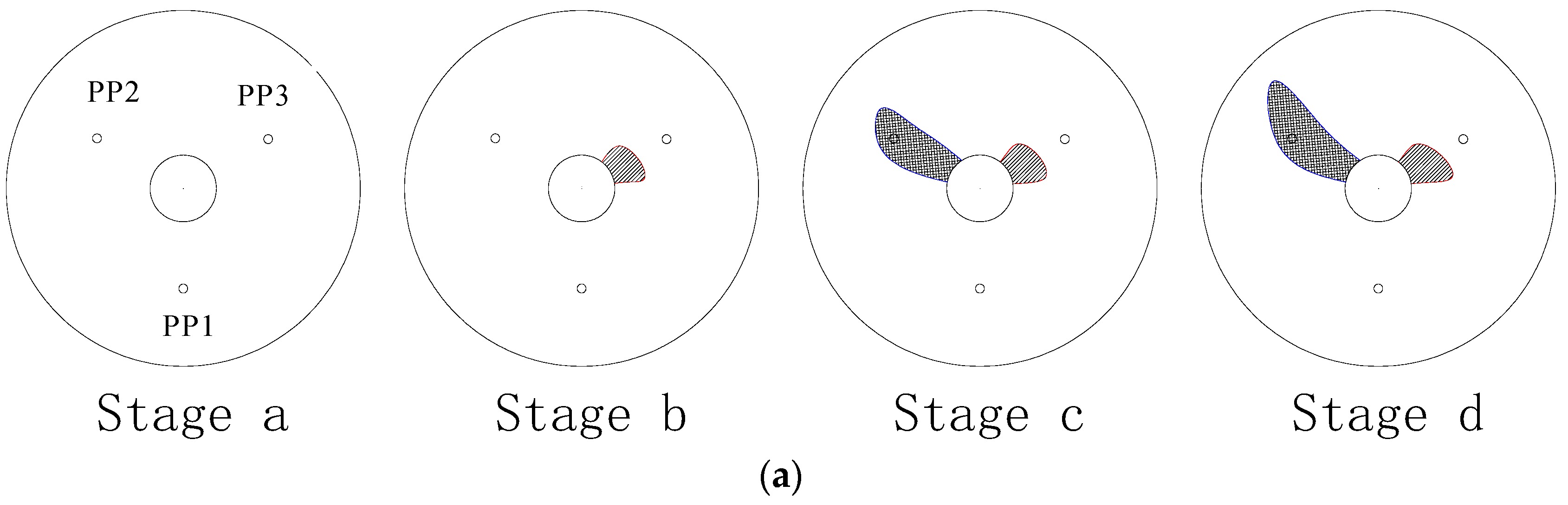
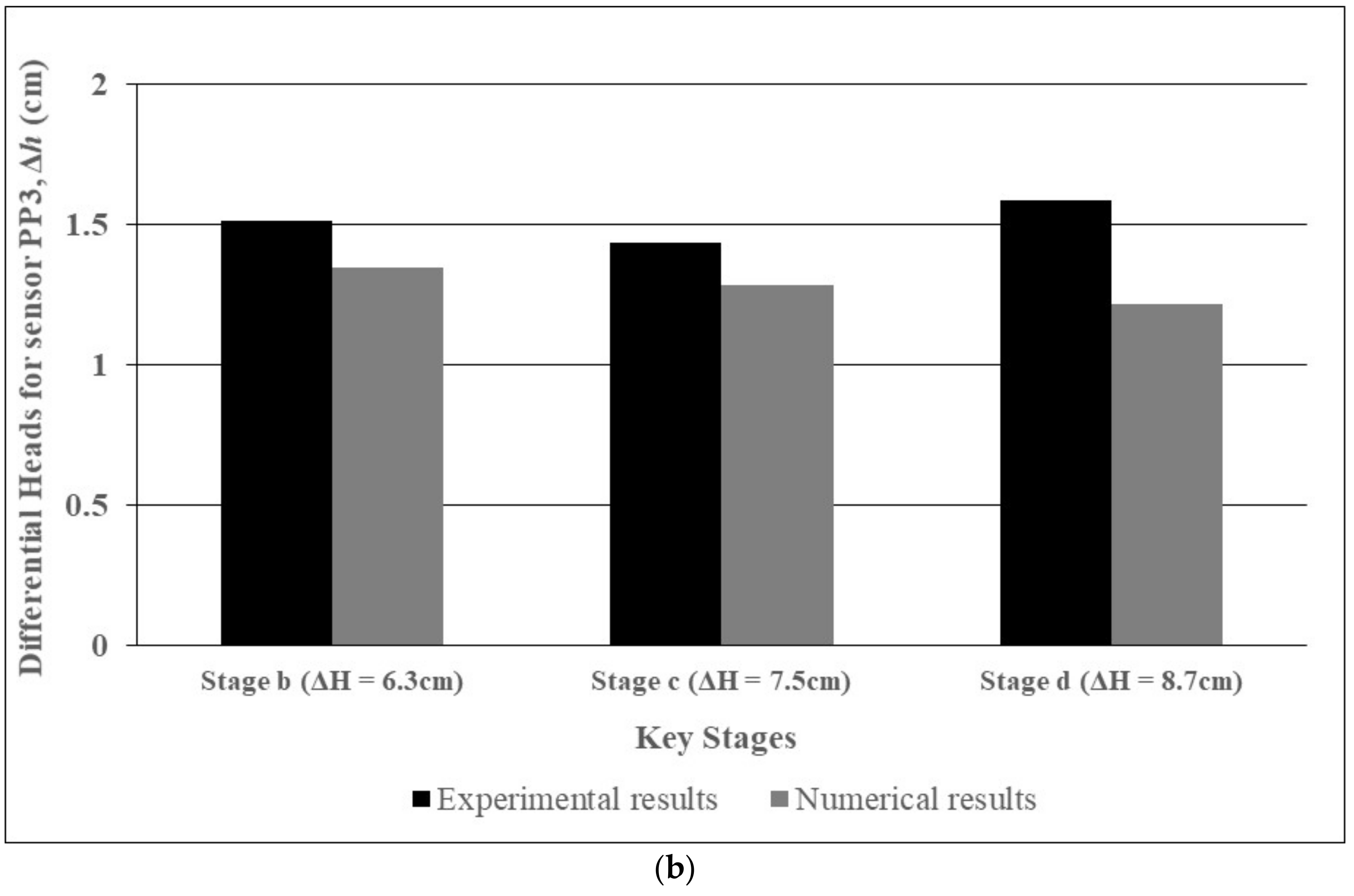
4.3. Results Analysis

An inverse analysis was previously developed to interpret the results in a series of 3D contour plots that represent the hydraulic head regime at each stage of BEP development [37] A stage with a total differential head equal to 7.6 cm is presented in Figure 10, which illustrates an example of potential channel development in 3D sand samples. The circular exit hole can be taken into account in the tip area before channel initiation. As seen in Figure 10, the channel could initiate at any point around the edge of the exit hole where the flow concentrates. For this condition, the edge of the exit hole in 3D configurations can be assumed to be the channel tip in 2D configurations, which is illustrated in Figure 10. The analysis can therefore be simplified to a two-dimensional analysis by establishing the straight corresponding line between the centre of the exit and the potential channel initiation point on the edge of the exit as the tip area, such as the line between PP2, PP3, A or B and the centre O.

As the model is presented to be used in 3D analysis, comparisons are made to assess how well the analytical model result correlated with actual laboratory results. Figure 11 presents a comparison of the experimental and numerical results by Xiao’s model of three key stages (stages b, c and d with total differential heads of 6.3, 7.5 and 8.7 cm, respectively) for sensor PP3. As the channels further develop, the differential head of sensor PP3 decreases, and the head calculated using the model decreases. Theoretically, the differential head of a sensor should decrease dramatically when a channel is formed in front or nearby, but the surrounding loosened zone occupies a proportional seepage concentration that slows down the sensor’s reaction regarding decreasing its differential head. However, it is important to acknowledge the loosened zone that exists in the physical models that is not considered in the analytical assumptions, as the effect of any loosened zone exists in real conditions, and the deviations are prominent.

Greater variations occur in the later test stages (stage d > stage c > stage b), as seen from Figure 11b, and these are likely due to differential loosening that may have occurred without being observable and formed in front of or below the channel when the channel progresses to a closer range to the sensor. Furthermore, the maximum deviation generally comes from the influence of other channels simultaneously forming in the experiments (another channel is initiated and develops towards sensor PP2 in Figure 11a). More seepage is concentrated in another channel in front of sensor PP2, which may lead to extra deflection of sensor PP3′s reaction to channel development, increasing the deviation between the numerical and laboratory results. In addition, a portion of the observed error can also be attributed to the distance while the channel tip is approaching the sensor, which causes the calculated head to be even lower. Although the results of the numerical model present lower values than the experimental results due to such reasons, it can be seen from Figure 11 that all stages achieved very close agreement between the experimental and numerical results; thus, the application of the model in three-dimensional analysis is still persuasive.

4.4. Parametric Analysis

As described in Xiao’s model [33] the critical condition for channel development is when the depth of the ditch in front of the channel tip continues to develop without reaching equilibrium. Then, the ditch soil collapses into the channel due to the horizontal seepage force, and the channel length is increased. Therefore, the assessment of the progression level can be determined by whether the critical value of the soil to maintain the equilibrium located in front of the channel tip is exceeded. As the seepage conditions near the channel tip can be determined, the soil particles in front of the tip can be divided into multiple unit widths of soil strips for the assessment. We consider the forces acting on any soil strip in Figure 12, which depicts the soil strip in front of the channel when a constant hydraulic gradient is imposed on the sample.

Considering the vertical force–balance analysis of the soil strips, the strip pushes the cover upwards when the vertical seepage force f_y acting on the strip is greater than its effective gravity G’, causing the test cell cover to provide counterforce to the soil. However, the upwards force acting on the cover is much less than its resistance to bending and deformation, and therefore the strip reaches a state of equilibrium in the vertical direction.

As equilibrium is achieved in the vertical direction and the upwards force of the soil strip continuously increases, the horizontal force f_x acting on the soil strip can be assessed. Within the horizontal seepage force acting on the soil strip, a frictional force f caused by the contact between the soil strip and the cover plate is initiated. The force can be calculated based on the frictional coefficient of the cover multiplied by its resistance force (f_y − G’) to maintain vertical equilibrium. No equilibrium can be observed in the horizontal direction for the soil strip when the horizontal seepage force f_x exceeds the frictional force f, and then the soil strip collapses and falls into the ditch, leading to channel progression until equilibrium is achieved or total failure occurs.

In summary, the channel progresses backwards to the seepage source only when any soil strip in front of the channel tip is subjected to not only a vertical upwards seepage force that is greater than its effective gravity but also a horizontal seepage force that is greater than its frictional force, or the process of progressively reaching equilibrium can be achieved and maintained.

Analyses of parameters. As described earlier, the mechanics of the BEP erosion process can be explained as the soil structure reacting to the increasing hydraulic gradient and flow by adjusting its structure with a zone of decreased density (sand boils) in conjunction with preferred seepage channels. These mechanisms are examined by considering the interaction of the various forces acting on the soil grains as the soil structure reacts to the increasing hydraulic gradient. To obtain a rational assessment of forces, the leading parameters are defined based on specific details of the values, which have significant impacts on erosion resistance.

Upwards force. Assuming the constant T can be calculated with known the head (H₀) at a point (z = x₀+iy₀) outside the ditch, the hydraulic gradient J (J = J_x − iJ_y, in which J_x and J_y are the horizontal and vertical components of the hydraulic gradient, respectively) can be obtained by taking the derivative of the complex potential x with respect to z on the basis of Equation (1) and the complex potential ω (ω = Φ + iΨ = −KH + iΨ, as described above),

$$J_x-i{J}_y=\frac{1}{K}\frac{d\omega }{dz}=i\frac{H_0}{\sqrt{\sqrt{x_0{}^2+b^2}-b}}\frac{z}{2\sqrt{b\pm \sqrt{z^2+b^2}}\left(\pm \sqrt{z^2+b^2}\right)}$$

(15)

where the selection of positive and negative signs is the same as in Equation (1). For any soil strip with height y_s, the upwards force P on top of the soil strip can be obtained by using Equation (11):

$$P=f_y-G^{\prime }={\gamma }_w{\displaystyle {\int }_0^{y_s}{J}_{y}dy-}{\gamma }^{\prime }{y}_s$$

(16)

where γ_w is the unit weight of water and γ’ is the buoyant unit weight of the soil.

As the value for y_s increases when the soil strip maintains a constant x-coordinate, the calculated value for J_y decreases, as seen by entering the coordinates into Equation (15), and the integrated results for Equation (16) establish an increasing trend until reaching the maximum. Therefore, the soil strip is assumed to start with one single grain and by successively increasing the number of grains until the maximum upwards force P_max and the numbers of particles for the soil strip are achieved, for which the maximum ditch depth is calculated, corresponding to the coordinates or stripe position to be selected. As the grain size varies in the sample even for uniform soil, the average grain size d₅₀ is taken into account to represent a single grain to simplify the assessment.

Interface frictional coefficient. The upwards force acting on the cover layer causes its counterforce to maintain balance. This effect acts similarly to the lateral earth pressures on a vertical wall that retains a soil mass. The cover layer can be assumed to be a resistance wall, while the soil stripes are assumed to be backfills. At this moment, the contact between the cover layer and the soil stripes is parallel, indicating that the coefficient of both inclined angles of the wall face to the vertical direction and the sloping angle of backfill are equal to zero. Thus, the interface frictional coefficient (δ) between the cover layer and soil samples depends on the internal friction angle of the soil (φ), for which typical values range from φ/2 to φ, with 2φ/3 most commonly used based on Coulomb’s earth pressure theory.

Horizontal seepage force. The horizontal seepage force is determined with the horizontal gradients acting on the tip of the channel and the ditch width. Experiments from others [32] indicated that the measurement of ditch depth is approximately three times the average grain size. Therefore, the depth can be substituted as the y-coordinate into Equation (10) to back-calculate the horizontal gradients J_x across the ditch area. However, it should be noted that the model considers the effects of the soil loosening around the ditch leading to channel development but does not take into account the soil loosening in front of the channel tip, which results in the predicted horizontal force being overestimated. In reality, soil loosening increases the hydraulic conductivity of the soil surrounding the preferential pathway in front of the tip area and significantly reduces the horizontal gradients of this area.

As derived from previous work from others [30] the hydraulic conductivity of the loosened zone is in the range of 3.5 to 6 times, and the flow was constant. Then, the actual horizontal gradient, i_a, can be calculated as the reciprocal of is ratio between the loosened zone and the base soil. Therefore, the horizontal seepage force f_x can be obtained by using Equation (17):

$$f_x={\gamma }_w{\displaystyle {\int }_0^{3d_{50}}{i}_a{J}_{x}dy}$$

(17)

where the range of i_a is between 0.165 and 0.285.

While the value of maximum upwards force P_max is determined on the basis of both soil strip heights (y_s) and vertical gradients (J_y), the frictional force (f) acting on soils caused by contact with the cover plate can be defined as the product result of the pressure force (P_max) and tangent of the frictional coefficient (tanδ). Therefore, the channel propagates with no extension of the length and reaches the state of equilibrium only if the frictional force (f) is not less than the value of the horizontal seepage force (f_x). Otherwise, the channel continues to grow until failure.

5. Discussion

The findings illustrate that the calculated results from the two models show good agreement within a small range around the exit area. However, the variations increase dramatically as the range increases. To find a possible explanation for the observed variations, the mechanisms of soil particles around the exit were analysed in detail. Wu’s model neglects the process of soil loosening and does not establish a clear trend with respect to changing permeability around the exit area, since the loosening of grains around the exit area may need to be taken into account when calculating the seepage field of this kind. Xiao’s model not only provides equations based on considerable soil loosening but also reveals that the existence of swallow ditches leading to soil collapsing causes channel initiation. Flow through the exit causes the effective hydraulic conductivity to increase due to the reduced density of the fluidized mass (fewer particles in suspension), leading to lateral soil boiling and even channel progression, which is the main evidence underlying this conclusion. In the seepage field calculation, the error magnitudes from the models are relatively small around the exit area, since a lower measured head occurring as a group of grains to be loosened is located close to the exit, and variations are likely to increase with the distance to the exit, representing a higher percentage versus the initial reference value. Thus, a portion of these deviations can be attributed to the distance from the calculated point to the exit position within the seepage field. Therefore, the loosening of grains in front of the pipe tip and arching needs to be taken into account when determining the BEP mechanism.

Xiao’s model can be simulated numerically for this purpose to determine the local gradients around the pipe tip that cause the pipe to progress. Some shortcomings and limitations need to be considered. The values of the constant number T from Equation (4) are determined on the basis of both the head and the location of the selected point. Then, the head from other points can be obtained only when located on the straight line between the selected point and the centre of the exit. This is also illustrated in Figure 9. The initial perpendicular distance from PP3 and the centre and the head of PP3 from laboratory data results in a constant number T, which indicates that the predicted head for PP3 can be back-calculated to when the channel progresses to point B by measuring their distance. However, this method does not result in good agreement with the predicted head for PP3 if selecting point A instead of performing the back-calculation. This is because this point is located on the outer boundary of the straight line between PP3 and the centre of the exit, and this has a significant impact on predicting the critical condition. It is hypothesized that the centre of the semicircle changes to another position for predicting point A instead, and therefore the measurement needs to be adjusted to match the condition. Further research with different boundary value problems is needed for a more general evaluation.

In addition, Xiao’s model has difficulty accurately predicting the hydraulic conditions far from the channel initiation point when the channel increases the length and then increases the radius of the semicircle to a larger size. Given that the calculated head can be achieved with much higher precision when the channel progresses with less distance from the initiated point (such as the stages described in Figure 11), this has less impact from soil loosening within a closer range to the channel, especially causing the differential of the seepage field in front of the channel tip. This can also be illustrated in Figure 10, which shows the example of the limitations for practical use. The calculated head based on the radius of the exit hole for sensor PP3 is expected to be close to the experimental results when Channel 1 was initiated; however, greater variations occur as the channel progressed until reaching sensor PP3, for which the calculated radius need to be increased. Variations are likely attributable to (1) clogging of portions of the channel due to deposition or soil loosening from below, (2) variations in soil erodibility along the channel, and (3) local variation in the soils. In addition, the increase in variation also occurs as the flow in the centre increases with expansion occurring in multiple directions, thus increasing erosion potential and enlarging the channel. As a result, channel conductance is increased, which leads to difficulty in evaluating the influence between these channels. Planned further studies will explore the relationship between the potential channel length and precisely the predicted range. This is not to say that the remaining portion of the effects of a number of soil parameters on the critical condition, including gradation, grain size, grain shape, and specific gravity, does not contribute to the overall assessment. In fact, numerous parameters that cannot feasibly be identified due to the nonuniform geometry of the seepage area and complex flow paths at the seepage still need to be considered.

6. Conclusions

Two analytical solutions were presented to study seepage field conditions with downstream exits within BEP initiation. The models were used to calculate the condition of assuming a circular exit led to BEP initiation but without channel initiation at a relatively low head, and variations between models were analysed, illustrating that the effect of soil loosening has a significant impact on predicting BEP development. Equations from Xiao’s model were proven for a higher precisive prediction of the initiation of BEP by comparison with different ditch widths.

The equations from Xiao’s model can be used to predict the local hydraulic conditions in front of the channel, but the model is basically a 2D analytical solution. The simplified condition needed for the application of Xiao’s model in 3D analyses was illustrated. The tip area before progression appeared to be a semicircle, and the pipe developed in a random alignment direction. The 3D model can be reduced to line up the centre of the semicircle and any potential progression direction for the analysis of channel development around the tip area. However, the approach could be useful for assessing the hydraulic condition straight in line between the centre and the selected direction only, and further research is needed to evaluate the influence of the multiple directions presented for general prediction over the boundary conditions of the tip area.

References

1. Foster, M.; Fell, R.; Spannagle, M. The statistics of embankment dam failures and accidents. Can. Geotech. J. 2000, 37, 1000–1024. [Google Scholar] [CrossRef]
2. Vrijling, J.K.; Kok, M.; Calle, E.O.F.; Epema, W.G.; van der, M.T.; van den, B.P.; Schweckendiek, T. Piping—Realiteit of Rekenfout? Technical Report; Dutch Expertise Network on Flood Protection (ENW): Utrecht, The Netherlands, 2010. (In Dutch) [Google Scholar]
3. Poesen, J. Challenges in gully erosion research. Landf. Anal. 2011, 17, 5–9. [Google Scholar]
4. Bligh, W.G. Dams, barrages, and weirs on porous foundations. Eng. News 1910, 64, 708–710. [Google Scholar]
5. Bligh, W.G. Lessons from the failure of a weir and sluices on porous foundations. Eng. News 1913, 69, 266–270. [Google Scholar]
6. Lane, E.W. Security from under-seepage-masonry dams on earth foundations. Trans. ASCE 1935, 100, 1235–1272. [Google Scholar] [CrossRef]
7. De Wit, G.N.; Sellmeijer, J.B.; Penning, A. Laboratory tests on piping. In Proceedings of the 10th Int. Conference Soil Mechanics and Foundation Engineering, Rotterdam, The Netherlands, 15–19 June 1981; pp. 517–520. [Google Scholar]
8. Koenders, M.A.; Sellmeijer, J.B. Mathematical model for piping. J. Geotech. Engrg. 1992, 15, 11–12. [Google Scholar] [CrossRef]
9. Weijers, J.B.A.; Sellmeijer, J.B. A new model to deal with the piping mechanism on filters, in geotechnical and hydraulic engineering. In Filters in Geotechnical and Hydrauilc Engineering; Brauns, J., Herbaum, M., Schuler, U., Eds.; Balkema: Rotterdam, The Netherlands, 1993; pp. 349–355. [Google Scholar]
10. Miesel, D. Rückschreitende Erosion unter bindiger Deckschicht. In Baugrundtagung; Deutschen Gesellschaft für Erd- und Grundbau e.V.: Essen, Germany, 1978; pp. 599–626. (In German) [Google Scholar]
11. Hanses, U. Zur Mechanik der Entwicklung von Erosionskanälen in Geschichtetem Untergrund unter Stauanlagen. Master’s Dissertation, Grundbauinstitut der Technischen Universität Berlin, Berlin, Germany, 1985. (In German). [Google Scholar]
12. Müller-Kirchenbauer, H.; Rankl, M.; Schlötzer, C. Mechanism for regressive erosion beneath dams and barrages. In Filters in Geotechnical and Hydraulic Engineering; Balkema: Rotterdam, The Netherlands, 1993; pp. 369–376. [Google Scholar]
13. De Wit, J.M. Onderzoek Zandmeevoerende Wellen Rapportage Modelproeven; Rep. No. CO-220885/10; Grondmechanica Delft: Delft, The Netherlands, 1984. (In Dutch) [Google Scholar]
14. Pietrus, T.J. An Experimental Investigation of Hydraulic Piping in Sand. Master’s Thesis, Department of Civil Engineering, University of Florida, Gainesville, FL, USA, 1981. [Google Scholar]
15. Townsend, F.C.D.; Bloomquist, D.; Shiau, J.M.; Martinez, R.; Rubin, H. Evaluation of Filter Criteria and Thickness for Mitigating Piping in Sand; Department of Civil Engineering, University of Florida: Gainesville, FL, USA, 1988. [Google Scholar]
16. Van Beek, M.; van Knoeff, J.G.; Sellmeijer, J.B. Observations on the process of backward piping by underseepage in cohesionless soils in small-, medium- and full-scale experiments. Eur. J. Environ. Civ. Eng. 2011, 15, 1115–1137. [Google Scholar]
17. Schmertmann, J.H. The non-filter factor of safety against piping through sand. In ASCE Geotechnical Special Publication No. 111, Judgment and Innovation; Silva, F., Kavazanjian, E., Eds.; ASCE: Reston, VA, USA, 2000; pp. 65–132. [Google Scholar]
18. Chaplot, V. Impact of terrain attributes, parent material and soil types on gully erosion. Geomorphology 2013, 186, 1–11. [Google Scholar] [CrossRef]
19. Wilson, G. Understanding soil-pipe flow and its role in ephemeral gully erosion. Hydrol. Process 2011, 25, 2354–2364. [Google Scholar] [CrossRef]
20. Robbins, B.A.; Montalvo-Bartolomei, A.M.; Griffiths, D.V. Analyses of backward erosion progression rates from small-scale flume experiments. J. Geotech. Geoenviron. Eng. 2020, 146, 04020093. [Google Scholar] [CrossRef]
21. Sellmeijer, J.B. On the Mechanism of Piping under Impervious Structures. Ph.D. Thesis, Technische Universiteit Delft, Delft, The Netherlands, 1988. [Google Scholar]
22. Hoffmans, G.; Van Rijn, L. Hydraulic approach for predicting piping in dikes. J. Hydraul. Res. 2018, 56, 268–281. [Google Scholar] [CrossRef]
23. Van Beek, V.M.; Bezuijen, A.; Sellmeijer, J.; Barends, F.B.J. Initiation of backward erosion piping in uniform sands. Géotechnique 2014, 64, 927–941. [Google Scholar] [CrossRef] [Green Version]
24. Sellmeijer, J.B.; Lopéz de la Cruz, J.; van Beek, V.M.; Knoeff, J.G. Fine-tuning of the piping model through smallscale, medium-scale and IJkdijk experiments. Eur. J. Environ. Civ. Engng. 2011, 15, 1139–1154. [Google Scholar] [CrossRef]
25. DeHaan, H.; Stamper, J.; Walters, B. Mississippi River and Tributaries System 2011 Post-Flood Report; USACE: Vicksburg, MS, USA, 2012. [Google Scholar]
26. Schaefer, J.A.; O’Leary, T.M.; Robbins, B.A. Assessing the implications of sand boils for backward erosion piping risk. In Proc., Geo-Risk 2017: Geotechnical Risk Assessment and Management—GSP 285; ASCE: Reston, VA, USA, 2017. [Google Scholar]
27. Fleshman, M.; Rice, J. Laboratory modeling of the mechanisms of piping erosion initiation. J. Geotech. Geoenviron. Eng. 2014, 140, 04014017. [Google Scholar] [CrossRef]
28. Van Beek, V. Backward Erosion Piping. Initiation and Progression. Ph.D. Thesis, Technische Universiteit Delft, Delft, The Netherlands, 2015. [Google Scholar]
29. Allan, R.J. Backward Erosion Piping. Ph.D. Thesis, University of New South Wales, Sydney, Australia, 2018. [Google Scholar]
30. Peng, S.; Rice, J. Measuring critical gradients for soil loosening and initiation of backward erosion-piping mechanism. J. Geotech. Geoenviron. Eng. 2020, 146, 04020069. [Google Scholar] [CrossRef]
31. Lowe, D.R. Water escape structures in coarse-grained sediments. Sedimentology 1975, 22, 157–204. [Google Scholar] [CrossRef]
32. Xiao, Y.; Cao, H.; Luo, G. Experimental investigation of the backward erosion mechanism near the pipe tip. Acta Geotech. 2019, 14, 767–781. [Google Scholar] [CrossRef]
33. Xiao, Y.; Cao, H.; Luo, G.; Zhai, C. Modelling seepage flow near the pipe tip. Acta Geotech. 2020, 14, 767–781. [Google Scholar] [CrossRef]
34. Anhui Water Resources Research Institute. Theory of Seepage Flow for Calculating Layerd Media and Relief Ditches and Relief Wells; Water Resources Press: Beijing, China, 1980; pp. 331–334. (In Chinese) [Google Scholar]
35. Zhou, H.; Wang, S.; Qu, X.; Yang, J. Method for calculating seepage flow to draining ditches in plain area. J. Hydraul. Eng. 2007, 38, 991–997. [Google Scholar]
36. Zhou, H. Research on Mechanism and Numerical Simulation Method of Seepage Failure of Dike Foundation. Ph.D. Thesis, South China University of Technology, Guangzhou, China, 2011. [Google Scholar]
37. Peng, S.; Rice, J. Inverse analysis of laboratory data and observations for evaluation of backward erosion piping process. J. Rock Mech. Geotech. Eng. 2020, 12, 1080–1092. [Google Scholar] [CrossRef]
Figure 1. Schematic illustration of the BEP and the mechanisms of BEP development.
Land 11 01970 g001
Figure 2. Example of the calculated displacement of loosened particles in the vertical section of the pipe tip in a sand experiment [32]: (a) overview for the experiments; (b) channel at equilibrium; (c) channel development as loosened soil is removed at the tip of the channel. 1 Pipe tip; 2 pipe flow; 3 loosened zone; 4 ditch; 5 flow direction.
Land 11 01970 g002aLand 11 01970 g002b
Figure 3. Conformal mapping schemes for the pipe tip [33].
Land 11 01970 g003
Figure 4. Plot of the flow net distribution with Wu’s model. (Note: is the increment of the potential function, and is the increment of the stream function).
Land 11 01970 g004
Figure 5. Plot of the half ditch width versus the valid range of models with a linear interpolation line and equation for the linear portion of the plot.
Land 11 01970 g005
Figure 6. Plot of the percentage difference of models versus the ratio between the distance to the edge of the exit and half ditch width.
Land 11 01970 g006
Figure 7. Schematic illustration of the erosion development of BEP.
Land 11 01970 g007
Figure 8. Examples of the plane of the equilibrium pipe tip and deeper area at the toe of the scarp of the pipe tip in two experiments: (a) test 1 before progression; (b) test 1 after progression; (c) test 2 before progression; (d) test 2 after progression (Images by Xiao [32]).
Land 11 01970 g008
Figure 9. Schematic illustration of the progression trend for the pipe tip.
Land 11 01970 g009
Figure 10. Schematic illustration of simplified application of the laboratory model (ΔH = 7.6 cm).
Land 11 01970 g010
Figure 11. Test data for graded angular sand: (a) sketches of BEP development from video at key stages; (b) plot comparing measured pore pressures versus numerical results for sensor PP3 in three key stages for graded angular sand.
Land 11 01970 g011aLand 11 01970 g011b
Figure 12. Schematic illustration of forces acting on any soil strip in front of the channel tip.
Land 11 01970 g012
Publisher’s Note: MDPI stays neutral with regard to jurisdictional claims in published maps and institutional affiliations.