Estimating Forest Canopy Cover by Multiscale Remote Sensing in Northeast Jiangxi, China

Abstract

This research was focused on estimation of tree canopy cover (CC) by multiscale remote sensing in south China. The key aim is to establish the relationship between CC and woody NDVI (NDVI_W) or to build a CC-NDVI_W model taking northeast Jiangxi as an example. Based on field CC measurements, this research used Google Earth as a complementary source to measure CC. In total, 63 sample plots of CC were created, among which 45 were applied for modeling and the remaining 18 were employed for verification. In order to ascertain the ratio R of NDVI_W to the satellite observed NDVI, a 20-year time-series MODIS NDVI dataset was utilized for decomposition to obtain the NDVI_W component, and then the ratio R was calculated with the equation R = (NDVI_W/NDVI) *100%, respectively, for forest (CC > 60%), medium woodland (CC = 25–60%) and sparse woodland (CC 1–25%). Landsat TM and OLI images that had been orthorectified by the provider USGS were atmospherically corrected using the COST model and used to derive NDVI_L. R was multiplied for the NDVI_L image to extract the woody NDVI (NDVI_WL) from Landsat data for each of these plots. The 45 plots of CC data were linearly fitted to the NDVI_WL, and a model with CC = 103.843 NDVI_W + 6.157 (R² = 0.881) was obtained. This equation was applied to predict CC at the 18 verification plots and a good agreement was found (R² = 0.897). This validated CC-NDVI_W model was further applied to the woody NDVI of forest, medium woodland and sparse woodland derived from Landsat data for regional CC estimation. An independent group of 24 measured plots was utilized for validation of the results, and an accuracy of 83.0% was obtained. Thence, the developed model has high predictivity and is suitable for large-scale estimation of CC using high-resolution data.

1. Introduction

Forest canopy cover (CC), defined as the proportion of the tree canopy by vertical projection on the forest floor [1,2], is an important parameter with multiple factors of ecological significance, especially for characterizing woodlands and forests. It can be applied to a number of aspects, most commonly measuring forest stand density [3,4] and distinguishing different animal habitats [1,4,5]. CC data can also be employed for prediction of woody plant composition, tree stand volume, forage production, and for monitoring and assessment of forest pest damage [6,7]. In particular, CC is useful for assessing forest microclimate and light conditions [1], estimating the leaf area index (LAI) [8,9,10,11], and predicting the interception losses (i.e., wetted-canopy evaporation) from forests [12] and woody biomass [13]. It has to be noted that CC is a different concept from canopy closure, the latter of which is defined as the proportion of the sky hemisphere obscured by vegetation when viewed from a single point [1]. CC has been gradually recognized as a key indicator of forests and incorporated into forest inventory programs [1,2,3].

Traditional CC measurements are performed on site. This measurement method can obtain high-precision data but is time-consuming and labor-intensive [1,3] and may also face unknown natural risks-for example, venomous snakes, bumblebees, insects, and, especially, getting hurt by thorns and brambles. The second method of estimating CC is to construct a statistical model based on known forest measurements. For example, Bechtold [14] used the strong correlation between at-breast height diameter and crown diameter to construct a crown diameter prediction model. This method is limited by forest statistics and is improper for small areas where statistics are lacking. The third method is to use remote sensing data to obtain CC, which is in general estimated from multiresolution satellite images for different types of forests and woodlands [13,15].

At present, satellite remote sensing provides great facility for forest research and has been widely applied in tree cover characterization, forest performance monitoring, biomass estimation and carbon sequestration/emission analysis at local, regional and global scales [13,16,17,18,19,20,21,22,23]. Woodlands and forests account for 68.6–75.9% of the total annual net primary production (NPP) in global terrestrial ecosystems [13,24], which are important carbon sinks that are capable of mitigating carbon emissions and climate change. This demonstrates the importance of employing remote sensing data for forest and woodland research.

Actually, more and more multisensor and multiresolution remote sensing data have become available, and a number of scholars have extracted information from these data and constructed CC models based on spectral reflectance [13,16,19,21,25]. As an important remote sensing index, the Normalized Difference Vegetation Index (NDVI) has been proven to be highly and linearly correlated to CC [13,26]. Wu et al. [13], utilized a number of vegetation indices (VIs), such as the NDVI, Soil-Adjusted and Atmospherically Resistant Index (SARVI [27]), Enhanced Vegetation Index (EVI [28]) and Wide Dynamic Range Vegetation Index (WDRVI [29]), to build CC-VIs models, namely, CC-EVI, CC-SARVI and CC-NDVI. Their research revealed that for African tropical savanna woodlands and forests, the CC-NDVI model, or rather, the one coupling CC with the NDVI of woody vegetation (denoted as NDVI_W), performed best and it was hence selected for assessment of the woody biomass in tropical Africa [13].

Remote sensing-based techniques have been applied for CC estimation in developed countries with multiresolution data [3,11,13,21], yet they have rarely been reported in China, especially in south China, with application of high-resolution data. Based on the above studies, the main objective of this study is to develop a south China-suited CC-NDVI_W model, conduct a woodland cover mapping, and use the developed model to estimate and map CC taking northeast Jiangxi as an example.

2. Materials and Methods

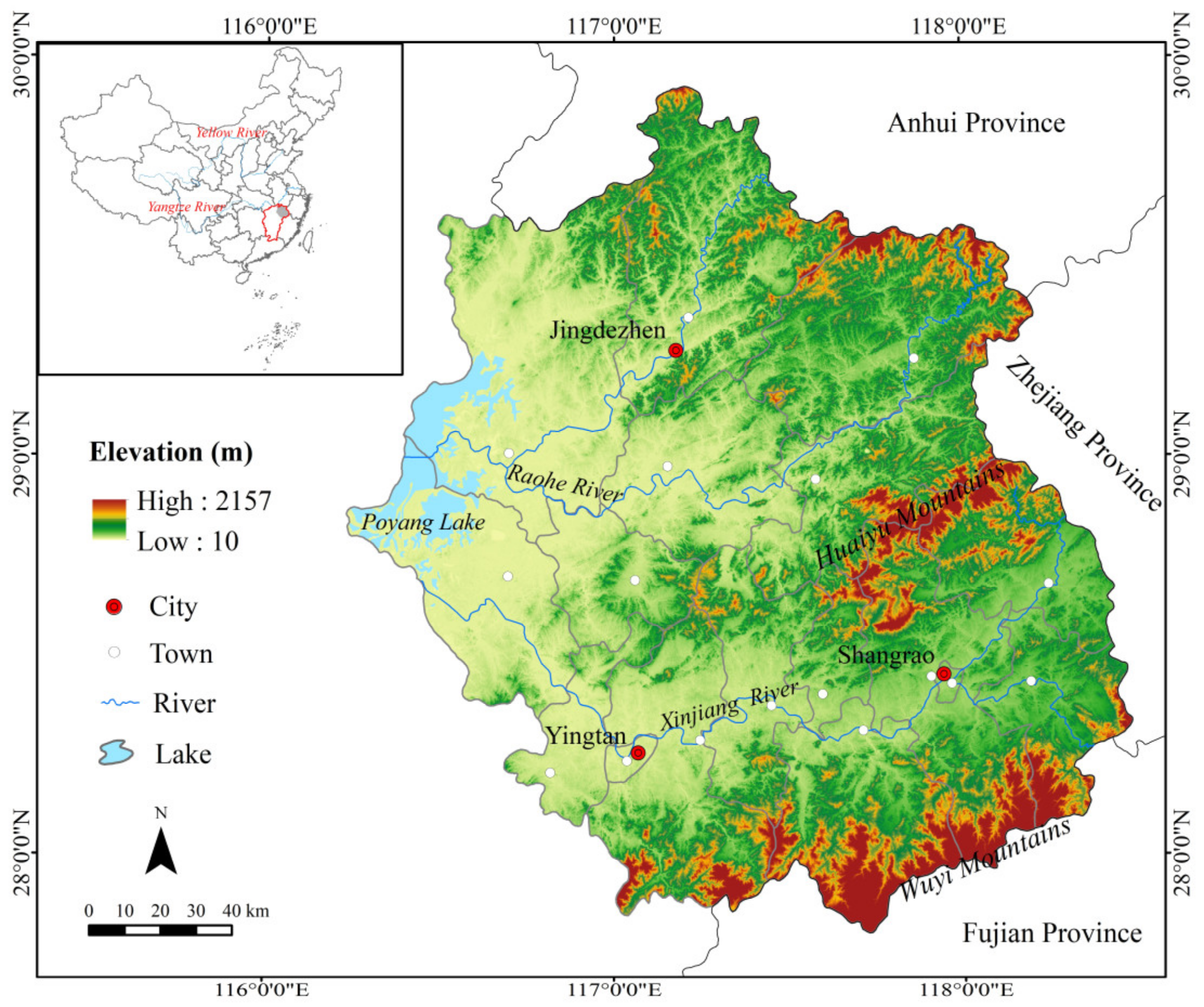
To achieve the objective, a flowchart demonstrating the overall methodology of this research is shown in Figure 1.

2.1. The Study Area

The research area of this study is located in northeast Jiangxi, China, including three cities, namely, Jingdezhen, Shangrao, and Yingtan, and encompassing 19 counties. The terrain inclines largely from the east, composed of a series of northeastern striking mountains and interbedded basins, to the west, where Poyang Lake is situated. The mountain-basin landscape in the east mainly includes three mountain ranges—the Wulong Mountains in the north, the Wuyi Mountains in the south, and the Huaiyu Mountains in the central east. The highest point in the region is Huanggang Mount, the peak of the Wuyi Mountains in Yanshan County, with an altitude of 2157 m. The lowest point is Poyang Lake in the west of the region, with an altitude of nearly 10 m. The water system is well-developed in the study area where the main rivers are Xinjiang, Raohe and their tributaries flowing from east to west into Poyang Lake (Figure 2).

The study area belongs to the subtropical monsoon climate zone. The annual average temperature is around 17 °C. The average temperatures in January and July are about 5 and 29 °C, respectively. Precipitation generally decreases from east to west, with an annual average precipitation of more than 1600 mm.

The main land use and cover types are croplands, forests and woodlands, grasslands, water bodies and artificial areas. Here, woodlands encompass about 19,651.57 km², including mixed forests (11,041.29 km²), coniferous forest (2854.00 km²), bamboo forests (1943.52 km²) and shrublands (2839.05 km²).

2.2. Data

The data used in this study consist of two types: field data obtained from the field surveys and multiresolution satellite images.

2.2.1. Field Data

Two field campaigns were conducted, respectively, during 25–31 October 2019, and 5–18 October 2020, and 28 plots of woodlands and forests (conifers and mixed forests) were measured, including CC, diameter at breast height (DBH), canopy height and tree species and numbers, which will be used for biomass calculation in future.

2.2.2. Multiresolution Satellite Data

While selecting satellite images for vegetation-related research and land cover mapping, phenology is a crucial factor to consider [13,19,21,30,31]. It is natural that herbaceous vegetation grows together with trees in forests and woodlands. Favored by a humid and warm climate, herbaceous vegetation in Jiangxi flourishes in spring, is full of vigor in summer, but withers in late autumn and dries in winter. One may think it reasonable to select winter images for forest research as there is no influence of herbaceous vegetation. Nevertheless, one key factor lies in that most broadleaf trees become leafless, and the sun-elevation angle is so low at that time that the impact of mountain shadow has to be taken into account. Hence, it came to our knowledge that late autumn, e.g., November, is the best month for forest/woodland research as influences of herbaceous vegetation can be reduced and deciduous trees are still green. Another advantage is that the study area becomes dry from November onwards, and there is high possibility to acquire cloud-free satellite images in this month. Therefore, in consideration of all these reasons, November Landsat images were acquired for our study.

As required by multiscale research [13,31] and in order to achieve our objectives, multiresolution and multisensor remote sensing data were prepared as follows:

• Very high-resolution images available on Google Earth (©Google: https://www.google.com/earth/, accessed on 2 April 2021).
• Four scenes of Landsat 8 OLI images (30 m) with Pass/Row Nos. 120/40 and 120/41 acquired on 16 November 2019, and three with Pass/Row No 121/39 and 121/40 on 23 November 2019, were obtained from the USGS data server (https://glovis.usgs.gov/, accessed on 9 March 2020).
• MODIS MOD13Q1 data with frame No h28v06 (250 m, vegetation index 16-day composite product) of a 20-year period from March 2000 to February 2020 were obtained from USGS data server (https://lpdaac.usgs.gov/, accessed on 15 March 2021), and the NDVI data of each month within a 20-year period were extracted to form the NDVI time-series dataset.

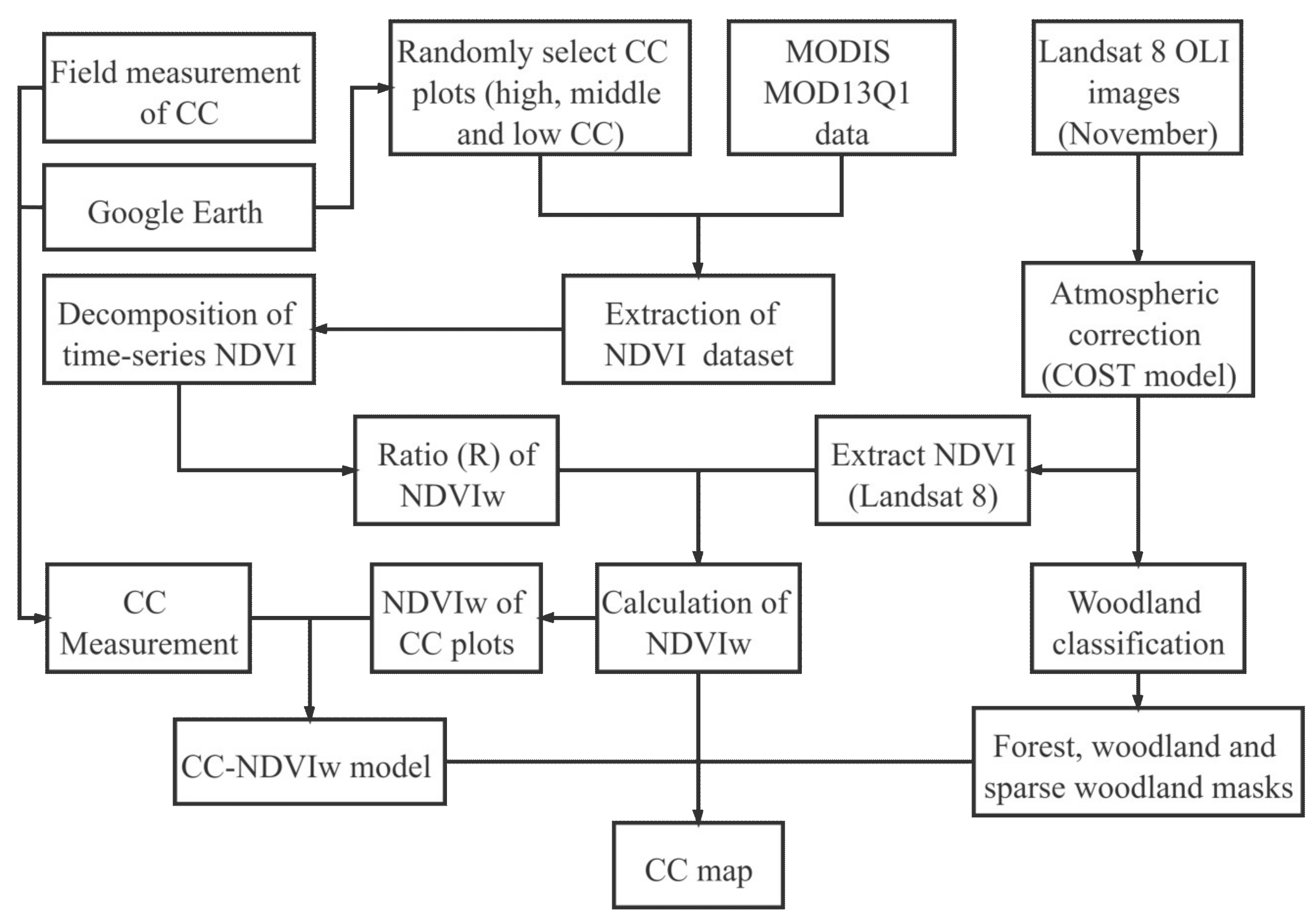
2.3. Development of the CC-NDVI_W Model

A number of vegetation indices such as NDVI, SAVI, SARVI, WDRVI, EVI, and Generalized Difference Vegetation Index (GDVI) have been developed and widely applied in different domains of research, especially in vegetation monitoring [13,27,28,29,31,32,33,34,35,36]. Wu, et al. [13], performed a regression analysis to couple different vegetation indices with CC and concluded that NDVI performed better in building model with CC than other vegetation indices. Therefore, following their conclusion, NDVI, or rather, its woody component, NDVI_W, was selected for CC modeling in this research. The detailed procedure and steps for the development of the CC-NDVI_W model are as follows.

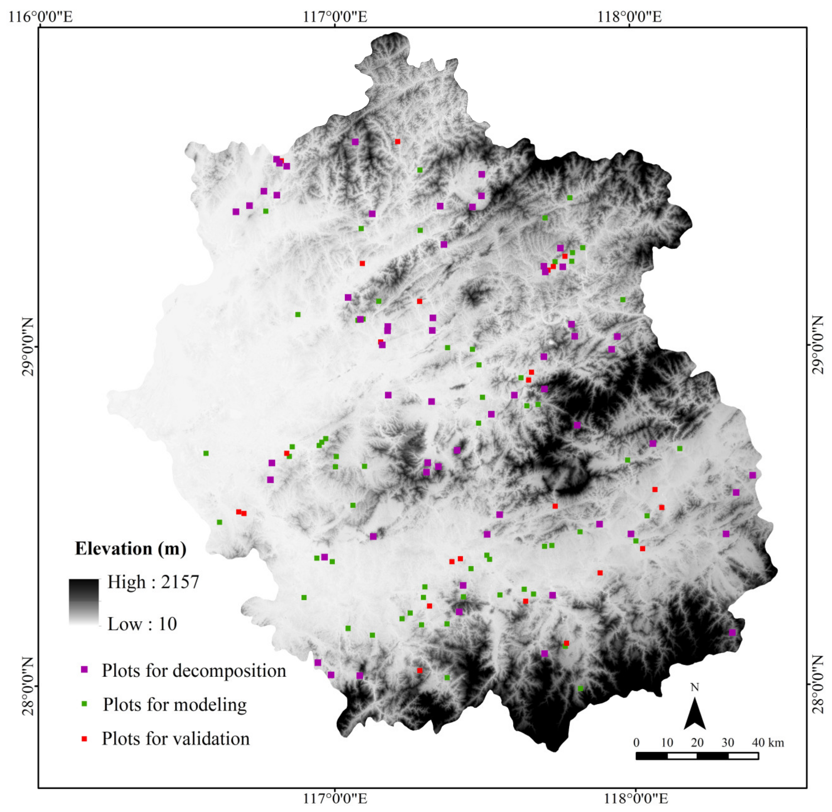
2.3.1. CC Measurement

(1)

CC plots for modeling

The measurement of CC is the key to the establishment of the model and requires representative plots for sampling. In different geographical backgrounds, CC of woodlands has been differently classified by different authors or institutions. In consideration of the climatic conditions in Jiangxi and previous studies, woodland cover in the study area was divided into three categories: forests when CC is greater than 60% (CC_H), medium woodlands when CC is between 25 and 60% (CC_M), and sparse woodlands when CC is 1–25% (CC_L).

The first step was to conduct field campaigns to measure CC of conifers, deciduous species and bamboo across the study area in October 2019 and October 2020. However, due to the complexity of the natural conditions, including landform, canopy interlayer and inaccessibility to the plots of the mixed forests, it was extremely difficult to find reasonable 30 × 30 m² plots, not to mention the full-size ones (100 × 100 m²) on the ground. The 28 measured plots varied from 10 × 10 m² to 30 × 30 m² in size, and the two directions of canopy diameters were used to calculate CC. Unfortunately, five measured dense forest plots of CC reach >100%, mainly incurred from the overlap of canopies with each other. Hence, these five abnormal plots were removed and not used for modeling. The other 23 plots were more or less usable as they are close to those measured on Google Earth, with about 5–12% of difference.

It should be mentioned that under the mature tree canopies, no matter whether they are mixed (Cinnamomum camphora, Schima superba, Liquidambar formosana, Castanea mollissima Blume, Quercus palustris) or coniferous (Pinus massoniana or Pinus elliottiiforests) forests, mid-and young-age trees were rarely observed in the field except for thorns, brambles and rattan vegetation inside the plots. In the young conifer plots, only pure young pines (Pinus massoniana), at ages of about 6–10 years, were found.

The second step was carried out using Google Earth, on which high-resolution (e.g., 0.5–2m) satellite images were available. We considered that this would be better since tree canopy could be recognized and parameterized easily in the forests and woodlands. Thus, 40 plots with an area of 1 ha (100 × 100 m² = 1 ha) were randomly selected in the mixed forests, conifers and woodlands at different CC levels—i.e., high CC (>60%), medium CC (25–60%) and low CC (1–25%), denoted as CC_H, CC_M and CC_L, respectively, on Google Earth. A screenshot function was used to capture the images of these plots. We then imported them into Photoshop, and after discarding the color information, all these plots of images were converted into black and white. An adjustment of the brightness and contrast of the image followed—for example, for each image, the brightness and contrast were uniformly increased to 120 (150 at maximum) and 95 (100 at maximum), respectively. After this processing, the tree canopy (dark) in the sample plot could be clearly separated from other ground features, such as soil and herbaceous vegetation (white). Through the Density Slice tool of ENVI (an image processing package: ©Harris Geospatial Solutions, Inc., https://www.l3harrisgeospatial.com/, accessed on 2 April 2021), the proportion of canopy covered areas in the sample plot could be obtained, and this is the CC we were looking for (Figure 3). This method is appropriate for CC_H, where the plots are filled with tree canopies, and herbaceous vegetation is generally hidden under the canopies, which will not affect the reading of the crown area.

The warm and humid climate favors the vigorous growth of herbaceous vegetation in the study area and even in late autumn it is still green to some extent. In the cases of CC_M and CC_L, such vegetation will definitely influence the recorded signal by sensors as it is a mixture of tree canopies and herbaceous vegetation. If we used a satellite-based vegetation index, e.g., the NDVI, to study CC, herbaceous vegetation would be a problematic issue.

To sort out this issue, we used plot dichotomy to deal with CC_M and CC_L cases. The procedure for this method was first to randomly select a number of candidate areas. Then, inside the selected area, plot(s) were carefully chosen without or with very little herbaceous vegetation, which was distinct from woody trees with dense and concentrated crowns while soil was clear. We defined the tree canopy part of the plot as a closed vector polygon on Google Earth. The area of this polygon was actually the CC of the CC_M and CC_L cases and the left of the plot was soil with low vegetation cover.

Therefore, in total 63 plots of CC were made available for the successive modeling, where 45 plots were dedicated to modeling and 18 plots were used for model validation.

(2)

CC plots for time-series analysis

With the same operation, 60 large plots with sizes of four ha (200 × 200 m²) were also defined on Google Earth at different CC levels, i.e., 20 plots for each category of CC_H, CC_M and CC_L. These plots were used for NDVI sampling in the successive time-series decomposition analysis with MODIS data to estimate the woody component of the observed NDVI. When selecting these sample plots, it was necessary to ensure their spatial representativeness to avoid farmland and mountain terraces, forest fire and deforestation activities so that the plots were not affected by other disturbing features and could be useful.

(3)

CC plots for final CC map validation

To validate the final product of this research, the CC map derived from Landsat images, a third independent group of 24 CC plots with a spatial size of 30 × 30 m² was defined on Google Earth.

The locations of all these three groups of plots are shown in Figure 4.

2.3.2. Atmospheric Correction of Landsat Data

Already orthorectified by the provider, it is only necessary to conduct atmospheric correction for these Landsat 8 OLI images. Radiation transmission is affected by atmospheric scattering and absorption [13,37,38]. Atmospheric correction is used to remove or to minimize such effects in images, and at the same time, to convert the at-satellite solar radiance in digital number (DN) into surface reflectance [13,37,38,39]. Atmospheric correction methods mainly include the radiative transfer code, ground wave measured data regression correction, the histogram minimum value removal, and the image-based DOS (dark-object subtraction) model [33] and its improved version, the COSine Theta (COST) model (in which theta is the zenith angle θ) developed by Chavez [37]. The DOS model only corrects the additive scattering and not the multiplicative transmittance effect [37]; additionally, it may produce an overcorrection and not be applicable in images without dark objects [38]. The COST model provides a reliable image-based approach to correct additive scattering and multiplicative transmittance effects, and it is hence proper for application in vegetation research by remote sensing [13,37,38,40].

In this paper, the COST model was applied for atmospheric correction, i.e., to remove or reduce the haze effects in the at-satellite spectral radiance and at the same time to convert the radiance into surface reflectance [37]. Wu [38] simplified the correction equation of the COST model, and for band i, it can be expressed as:

$${{\displaystyle R}}_i=\frac{\pi }{{{\displaystyle E}}_{oi}{{\displaystyle \cos }}^2\theta }•\frac{{{\displaystyle L}}_{iMax}-{{\displaystyle L}}_{iMin}}{{{\displaystyle DN}}_{iMax}}({{\displaystyle DN}}_i-{{\displaystyle DN}}_{hi})$$

(1)

R_i: spectral reflectance of the surface of band i;

E_oi: maximum solar spectral irradiance of band i;

θ: solar zenith angle;

L_iMax and L_iMin: the maximum and minimum spectral radiances of band i;

DN_iMax: the maximum digital number (DN) of pixel of band i;

DN: DN value of pixel of band i;

DN_hi: the haze value of pixel of band i.

In this atmospheric correction, we used the band minimum as the haze effect. After correction, NDVI of five forest patches increased from 0.61–0.71 to 0.78–0.84. These corrected NDVI values were considered normal and reliable.

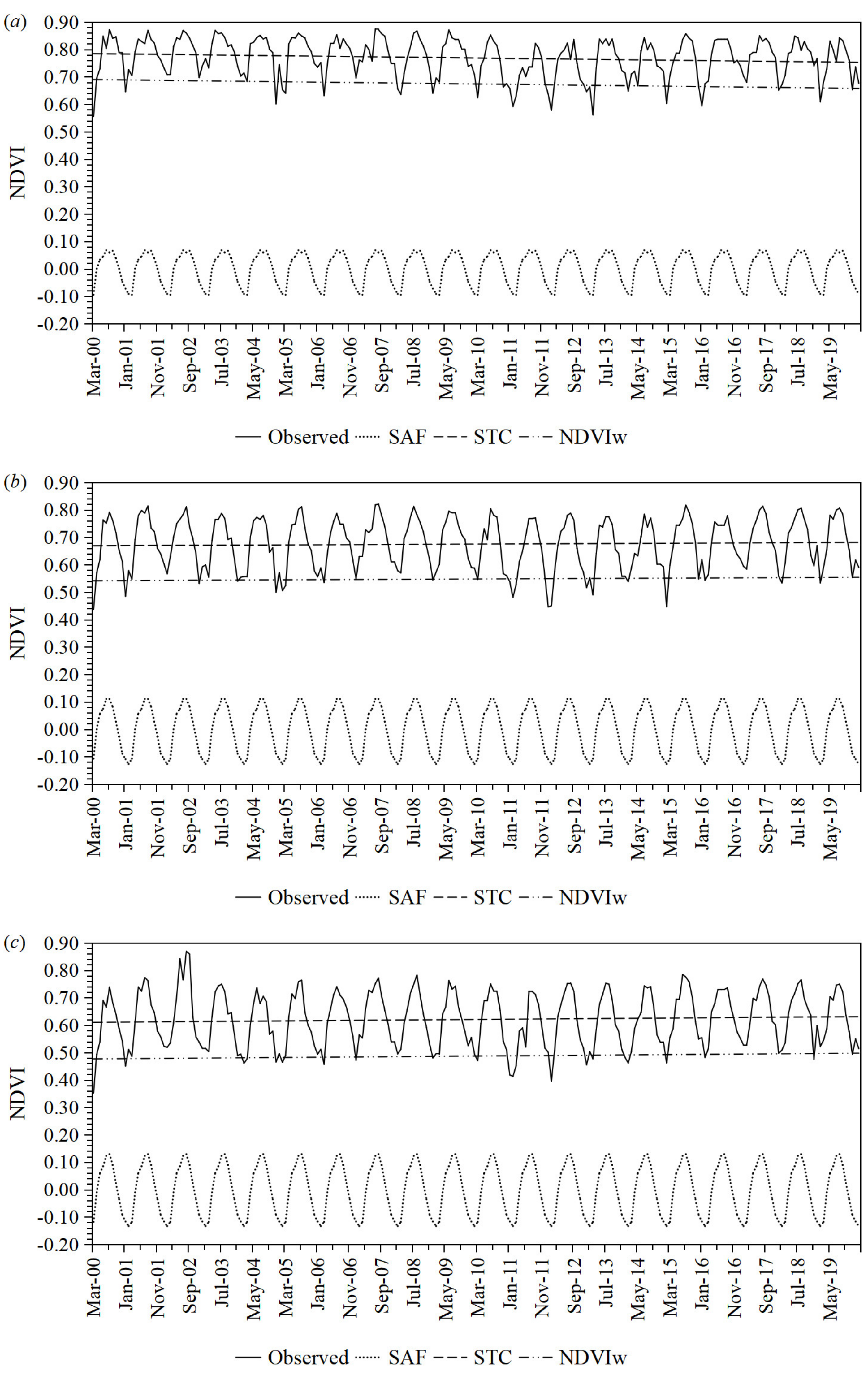
2.3.3. Decomposition of Time-Series MODIS NDVI

As we planned to use Landsat data for CC-NDVI_W modeling, the purpose of this decomposition analysis using the time-series MODIS NDVI dataset was to partition the woody component from the herbaceous vegetation, or rather, to calculate the ratio between the woody component and the satellite observed NDVI. We can thence apply this ratio to Landsat NDVI for extraction of the Landsat woody NDVI (NDVI_LW).

Roderick et al. [41] and Lu et al. [42] extracted NDVI_W by the moving average method to obtain the baseline of NDVI time-series data, thus realizing the partition of woody and herbaceous components. They attributed the baseline of the trend to the woody vegetation and the seasonal signal to the understory herbaceous vegetation. Therefore, they decomposed the NDVI time-series dataset (F) into three components: trend (T), seasonal (S), and irregular variable (E). At a given time t, F can be expressed as:

$$F(t)=T(t)+S(t)+E(t)$$

(2)

Shifting T by a constant K to get the baseline, this is actually the woody component of the observed NDVI. K is the absolute value of the minimum seasonal component for two consecutive years. Then, we have the following equation:

$$NDVI\mathrm{w}=T-K$$

(3)

Our study followed these concepts and used the Statistical Product and Service Solutions (SPSS), a powerful statistical software platform developed by IBM (https://www.ibm.com/analytics/spss-statistics-software, accessed on 9 April 2021), to perform the decomposition analysis using the time-series MODIS NDVI dataset. The 60 4-ha plots, more clearly, 20 plots for each of the three categories CC_H, CC_M, and CC_L which were randomly defined in forests, medium woodlands and sparse woodlands on Google Earth, were saved as vector polygons, and then imported into ENVI and converted into regions of interest (ROIs) of three categories as previously defined.

For the MODIS NDVI product, MOD13Q1, from March 2000 to February 2020, a total of 240 scenes were imported one by one into ENVI to extract the average NDVI for each defined CC category from each NDVI image using the 20 large plots of ROIs of CC_H, CC_M, and CC_L, respectively. The average NDVI dataset of each category with a time span of 240 months was hence prepared. Then, the SPSS package was employed again to conduct the decomposition analysis of the NDVI dataset of 20 high CC (CC_H), 20 CC_M and 20 CC_L plots separately. In the decomposition process, four new sequences were decomposed—namely, the seasonal factor sequence (SAF), seasonal adjustment sequence (SAS), smooth trend cycle sequence (STC), and irregular (error) component sequence (ERR). These sequences correspond to Equation (2): SAF = S, STC = T, ERR = E. Therefore, Equation (3) can be expressed as:

$$NDVI\mathrm{w}=T-K=STC-K$$

(4)

SAS was obtained by deleting the seasonal variations in the original sequence. SAS = OS-SAF. OS is the original value of NDVI. The same operation was carried out for the NDVI dataset of the CC_M and CC_L plots, respectively, and the decomposition results are shown in Figure 5. It can be seen that the K values of the CC_H, CC_M, and CC_L plots are 0.0947, 0.1272, and 0.1335, respectively.

Using Equation (4), the NDVI_W for any month from March 2000 to February 2020 can be calculated. Since Landsat images used for modeling in this paper were acquired in November, it was necessary to calculate the NDVI_W of November for all these three types of plots during the 20-year period. Then, the ratio R of woody NDVI to the satellite observed NDVI was calculated as follows:

$$R=(NDVI\mathrm{w}/NDVI)\times 100\%$$

(5)

According to the above formula, the R values of the CC_H, CC_M, and CC_L plots in November were 0.8774, 0.8462 and 0.8338, respectively.

2.3.4. Derivation of Landsat NDVI_LW

The atmospherically corrected Landsat images of November 2019 were loaded in ENVI, and the NDVIs corresponding to different R values were calculated, denoted as NDVI_LH, NDVI_LM and NDVI_LL, respectively. The 45 sample plots with 1 ha area as mentioned above were imported into the ENVI. These 45 plot frames, in three classes of CC_H, CC_M and CC_L, were, respectively, converted into ROIs, and denoted as ROI_H, ROI_M and ROI_L. In the NDVI_LH image, the NDVI_LW of each CC_H plot in ROI_H was obtained. The same was effectuated to obtain the NDVI_LW of the other two types of plots, ROI_M and ROI_L.

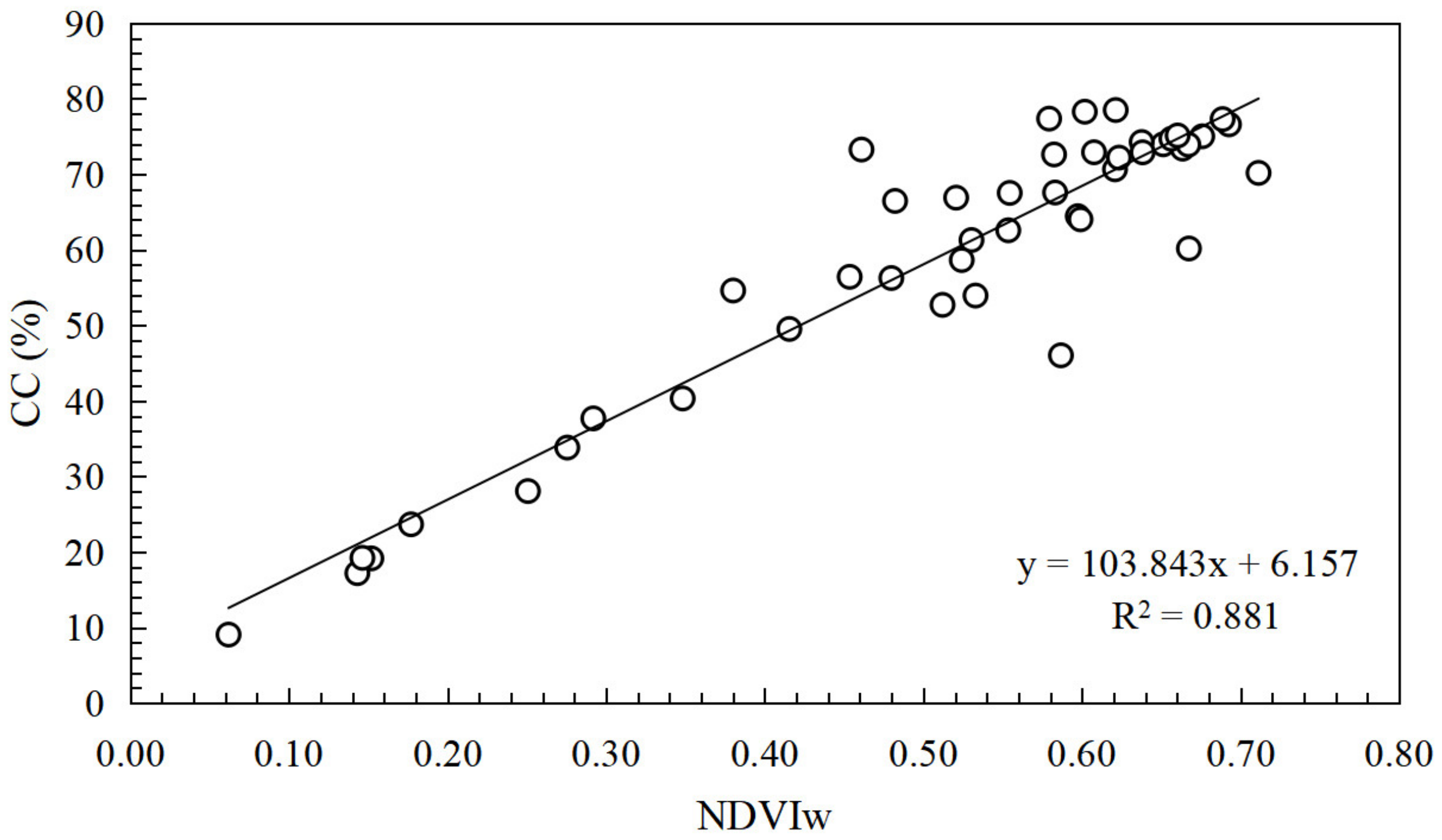
2.3.5. CC-NDVI_W Modeling

The measured CC of the 45 plots and their corresponding NDVI_LW obtained from the above procedure were coupled with a linear regression analysis to construct the CC-NDVI_LW model at the confidence level of 95% (see Figure 6). The regression equation was obtained as follows:

$$CC=103.843 NDV{I}_{LW}+6.157(R^2=0.881)$$

(6)

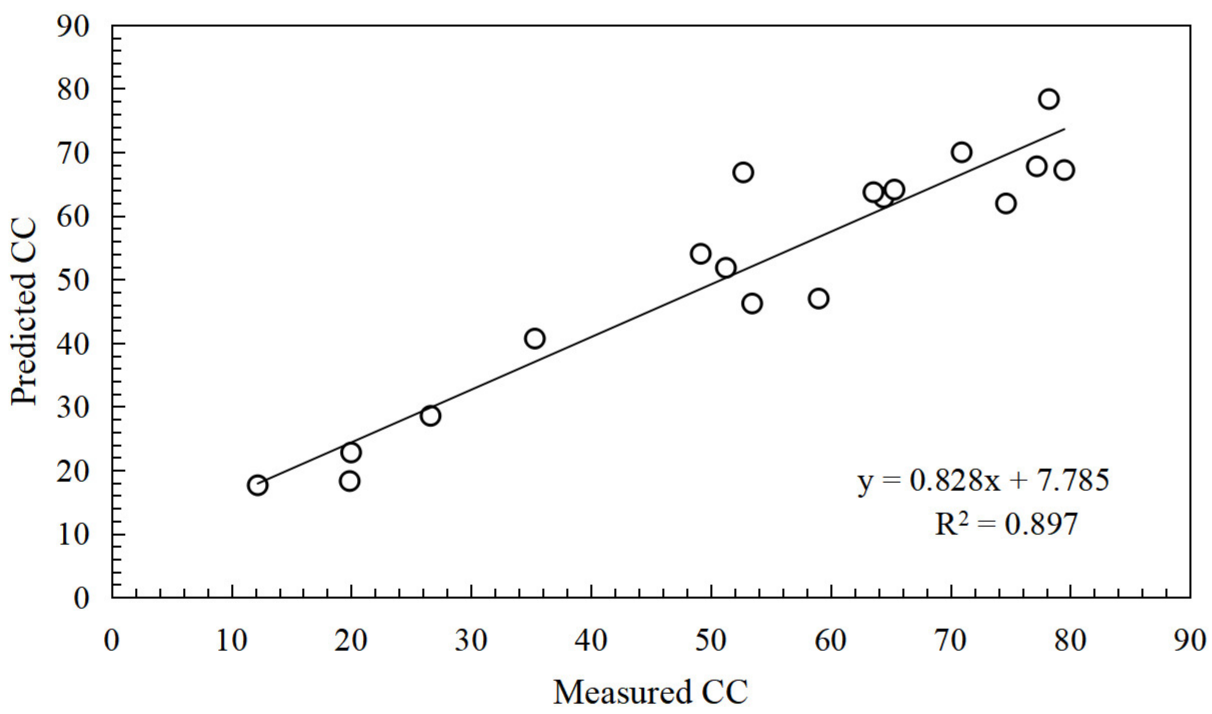
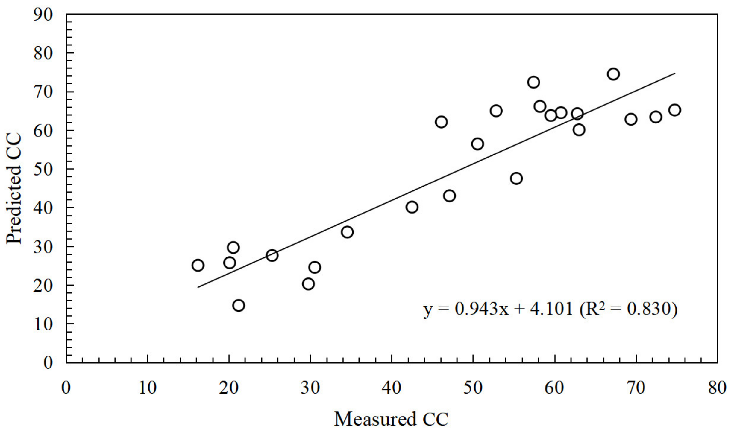
2.3.6. Verification of CC-NDVI_LW Model

As described in the foregoing sections, the 18 remaining CC plots were used as verification samples to validate the above model. We took advantage of Equation (6) to calculate the predicted CC at the verification sample plots and coupled it with the measured CC samples using the linear regression model again at a confidence level of 95% (Figure 7). It is clear that the agreement is extremely high, indicating that the developed CC-NDVI_W model is capable of achieving reliable CC prediction.

2.4. Application of CC-NDVI_LW Model for CC Mapping

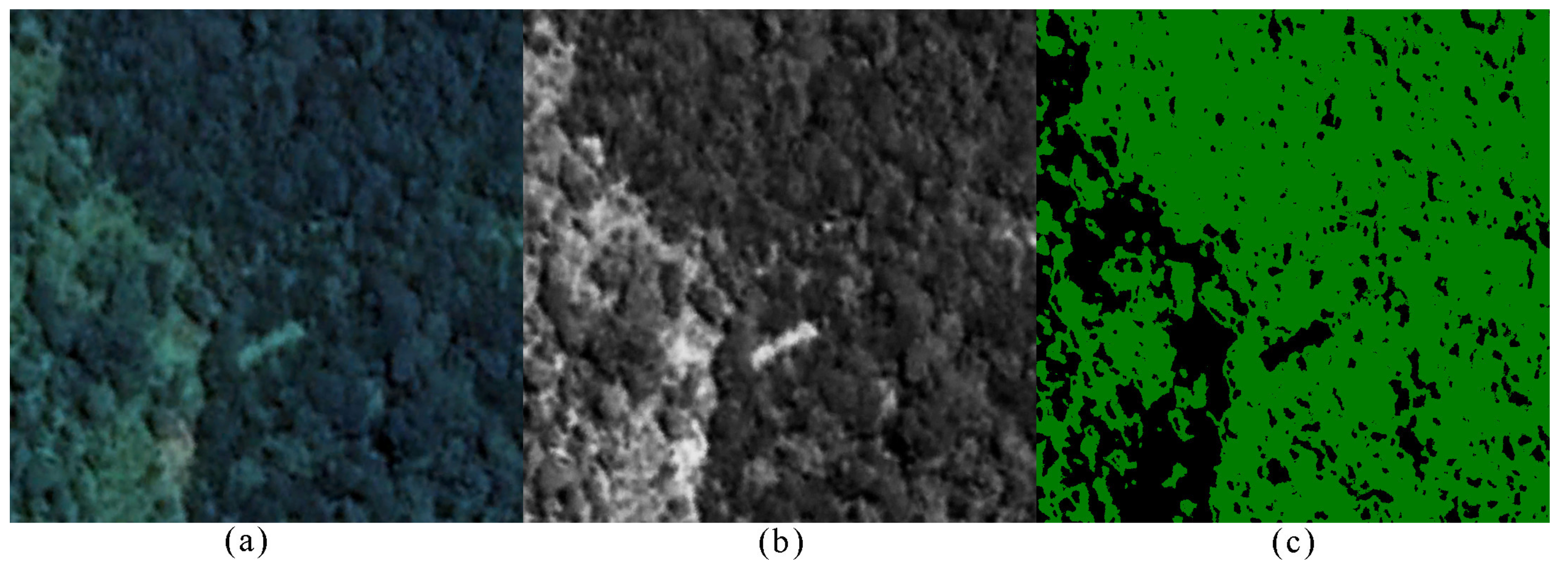
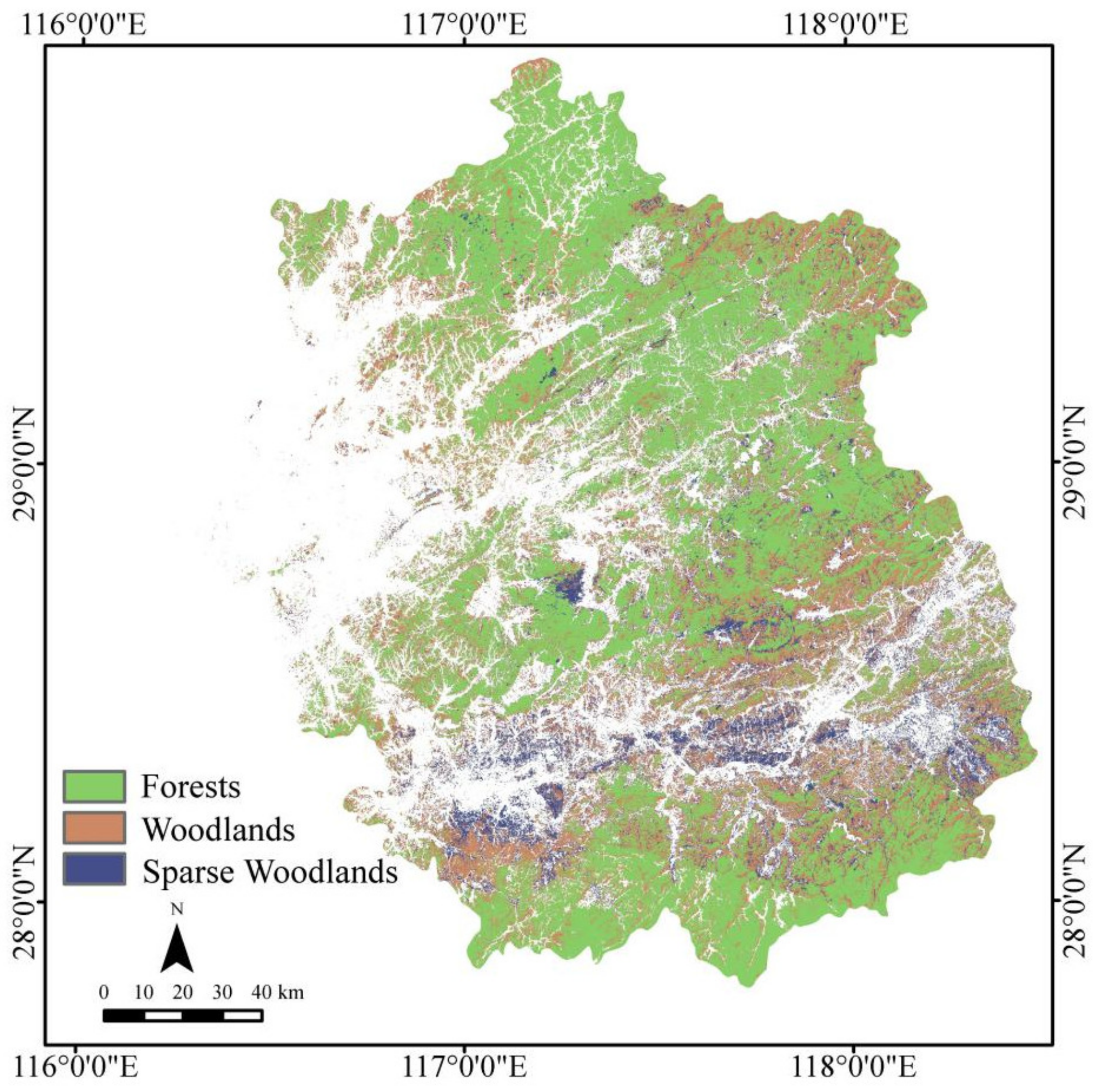
2.4.1. Woodland Classification

To apply the developed model for estimating woodland CC of the study area, an essential procedure is to derive different CC level masks where woody NDVI can be, respectively, calculated from the Landsat NDVI. Based on an intensive land cover mapping, all woodlands and forests of the study area were extracted to build a woodland mask. As divided during the CC classification, samples of CC_H, CC_M, and CC_L were further defined in forest and woodland areas in Landsat images with reference to Google Earth, and a supervised classification with a random forests algorithm was further carried out under the woodland mask. All woodlands were hence divided into three levels, i.e., forests, medium woodlands and sparse woodlands in northeast Jiangxi in terms of the CC levels, i.e., CC_H, CC_M, and CC_L.

2.4.2. Model Application to Estimate Regional-Scale CC

The produced CC_H, CC_M, and CC_L zones were extracted to create three canopy cover masks, denoted as Mask_H, Mask_M and Mask_L. Under these three different masks, the woody NDVI (i.e., NDVI_LW) was, respectively, calculated for each pixel using the above decomposition ratios.

The CC-NDVI_LW model was applied to each of these three zones of NDVI_LW to produce CC, and then, a mosaic was conducted to merge all these three zones of CC to constitute the CC map.

This CC map was verified against the independent group of 24 plots of CC (Section 2.3.). If the agreement was good (e.g., >80%), the CC map was thereby validated. Otherwise, it would be necessary to repeat the whole procedure until the agreement was satisfactory.

3. Results and Discussion

3.1. CC Measurement

Among the 63 measured plots of CC, their distributions in different CC levels were, respectively, 8 plots at CC_L, 19 plots at CC_M, and 37 plots at CC_H. Measuring field CC was a tough job and less accurate than when using Google Earth due to the complex landform and difficulty of accessing the plots. Hence, we used a combination of the field measured CC with those from Google Earth for CC-NDVI_W modeling.

The CC measurement method can also be calculated by directly measuring the canopy diameter of the canopy in field and on Google Earth using a formula proposed by Wu et al. [13]. This method is simple and feasible, but it is cumbersome to measure each tree. However, using the method of this paper described in Section 2.3.1 to process the plots can greatly improve the measurement efficiency and is more suitable for areas where there are luxuriant trees. The study area is complex in landform and composed of both mountains and basins; nevertheless, it is essential to select relatively flat areas for CC measurements. If plots were selected in the shadow of the north hillside with steep slopes, CC measurement and NDVI_W would be affected, as would the CC estimation from Landsat data. In addition, disturbance from human activities such as deforestation, burning, terrace reclamation, ore mineral exploitation, etc., which directly affects the value of NDVI_W, should be avoided.

The acquisition time difference between Landsat images and the very high-resolution data on Google Earth has to be considered. If CC and NDVI_W were found to be inharmonious, it was necessary to check whether there was sudden change in the plot. If NDVI_W was derived from images before or after the change observed on Google Earth, there would be, respectively, a high NDVI_W versus a low CC or a low NDVI_W versus a high CC. These abnormal cases should be excluded.

3.2. The Importance of Decomposition of Time-Series Dataset

While extracting NDVI_W, the influence from herbaceous vegetation has to be taken into account as it is still partially green in the study area even in late autumn. Although we had screened the sample plots to minimize herbaceous vegetation, it was impossible to completely eliminate its influence on NDVI. The direct extraction of NDVI in the sample plots from the November Landsat data would be risky and not be recommended. For this reason, it is critical to conduct the decomposition processing of time-series NDVI to minimize the impact of herbaceous vegetation on NDVI_W. Our results may be applied to extract woody NDVI in any month of the year as we have obtained the year-round woody component, i.e., the baselines of forests, medium woodlands and sparse woodlands as shown in Figure 5.

3.3. Woodland Classification and NDVI_W Maps

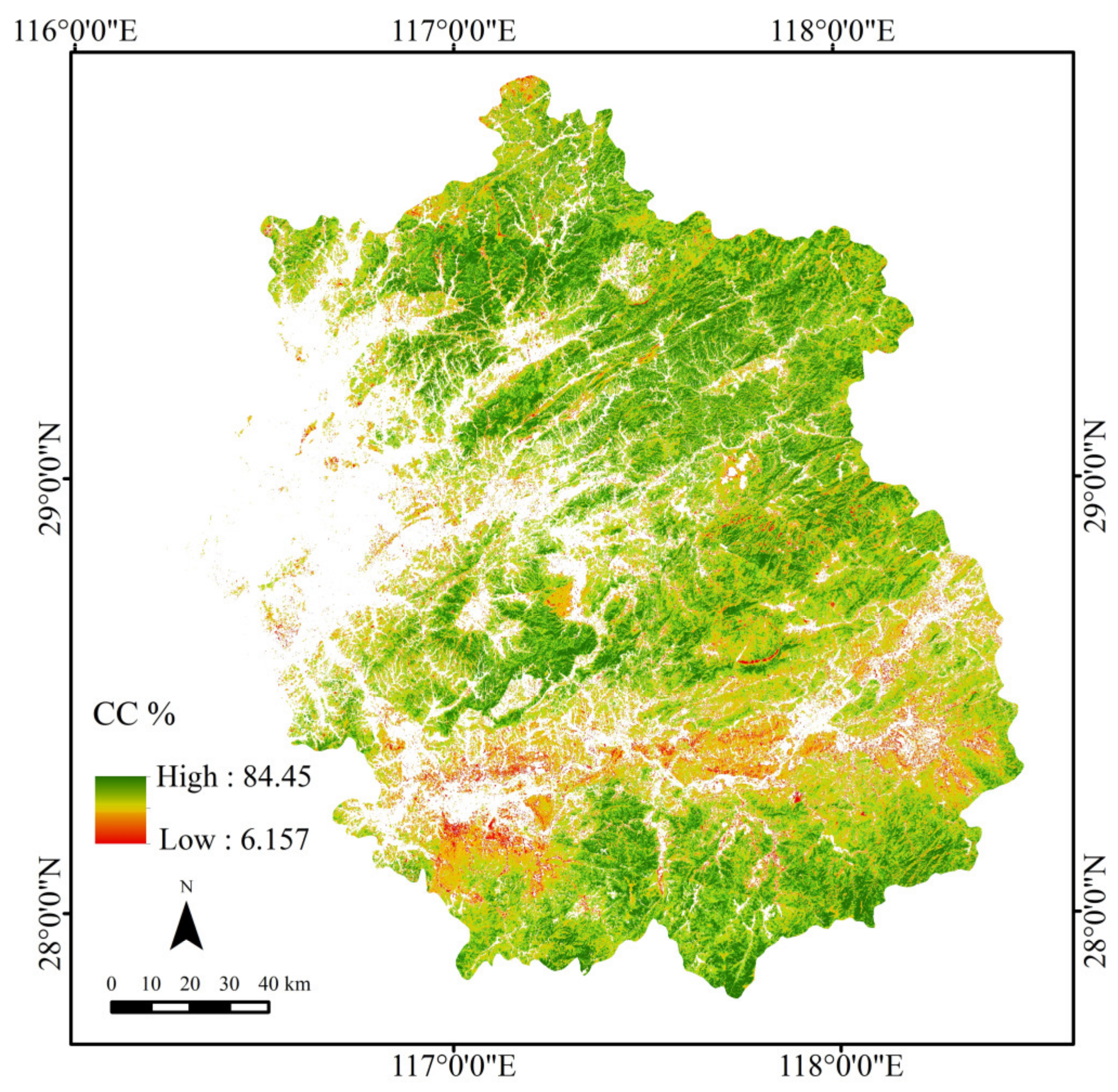
The classification map of woodlands was the basis for generating CC map. Using the abovementioned approach, the four scenes of Landsat 8 images acquired in November 2019 were classified into forests (CC_H), medium woodlands (CC_M) and sparse woodlands (CC_L) with accuracies of 90.17, 90.12, 94.23 and 91.78%, respectively. The three classes of woodlands of the four scenes were mosaicked to constitute the regional woodland map (Figure 8) and at the same time to produce three classes of woodland masks: forests, medium woodlands and sparse woodlands. These masks were used for derivation of NDVI_W of each woodland class with its corresponding woody NDVI ratio R. After mosaicking, a Landsat NDVI_W map was also produced.

3.4. CC Mapping

To demonstrate the applicability of the developed CC-NDVI_W model, the latter was applied to the Landsat-derived NDVI_LW under the three woodland masks to predict CC and the result, the CC map, is presented in Figure 9.

For validation purpose, corresponding to the third group of 24 measured CC plots from Google Earth, the predicted 24 CC values from the CC map were extracted and both were coupled using linear regression analysis again at the confidence level of 95%. Fortunately, the agreement reaches 83.0% (Figure 10), implying that using the proposed approach, the predicted forest and woodland CC is reliable, or rather, the developed CC-NDVI_W model is operational and able to relevantly estimate CC with high accuracy in northeast Jiangxi.

3.5. Possibility of Extension

The multiscale approach for regional scale CC mapping has clear advantages—i.e., it can be applied for CC estimation in any month of the year if cloud-free high-resolution images are available. It is known that wood species are normally Cunninghamia lanceolata, Pinus massoniana for coniferous forests, Cinnamomum camphora, Pinus massoniana, Schima superba, Pinus elliottii, Cunninghamia lanceolata, Liquidambar formosana, Castanea mollissima Blume, and Quercus palustris for mixed forests, and Phyllostachys pubescens, Phyllostachys heteroclada Oliver, and Phyllostachys stimulosa for bamboo forests in the study area. Actually, from north to south and from east to west, forests are more or less similar in the whole of Jiangxi Province, and even in the whole of south China. The only difference lies in the abundance of broadleaf trees between the southern coastal provinces, such as Guangdong and Guangxi, which are favored by abundant rainfall, and those inside the Yangtze River Watershed, e.g., Hunan, Hubei, Jiangxi and Anhui.

Thus, the approaches developed in this study are most likely extendable to south China and the CC-NDVI_W model is directly applicable to the whole of Jiangxi and even Hunan, Anhui and Zhejiang for regional and subnational CC mapping.

Though global-scale tree cover data of 500 m resolution have been made available by NASA, which were derived from MODIS data [21], our approach can be considered as a complement to theirs to derive regional- and subnational-scale forest and woodland CC by high-resolution satellite data. Such a product may provide more useful information for forest resource monitoring and management for local and regional authorities.

4. Conclusions

This paper demonstrated development of a multiscale forest and woodland CC mapping approach based on the derivation of woody NDVI through time-series decomposition analysis and construction of the CC-NDVI_W model in northeast Jiangxi. This approach provided a simple, fast, and regional-scale CC estimation and mapping possibility. Compared with the traditional manual measurements, the developed method has evident advantages, i.e., cost-effectiveness, not time-consuming, and especially, possibility of year-round CC mapping. Theoretically, the developed model appears to be applicable for characterization of forests and woodlands in the whole of Jiangxi. Moreover, as long as there is a CC classification map and corresponding NDVI_W data, the model can be extended to other subtropical monsoon climate regions where coniferous and mixed forests coexist, for example, in south China, thanks to the similarity in woody species and climate conditions there.

Moreover, after we encountered a difficulty in implementing the field measurement of CC, we employed Google Earth as an alternative to supplement the measurement so that this study provides an operational example of integration of field measurement with Google Earth. To overcome the field difficulty of measurement, use of an unmanned aerial vehicle (UAV) is a good option, and this is going to be conducted in our next step of research.

References

1. Jennings, S.; Brown, N.; Sheil, D. Assessing forest canopies and understorey illumination: Canopy closure, canopy cover and other measures. For. Int. J. For. Res. 1999, 72, 59–74. [Google Scholar] [CrossRef]
2. Korhonen, L.; Korhonen, K.T.; Rautiainen, M.; Stenberg, P. Estimation of forest canopy cover a comparison of field meas-urement techniques. Silva Fenn. 2006, 40, 577–588. [Google Scholar] [CrossRef] [Green Version]
3. Korhonen, L.; Hadi; Packalen, P.; Rautiainen, M. Comparison of Sentinel-2 and Landsat 8 in the estimation of boreal forest canopy cover and leaf area index. Remote. Sens. Environ. 2017, 195, 259–274. [Google Scholar] [CrossRef]
4. Gill, S.J.; Biging, G.S.; Murphy, E.C. Modeling conifer tree crown radius and estimating canopy cover. For. Ecol. Manag. 2000, 126, 405–416. [Google Scholar] [CrossRef] [Green Version]
5. Cade, B.S. Comparison of Tree Basal Area and Canopy Cover in Habitat Models: Subalpine Forest. J. Wildl. Manag. 1997, 61, 326. [Google Scholar] [CrossRef]
6. O’Brien, R. Comparison of Overstory Canopy cover Estimates on Forest Survey Plots; US Department of Agriculture, Forest Service, Intermountain Research Station: Ogden, UT, USA, 1989; Volume 417, pp. 1–5. [Google Scholar]
7. Yu, Z.; Ustin, S.L.; Zhang, Z.; Liu, H.; Zhang, X.; Meng, X.; Cui, Y.; Guan, H. Estimation of a New Canopy Structure Parameter for Rice Using Smartphone Photography. Sensors 2020, 20, 4011. [Google Scholar] [CrossRef] [PubMed]
8. Knyazikhin, Y.; Martonchik, J.V.; Myneni, R.B.; Diner, D.J.; Running, S.W. Synergistic algorithm for estimating vegetation canopy leaf area index and fraction of absorbed photosynthetically active radiation from MODIS and MISR data. J. Geophys. Res. Space Phys. 1998, 103, 32257–32275. [Google Scholar] [CrossRef] [Green Version]
9. Kuusk, A.; Nilson, T. A directional multispectral forest reflectance model. Remote. Sens. Environ. 2000, 72, 244–252. [Google Scholar] [CrossRef]
10. Griffin, A.M.R.; Popescu, S.C.; Zhao, K. Using LIDAR and normalized difference vegetation index to remotely determine LAI and percent canopy cover. In Proceedings of the SilviLaser 2008: 8th international conference on LiDAR applications in forest assessment and inventory, Edinburgh, UK, 17–19 September 2008; pp. 446–455. [Google Scholar]
11. Nielsen, D.C.; Miceli-Garcia, J.J.; Lyon, D.J. Canopy Cover and Leaf Area Index Relationships for Wheat, Triticale, and Corn. Agron. J. 2012, 104, 1569–1573. [Google Scholar] [CrossRef] [Green Version]
12. Moličová, H.; Hubert, P. Canopy Influence on Rainfall Fields’ Microscale Structure in Tropical Forests. J. Appl. Meteorol. 1994, 33, 1464–1467. [Google Scholar] [CrossRef] [Green Version]
13. Wu, W.; De Pauw, E.; Helldén, U. Assessing woody biomass in African tropical savannahs by multiscale remote sensing. Int. J. Remote. Sens. 2013, 34, 4525–4549. [Google Scholar] [CrossRef]
14. Bechtold, W.A. Crown-diameter prediction models for 87 species of stand-grown trees in the eastern United States. South. J. Appl. For. 2003, 27, 269–278. [Google Scholar] [CrossRef] [Green Version]
15. Melin, M.; Korhonen, L.; Kukkonen, M.; Packalen, P. Assessing the performance of aerial image point cloud and spectral metrics in predicting boreal forest canopy cover. ISPRS J. Photogramm. Remote. Sens. 2017, 129, 77–85. [Google Scholar] [CrossRef]
16. Nelson, R.F. Detecting Forest Canopy Change a Due to Insect Activity Using 3 Landsat MSS. Photogramm. Eng. Remote. Sens. 1983, 49, 1303–1314. [Google Scholar]
17. FAO. Estimating Biomass and Biomass Change of Tropical Forests: A Primer. Available online: http://www.fao.org/3/W4095E/w4095e00.htm (accessed on 3 May 2020).
18. FAO. Forest Cover Mapping and Monitoring with NOAA-AVHRR and Other Coarse Spatial Resolution Sensors. Available online: http://www.fao.org/3/ae161e/AE161E00.htm (accessed on 3 May 2020).
19. DeFries, R.S.; Hansen, M.C.; Townshend, J.R.G.; Janetos, A.C.; Loveland, T.R. A new global 1-km dataset of percentage tree cover derived from remote sensing. Glob. Chang. Biol. 2000, 6, 247–254. [Google Scholar] [CrossRef]
20. Foody, G.M.; Boyd, D.S.; Cutler, M.E. Predictive relations of tropical forest biomass from Landsat TM data and their transferability between regions. Remote. Sens. Environ. 2003, 85, 463–474. [Google Scholar] [CrossRef]
21. Hansen, M.C.; Defries, R.S.; Townshend, J.R.G.; Carroll, M.; Sohlberg, R.A. Global percent tree cover at a spatial resolution of 500 meters First results of the MODIS vegetation continuous fields algorithm. Earth Interact. 2003, 7, 1–15. [Google Scholar] [CrossRef] [Green Version]
22. Thenkabail, P.S.; Stucky, N.; Griscom, B.W.; Ashton, M.S.; Diels, J.; Van Der Meer, B.; Enclona, E. Biomass estimations and carbon stock calculations in the oil palm plantations of African derived savannas using IKONOS data. Int. J. Remote. Sens. 2004, 25, 5447–5472. [Google Scholar] [CrossRef]
23. Heiskanen, J. Estimating aboveground tree biomass and leaf area index in a mountain birch forest using ASTER satellite data. Int. J. Remote. Sens. 2006, 27, 1135–1158. [Google Scholar] [CrossRef]
24. IPCC (Intergovernmental Panel on Climate Change). The Carbon Cycle and Atmospheric Carbon Dioxide; Cambridge University: Cambridge, UK, 2001; pp. 183–238. [Google Scholar]
25. Hadi; Korhonen, L.; Hovi, A.; Rönnholm, P.; Rautiainen, M. The accuracy of large-area forest canopy cover estimation using Landsat in boreal region. Int. J. Appl. Earth Obs. Geoinf. 2016, 53, 118–127. [Google Scholar] [CrossRef]
26. Trout, T.J.; Johnson, L.F.; Gartung, J. Remote Sensing of Canopy Cover in Horticultural Crops. HortScience 2008, 43, 333–337. [Google Scholar] [CrossRef] [Green Version]
27. Kaufman, Y.; Tanre, D. Atmospherically resistant vegetation index (ARVI) for EOS-MODIS. IEEE Trans. Geosci. Remote. Sens. 1992, 30, 261–270. [Google Scholar] [CrossRef]
28. Huete, A.R.; Liu, H.Q.; Batchily, K.; Leeuwen, W.V. A Comparison of Vegetation Indices Global Set of TM Images for EOS-MODIS. Remote. Sens. Environ. 1997, 59, 440–451. [Google Scholar] [CrossRef]
29. Gitelson, A.A. Wide Dynamic Range Vegetation Index for Remote Quantification of Biophysical Characteristics of Vegetation. J. Plant Physiol. 2004, 161, 165–173. [Google Scholar] [CrossRef] [PubMed] [Green Version]
30. Wu, W.; Zucca, C.; Karam, F.; Liu, G. Enhancing the performance of regional land cover mapping. Int. J. Appl. Earth Obs. Geoinf. 2016, 52, 422–432. [Google Scholar] [CrossRef]
31. Wu, W.; Al-Shafie, W.M.; Mhaimeed, A.S.; Ziadat, F.; Nangia, V.; Payne, W.B. Soil Salinity Mapping by Multiscale Remote Sensing in Mesopotamia, Iraq. IEEE J. Sel. Top. Appl. Earth Obs. Remote. Sens. 2014, 7, 4442–4452. [Google Scholar] [CrossRef]
32. Tucker, C.J. Red and photographic infrared linear combinations for monitoring vegetation. Remote. Sens. Environ. 1979, 8, 127–150. [Google Scholar] [CrossRef] [Green Version]
33. Chavez, P.S. An improved dark-object subtraction technique for atmospheric scattering correction of multispectral data. Remote. Sens. Environ. 1988, 24, 459–479. [Google Scholar] [CrossRef]
34. Huete, A.R. Vegetation Indices, Remote Sensing and Forest Monitoring. Geogr. Compass 2012, 6, 513–532. [Google Scholar] [CrossRef]
35. Wu, W. The Generalized Difference Vegetation Index (GDVI) for Dryland Characterization. Remote. Sens. 2014, 6, 1211–1233. [Google Scholar] [CrossRef] [Green Version]
36. Wu, W.; Mhaimeed, A.S.; Al-Shafie, W.M.; Ziadat, F.; Dhehibi, B.; Nangia, V.; De Pauw, E. Mapping soil salinity changes using remote sensing in Central Iraq. Geoderma Reg. 2014, 2–3, 21–31. [Google Scholar] [CrossRef]
37. Chavez, P.S.J. Image-Based Atmospheric Correction—Revisited and Improved. Photogramm. Eng. Remote. Sens. 1996, 62, 1025–1035. [Google Scholar]
38. Wu, W. Application de la Geomatique au Suivi de la Dynamique Environnementale en Zones Arides. Ph.D. Thesis, Université de Paris 1, Paris, France, 2003. [Google Scholar]
39. Song, W.-W.; Guan, D.-S. Application of five atmospheric correction models for Landsat TM data in vegetation remote sensing. Chin. J. Appl. Ecol. 2008, 19, 769–774. [Google Scholar]
40. Li, H.; Guo, K.; Dan, S.; Lu, Z.; Xu, H. Analysis on spatial and temporal variation of urban heat island effect based on COST model. Sci. Surv. Mapp. 2012, 37, 164–166. [Google Scholar] [CrossRef]
41. Roderick, M.L.; Noble, I.R.; Cridland, S.W. Estimating woody and herbaceous vegetation cover from time series satellite observations. Glob. Ecol. Biogeogr. 1999, 8, 501–508. [Google Scholar] [CrossRef]
42. Lu, H. Decomposition of vegetation cover into woody and herbaceous components using AVHRR NDVI time series. Remote. Sens. Environ. 2003, 86, 1–18. [Google Scholar] [CrossRef]
Figure 1. The overall methodological flowchart applied in this study.
Land 10 00433 g001
Figure 2. Location of the study area—northeast Jiangxi, China.
Land 10 00433 g002
Figure 3. An example of extracting CC using Photoshop and Density Slicing within ENVI. (a) Captured image plot on Google Earth using the screenshot function; (b) discarding of color and enhancement of brightness and contrast of the plot to 120 (150 at maximum) and 95 (100 at maximum), respectively, in Photoshop; and (c) canopy cover rendered by thresholding using the Density Slice tool of ENVI.
Land 10 00433 g003
Figure 4. Locations of the three sets of plots for modeling, decomposition and validation.
Land 10 00433 g004
Figure 5. Decomposition results: (a) forests; (b) medium woodlands; and (c) sparse woodlands. Note: Here “Observed” denotes the original value of MODIS NDVI. X−axis represents months—240 in total; Mar−00 = March 2000 and May−19 = May 2019. SAF—seasonal factor sequence, STC—smooth trend cycle sequence, and NDVIW—woody component of the observed NDVI.
Land 10 00433 g005
Figure 6. CC-NDVILW model calibrated by linear regression analysis.
Land 10 00433 g006
Figure 7. Model validation: agreement between the measured and predicted 18 plots of CC.
Land 10 00433 g007
Figure 8. Woodland classification map of northeast Jiangxi. Note: Forests where CC > 60%—CCH, medium woodlands with CC of 25–60%—CCM and sparse woodlands with CC of 1–25%—CCL.
Land 10 00433 g008
Figure 9. Forest and woodland canopy cover (CC) map of northeast Jiangxi.
Land 10 00433 g009
Figure 10. Agreement between the predicted CC from the Landsat-derived CC map and the independent group of 24 validation plots of CC from Google Earth.
Land 10 00433 g010
Publisher’s Note: MDPI stays neutral with regard to jurisdictional claims in published maps and institutional affiliations.