High-Resolution Monitoring and Assessment of Evapotranspiration and Gross Primary Production Using Remote Sensing in a Typical Arid Region

Abstract

Land surface evapotranspiration (ET) and gross primary productivity (GPP) are critical components in terrestrial ecosystems with water and carbon cycles. Large-scale, high-resolution, and accurately quantified ET and GPP values are important fundamental data for freshwater resource management and help in understanding terrestrial carbon and water cycles in an arid region. In this study, the revised surface energy balance system (SEBS) model and MOD17 GPP algorithm were used to estimate daily ET and GPP at 100 m resolution based on multi-source satellite remote sensing data to obtain surface biophysical parameters and meteorological forcing data as input variables for the model in the midstream oasis area of the Heihe River Basin (HRB) from 2010 to 2016. Then, we further calculated the ecosystem water-use efficiency (WUE). We validated the daily ET, GPP, and WUE from ground observations at a crop oasis station and conducted spatial intercomparisons of monthly and annual ET, GPP, and WUE at the irrigation district and cropland oasis scales. The site-level evaluation results show that ET and GPP had better performance than WUE at the daily time scale. Specifically, the deviations in the daily ET, GPP, and WUE data compared with ground observations were small, with a root mean square error (RMSE) and mean absolute percent error (MAPE) of 0.75 mm/day and 26.59%, 1.13 gC/m² and 36.62%, and 0.50 gC/kgH₂O and 39.83%, respectively. The regional annual ET, GPP, and WUE varied from 300 to 700 mm, 200 to 650 gC/m², and 0.5 to 1.0 gC/kgH₂O, respectively, over the entire irrigation oasis area. It was found that annual ET and GPP were greater than 550 mm and 500 gC/m², and annual oasis cropland WUE had strong invariability and was maintained at approximately 0.85 gC/kgH₂O. The spatial intercomparisons from 2010 to 2016 revealed that ET had similar spatial patterns to GPP due to tightly coupled carbon and water fluxes. However, the WUE spatiotemporal patterns were slightly different from both ET and GPP, particularly in the early and late growing seasons for the oasis area. Our results demonstrate that spatial full coverage and reasonably fine spatiotemporal variation and variability could significantly improve our understanding of water-saving irrigation strategies and oasis agricultural water management practices in the face of water shortage issues.

1. Introduction

Land surface gross primary productivity (GPP) and evapotranspiration (ET) are key parameters for characterizing surface physical and biological processes in ecosystems. A strong coupling relationship exists between GPP and ET. For instance, in corn farmland, the vegetation transpiration components of ET can increase directly with increased GPP and the soil evaporation components of ET can decrease associated with increased GPP [1]. Against the background of human activities and global warming, one of the prerequisites for rational carbon–water management is to have an accurate measure of the ET and GPP characteristics of a terrestrial ecosystem. This understanding plays an essential role in the sustainable development of the regional ecological environment and regional water resource management.

Over nearly a decade, numerous ET measurements for water consumption and GPP measurements for biomass production at single station and global (regional) scales have been derived from remote sensing data with ET models, such as the Surface Energy Balance System (SEBS) [2,3], the two-source energy balance (TSEB) model [4,5], the Penman–Monteith (P-M) [6] and Priestley–Taylor (P-T) equations [7,8], and the Global Land Evaporation Amsterdam Model (GLEAM) [9] and GPP models [10,11]. These have been used to compute water-use efficiency (WUE) for water-resource assessment using GPP divided by ET, which is a key indicator linking biological processes between carbon uptake and water consumption [12,13,14,15].

According to the main research line at the single station and regional (global) scales with different spatiotemporal resolutions, the existing research has the following features. First, as far as field observations are concerned, eddy covariance (EC) flux observations have been widely used around the world to analyze and validate model estimates, including ecosystem carbon fluxes [16,17,18], ET [19,20,21,22,23,24,25,26,27,28,29], and WUE [30,31]. Second, more attention has been paid to carbon–water coupling. Previous research showed coupling of the carbon and water cycles to understand the interactions for GPP and ET and the management of water processes from the field scale [32,33,34] to the regional scale [35,36,37,38,39,40,41,42]. For example, based on observations from 22 EC flux sites at the field scale, Xiao et al. [43] reported that annual WUE is related to annual precipitation, GPP, and growing season length, and found that the WUE of higher-product ecosystems (e.g., forests and coastal wetlands) was higher than that of lower-product ecosystems (e.g., grasslands and croplands). With the development of field observations and remote sensing technologies, regional-scale analyses and their associated results have prominently improved the perception and handling of biomass production, water consumption, and water products [44,45]. For example, based on Moderate Resolution Imaging Spectroradiometer (MODIS) data from 2000 to 2011 over terrestrial ecosystems in China, Liu et al. [44] reported a national mean WUE of 0.79 gC/kgH₂O. Gang et al. [45] found that WUE was reduced due to the effect of drought on carbon and water utilization and the related response of photosynthesis and transpiration using the 2000–2011 MODIS data. Guo et al. [46] found that during the drought period, WUE in some high-yield forest areas in northeastern and southern China increased, while that in the northwestern and central parts of the country decreased. Yang et al. [47] found that drought enhanced WUE in arid regions and reduced it in semi-arid and sub-humid regions in hydro-climatic conditions using global monthly 0.5° gridded WUE evaluations from 1982 to 2011. Huang et al. [48] noted that ecosystem WUE was sensitive to abrupt changes, and its response to drought showed large differences in various regions and biomes with different hydrological climatic conditions. However, the carbon–water relationship (i.e., water-use efficiency) processes are complicated, and are attributed to differences in environmental responsiveness, as well as to human activities, for example, irrigation or fertilizer application, which often alter GPP and ET, ultimately affecting WUE [15]. Thirdly, most spatiotemporal variations and trends in WUE and the associated water use (ET) and product (GPP) are mainly used for regional and global analyses with coarse resolution (1000 m). Thus, these results cannot completely apply to fine spatiotemporal characterizations of WUE to improve the protection and management of cropland ecosystems for different cropland cover types at the plot and local scales. Therefore, to better quantify the temporal variations and spatial patterns of the carbon (GPP) constraint on ET, it is critical to obtain continuous ET and GPP data at a fine spatiotemporal resolution.

The Heihe River Basin (HRB), one of the most vulnerable hydrological regions of Northwest China and the world, is located in a typical arid and semi-arid region [49,50]. In recent years, as a result of the increasing use of irrigation in the middle reaches and the urgent ecological water demand downstream, water shortages and water-use conflicts have become more intense between the middle and lower reaches of the HRB. As the first step to solve these contradictions, it is necessary to conduct spatial full coverage and dynamic monitoring of the surface ET, GPP, and WUE with high spatiotemporal resolution in order to support water resource management and the formulation of green development approaches and sustainable development decisions in the HRB.

Thus, estimations of ET and GPP with high spatiotemporal resolution are needed. We produced daily 100 m ET and GPP data using the revised SEBS model and the MODIS GPP product algorithm by fusing multiple sources of remote sensing data for irrigated areas midstream of the HRB. The objectives of this paper are to (i) estimate and validate daily ET, GPP, and WUE at 100 m scale by using a multi-source remote sensing data fusion method; (ii) analyze the spatiotemporal variations of ET, GPP, and WUE; and (iii) assess and discuss cropland WUE in an irrigated oasis area using remote sensing estimations of ET and GPP. Our results can help to better understand the adaptability of typical irrigated agroecosystems and provide support for water resource management practices in other agricultural areas.

2. Study Area and Materials

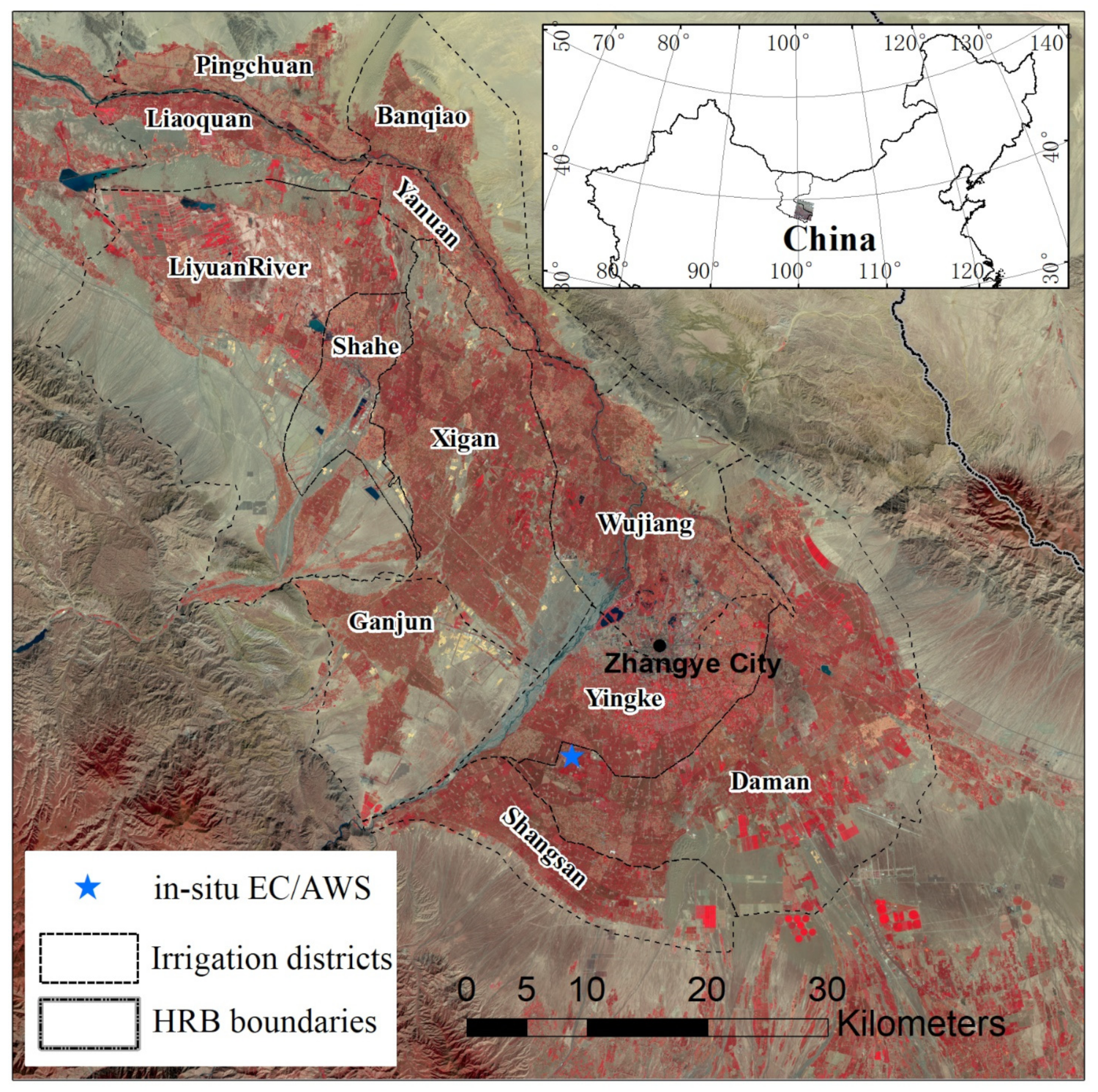
2.1. Study Area

The Heihe River Basin (HRB) (37.65°–42.71° N, 97.05°–102.12° E), with an area of approximately 143,300 square kilometers, is the second-largest endorheic basin in Northwest China. The HRB includes upstream, midstream, and downstream areas. Multi-element, multi-scale, and distributed and incorporated satellite-airborne–ground-based observation networks have been established in the region, including the Watershed Allied Telemetry Experimental Research (WATER) experiment (2007–2011) [51] and the Heihe Watershed Allied Telemetry Experimental Research (HiWATER) experiment (2012–2015) [52,53,54,55]. The average altitude of the Zhangye oasis, which belongs to the typical temperate continental arid climate, is about 1770 m. The average annual temperature is 7.3 °C, the average annual relative humidity is 52%, the main wind direction is northwesterly, the average annual precipitation is 130.4 mm, and the average annual evaporation is 2003 mm (small evaporation pan observation value).

Figure 1 shows the area of interest, which is located in the midstream oasis area of the HRB. Oasis cultivation is located along the Heihe River and surrounded by the Gobi Desert. This agricultural area covers 18 irrigation districts and more than 4000 pumping wells. The study area contains 12 of these irrigation districts (Daman, Shangsan, Ganjun, Yingke, Xigan, Wujiang, Liyuan River, Shahe, Liaoquan, Yanuan, Banqiao, and Pingchuan; Figure 1). In 2012, summer maize was mainly planted in the oasis area. The soil texture of the oasis is mainly pink loam soil. Irrigation of the farmland is mainly channel irrigation. The irrigation water is from the nearby Heihe River using traditional flood irrigation during growth seasons.

2.2. Multi-Platform Satellite Remote Sensing Data

The multi-platform remote sensing data of Terra and Landsat satellites with different spatial and temporal resolutions are listed in

Table 1. Information of multi-platform satellite remote sensing data.

Sensor	Data Name	Start Date	End Date	Spatial Resolution	Temporal Resolution	Location
-	All-weather LST (AWLST)	1 January 2010	31 December 2016	1000 m	Daily	HRB
MODIS	MOD11A1			1000 m	Daily	H25V5
	MCD43A3			500 m	Daily
	MOD13Q1			250 m	16 days
Landsat-5	TM			30/120 m	16 days	P133R033
Landsat-7	ETM+			30/60 m	16 days

. The daily land surface temperature (LST) level 3 product (MOD11A1) is from the MODIS sensor of the Terra satellite at version 6, which was generated based on the generalized split-window algorithm (GSWA) and has an average 1000 m spatial resolution. This product was validated with an accuracy of 0.6–2.6 K for bare soil land [56].

The other MODIS products used include the albedo level 3 product (MCD43A3) at 500 m and the 16-day normalized differential vegetation index (NDVI) level 3 product (MOD13Q1) with 250 m resolution. These MODIS products for the study area from 2010 to 2016 were acquired from the Land Processes Distributed Active Archive Center (LP DAAC, https://lpdaac.usgs.gov/ accessed on 6 April 2021). The all-weather LST product was obtained by integrating the MODIS LST product with the AMSR-E/AMSR2 bright temperature product, as detailed in Zhang et al. [57], and it can be downloaded from the National Tibetan Plateau Data Center (TPDC) (https://data.tpdc.ac.cn/en/ or https://data.tpdc.ac.cn/zh-hans/ accessed on 6 April 2021) (Table 1).

The Landsat data with cloud cover below 15% from 2010 to 2016 were acquired from the USGS (https://landsat.usgs.gov/ accessed on 6 April 2021) to provide high-resolution information about the LST, albedo, NDVI, and emissivity for quantitative remote sensing. These shortwave reflectance bands and the thermal bands of Landsat data were calibrated and corrected, separately, with the QUAC [58] of the ENVI and the Atmospheric Correction Parameter Calculator [59] from NASA (https://atmcorr.gsfc.nasa.gov/ accessed on 6 April 2021). These model input variables (LST, fractional vegetation cover (FVC), NDVI, emissivity, leaf area index (LAI), and canopy height (HC)) for the ET and GPP models were generated at higher spatial (100 m) and temporal (daily) resolution after fusing the MODIS and Landsat data (Table 1).

2.3. Ground Measurements

The EC data were used to validate the revised SEBS and MODIS GPP models from the TPDC website (https://data.tpdc.ac.cn/en/ or https://data.tpdc.ac.cn/zh-hans/ accessed on 6 April 2021). The EC measurements of turbulent and CO₂ fluxes at 10 Hz frequency from the Daman superstation site were processed in the midstream of the HRB (Figure 1). The latent heat flux (LE) of continuous 30 min periods in one day was calculated for the daily ET. To fill gaps for the temporal continuous daily ET, a nonlinear regression method was adopted based on the 30 min LE and net radiation (R_n) data [60]. However, when there was a loss of more than 50% in one day, the daily ET was abandoned, and the missing data were interpolated according to the relationship between the daily LE and the daily R_n of other days. Liu et al. [49,55] and Ma et al. [61] provide more details on the in situ measurements and observation data preprocessing.

For the daily GPP, the EC systems used directly measure the net ecosystem exchange (NEE) rather than GPP. Thus, GPP is the sum of the NEE and daytime respiration (R_dt):

GPP = R_dt − NEE_dt,

(1)

where NEE_dt is daytime NEE. As plants do not photosynthesize at night, nighttime NEE (NEE_nt) represents nighttime respiration (R_nt). The effects of temperature on NEE_nt were described using the following nonlinear regression method [62,63]:

NEE_nt = a₀×EXP(b₀×T_a),

(2)

where T_a is nighttime air temperature. The coefficients a₀ and b₀ were determined based on NEE_nt and the air temperature was from nonlinear optimization. Thus, R_dt can be calculated by extrapolating Equation (2) in conjunction with the daytime temperature.

In addition, because the CO₂ flux can be underestimated using the EC system for nonturbulent conditions [64], the data included in this study were removed with a friction velocity of more than 0.15 m/s. Nonlinear regression between the measured fluxes and environmental factors was used to fill missing data gaps using a moving window [65,66]. The daily GPP was synthesized based on half-hours. When more than 20% of a day’s data was missing, it was indicated as a missing day. The daily GPP values were calculated using a shallow neural network with meteorological variables. Then, the annual values of the GPP were determined by summing all the daily GPP values.

The following meteorological data were collected from the Daman superstation: air temperature, wind speed, pressure, relative humidity, rain, soil temperature and moisture profiles, radiation, and surface soil heat flux. These data were measured by constructing in situ stations at intervals of 10 min [61].

2.4. Meteorological Forcing Data

For regional estimations of ET, GPP, and WUE, the input datasets for the spatial meteorological variables mainly consisted of air temperature, wind speed, humidity, pressure, and downward shortwave radiation from the China Meteorological Forcing Dataset (CMFD) [67,68,69]. The CMFD was made by blending the remote sensing products, the reanalyzed dataset, and observation data from weather stations with high temporal and spatial resolutions (3 h and 0.1°). The evaluated uncertainty for various meteorological factors was based on independent site data and shows that the dataset is more accurate over China than the Global Land Data Assimilation System (GLDAS) dataset, which is widely used throughout the world.

Detailed information on the CMFD dataset is available at https://data.tpdc.ac.cn/en/ or https://data.tpdc.ac.cn/zh-hans/ accessed on 6 April 2021. To more accurately estimate ET and GPP in the study area at high spatiotemporal resolution, it was necessary to match the meteorological variables with remote sensing images at 100 m spatial resolution. The bilinear resampling method was used to interpolate these meteorological variables, and then they were averaged to obtain the daily value. Then, to match the remotely sensed surface variables, the CMFD-derived variables were downscaled to 100 m spatial resolution with regression kriging (RK) [61,70,71].

3. Methodology

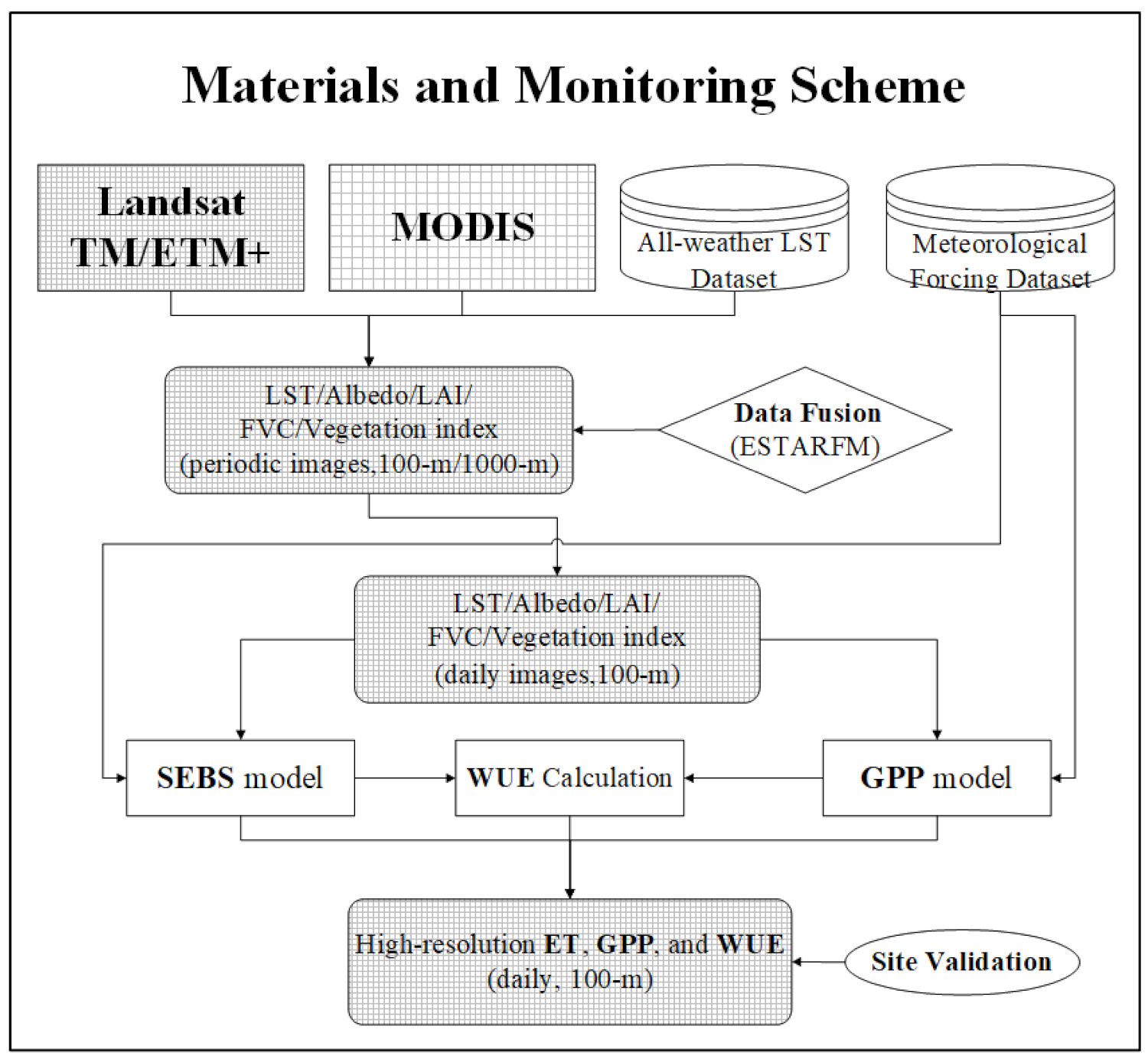
3.1. Workflow for Generating High-Resolution ET, GPP, and WUE

The high-resolution ET, GPP, and WUE processing flow in this study is diagrammed schematically in Figure 2. Here, land surface variables (AWLST, NDVI, and albedo) have been fused with periodic Landsat images at 100 m resolution and MODIS images at 1000 m resolution retrievals using a spatial and temporal fusion of multi-source remote sensing data to create ET, GPP, and WUE with both high temporal (daily) and spatial (100 m) resolution using remote sensing models.

3.2. Models

3.2.1. ET Model

The SEBS model, a classical single-source surface energy balance approach with a clear physical mechanism, was used to estimate turbulent heat fluxes and daily ET through a combination of satellite remote sensing data and meteorological data [72]. The calculation of sensible heat flux (H) was used to establish the following nonlinear equations and solve them iteratively based on the Monin–Obukhov similarity theory (MOST) and the bulk transport equation:

$$H=k{u}_{\ast }\rho C_p({\theta }_0-{\theta }_{\mathrm{a}}){\left[\ln \left(\frac{z-d_0}{z_{0h}}\right)-{\psi }_h\left(\frac{z-d_0}{L}\right)+{\psi }_h\left(\frac{z_{0h}}{L}\right)\right]}^{-1},$$

(3)

$$u=\frac{u_{*}}{k}\left[\ln \left(\frac{z-d_0}{z_{0m}}\right)-{\Psi }_m\left(\frac{z-d_0}{L}\right)+{\Psi }_m\left(\frac{z_{0m}}{L}\right)\right],$$

(4)

$$L=-\frac{\rho C_p{u}_{*}^3{\theta }_v}{kgH},$$

(5)

where z is the reference height; u_* is the friction velocity; k is the von Kármán constant; ρ is the density of the air; C_p is the specific heat of the air at constant pressure; u is the wind speed; d₀ is the zero-plane displacement height; g is acceleration due to gravity; θ_v is the potential virtual temperature; z_0h and z_0m are the roughness heights for the heat and momentum transfer, respectively; Ψ_h and Ψ_m are the stability correction functions for the sensible heat and momentum transfer [73,74,75], respectively; and L is the Monin–Obukhov length.

In this study, the optimized parameterization scheme of the SEBS model was adopted [61], and the lack of optical remote sensing data was overcome by using the AWLST data products due to frequent cloud contamination and other poor atmospheric conditions [57]. Instantaneous LE/ET was then calculated from instantaneous net radiation (R_n), H, and surface soil heat flux (G₀) by substituting in the energy balance. On this basis, the scaled-up time-scale method of instantaneous to daily surface evapotranspiration (the constant solar radiation ratio, SolRad [76]) was used to calculate daily surface evapotranspiration.

3.2.2. GPP Model

The MODIS land product algorithm (MOD17A2) [77] for daily GPP is calculated as:

$$GPP=\epsilon \times APAR = \epsilon \times IPAR\times FPAR,$$

(6)

$$APAR=IPAR\times FPAR,$$

(7)

$$IPAR=SWRad\times 0.45,$$

(8)

$$FPAR=NDVI\times 1.24-0.168,$$

(9)

where APAR is the absorbed photosynthetically active radiation. IPAR can be estimated from the incident shortwave radiation (SWRad) using Equation (8), and FPAR is the fraction of photosynthetically active radiation. Here, FPAR from satellite-derived data in Equation (9) is used instead of the direct quantization of spectral vegetation indexes, such as the NDVI in the MODIS algorithm [78]. The ε is a conversion factor, which varies widely for different vegetation types [79,80,81]. It is calculated as

$$\epsilon ={\epsilon }_{\max }\times T_{\min Scalar}\times VP{D}_{Scalar} ,$$

(10)

where ε_max is the maximum conversion factor, obtained from the Biome Property Look-Up Table (BPLUT) parameters [77], and T_minScalar and VPD_Scalar are the linear attenuation scalars from the daily minimum temperature (T_min) and vapor pressure deficit (VPD), respectively.

3.2.3. WUE Calculation

The ecosystem water-use efficiency (WUE) is calculated as daily/monthly/annual GPP divided by daily/monthly/annual ET.

3.3. Multi-Source Remote Sensing Data Fusion

The enhanced spatial and temporal adaptive reflectance fusion model (ESTARFM), initially developed by Zhu et al. [82] for downscaling reflectance using MODIS and Landsat reflectance band data, has been used effectively to prepare surface biophysical parameters with high spatial and temporal resolution [83,84,85,86]. ESTARFM applies a linear endmember and mixture pixel spectral mode at date t_o and t_p:

$$\begin{array}{l}{M}_{\mathrm{o}}={\displaystyle \sum _{i=1}^N{f}_i}\left(\frac{1}{a}{L}_{i\mathrm{o}}-\frac{b}{a}\right)+\epsilon \\ M_p={\displaystyle \sum _{i=1}^N{f}_i}\left(\frac{1}{a}{L}_{ip}-\frac{b}{a}\right)+\epsilon \end{array}$$

(11)

where M_o and M_p are the reflectance of mixed MODIS pixels at t_o and t_p, respectively; f_i is the fraction of the ith endmember; L_io and L_ip are the reflectance of the ith endmember obtained from Landsat images at t_o and t_p, respectively; N is the total number of endmembers; ε is the residual error; and a and b are the coefficients.

It is assumed that the proportion and change rate of endmember reflectance are steady. A simple linear regression model was used to obtain the conversion coefficient. The geographic and spectral distance weights were considered by using the neighboring pixel information within a moving window. Thus, the predicted reflectance (R) of high-spatial-resolution pixel at t_p can be described as:

$$L_p\left(x_{w/2},y_{w/2},R\right)=L_o\left(x_{w/2},y_{w/2},R\right)+{\displaystyle \sum _{i=1}^S{W}_i{V}_i(M_p(x_i,y_i,R)-M_o(x_i,y_i,R))},$$

(12)

where S is the number of similar pixels; W_i is the weight, determined by the distances of similar pixels and the spectral similarity from Landsat and MODIS data; and V_i is the conversion coefficient, which is computed with a simple linear regression model based on similar pixels.

Finally, the temporal weighting method, based on changes of the coarse spatial resolution reflectance between time t_o (o = m or n) and prediction time t_p, was used to further improve the prediction accuracy of the algorithm. A more detailed description of ESTARFM is in Zhu et al. [82]. Here, ESTARFM was applied to produce land surface variables, such as AWLST (daily), NDVI (16 day), and albedo (daily), at a spatial resolution of 100 m using multi-platform remote sensing data described in Section 2.1. Previous studies have reported that direct fusion of surface physical parameters (e.g., NDVI) is very effective [85,86].

3.4. Footprint of Flux Source Area

Several verifications use the latitude and longitude of the observation instrument site to determine the corresponding pixels for obtaining estimations of the remote sensing data and comparing with EC measurements. If the observation sensor is installed at a certain height, the underlying surface is flat and there is no flat flow effect. Thus, the measured value reflects the average condition of the area where the site is located, and the measured and estimated values of the remote sensing model have the same regional representativeness. However, such environmental conditions are difficult to satisfy.

The observed values can only reflect the information for a specific underlying surface or a portion therein, but cannot represent the average value of the pixel space range corresponding to the observation site. Therefore, directly verifying the pixel value of the station where the instrument is located using the measurements has the problem of mismatched spatial representation range between the measured ET/GPP value on the ground and the estimated value from remote sensing. Thus, a Eulerian analytic flux footprint model that can determine the measurement range of ground instruments to select the corresponding pixels more accurately was used to verify the remote sensing estimations [87].

The image pixels of ET/GPP/WUE estimations within the EC flux source area were extracted for validation [88,89]. The specific operation was as follows. First, a relative weight distribution map of the source area was obtained using the footprint. Then, the footprint distribution map was superimposed onto the corresponding position of the remote sensing image. The weighted calculation of the pixels in the source region then provided the remote sensing estimation results with the same spatial representation range as the ground flux observation values.

4. Results and Discussion

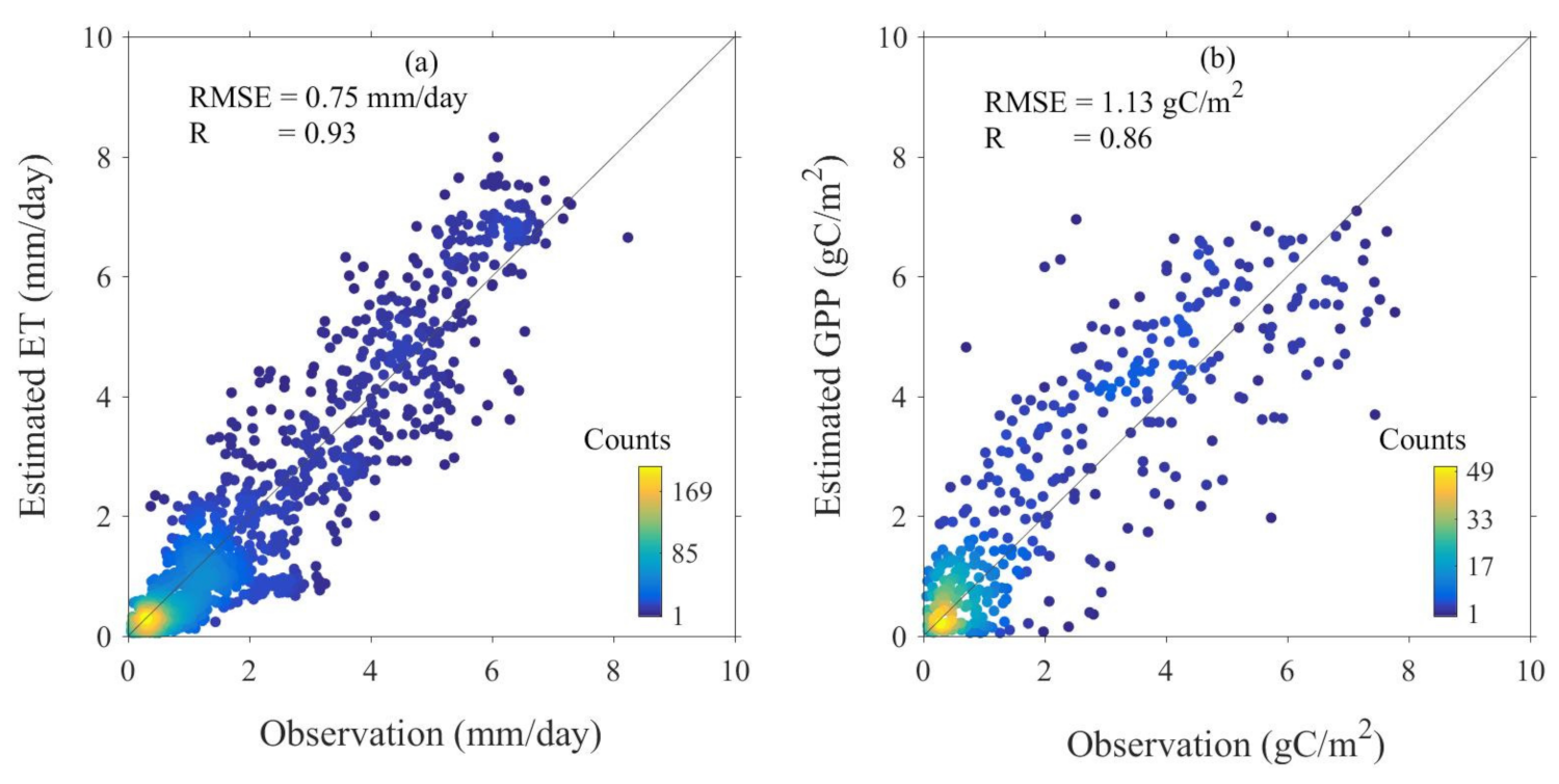
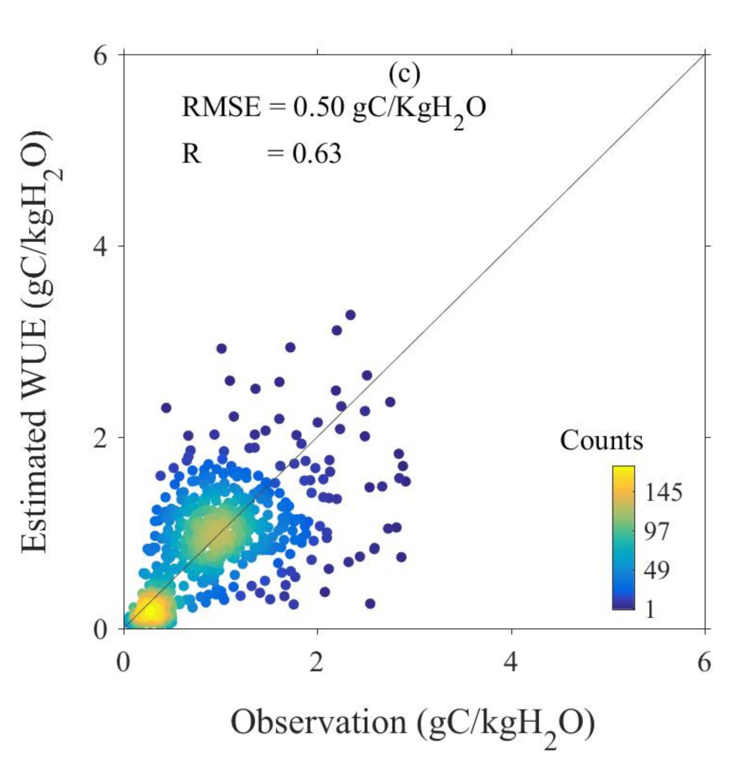
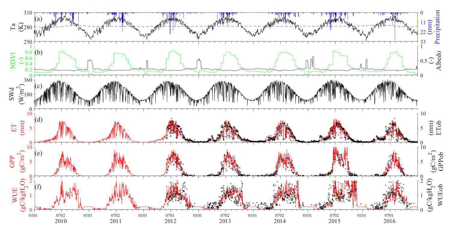
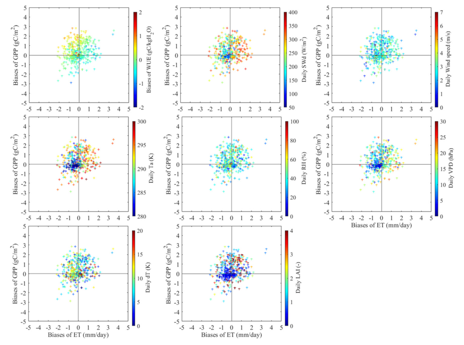
4.1. Assessment of Daily ET, GPP, and WUE at Footprint Scale

Overall, the validation results indicate that daily ET, GPP, and WUE can be reliably produced over the midstream oasis agricultural areas in the HRB for the considered multi-year study period (ET: NSE 0.84, MAPE 26.59%, RMSE 0.75 mm/day, R = 0.93; GPP: NSE 0.70, MAPE 36.26%, RMSE 1.13 gC/m², R = 0.86; WUE: NSE 0.28, MAPE 39.83%, RMSE 0.50 gC/kgH₂O, R = 0.63) (

Table 2. Statistics for model validations to estimate daily ET, GPP, and WUE for cropland (maize) cover types from Daman superstation in oasis midstream area. NSE, Nash–Sutcliffe efficiency coefficient; MBE, mean bias error; RMSE, root mean square error; MAPE, mean absolute percent error; R, correlation coefficient.

Type	Site	Variables	NSE	MBE	MAPE	RMSE	R
Cropland (maize)	DMS	Unit	-	mm/day	%	mm/day	-
		Daily ET	0.84	−0.06	26.59	0.75	0.93
		Unit	-	gC/m2	%	gC/m2	-
		Daily GPP	0.70	0.21	36.62	1.13	0.86
		Unit	-	gC/kgH2O	%	gC/kgH2O	-
		Daily WUE	0.28	−0.05	39.83	0.50	0.63

). We integrated the ET, GPP, and WUE estimates at the 100 m scale to the same spatial representation as the EC measurements based on the EC flux source area. We then contrasted the integrated daily ET, daily GPP, and daily WUE estimates with the EC measurements at the Daman superstation (DMS) (Figure 3a–c). The results show that the daily estimated value is in good agreement with the EC measurements (Figure 3). The best performance was for estimated daily ET from the SEBS model. This is evidenced by the high NSE (>0.84), low RMSE (<0.75 mm/day), and low bias, as shown in Table 2. The errors were significantly lower than those reported by Cammalleri et al. [90,91], with an RMSE ranging from 1.11 to 1.81 mm/day and an approximate MAPE from 20.8 to 26.6% for the irrigated field. The second best was for the estimated daily GPP using the MODIS GPP product algorithm (NSE 0.70), and the third best was for the estimated daily WUE (NSE 0.28).

As WUE was calculated based on the ratio of GPP to ET, which have similar magnitudes, WUE exhibited relatively large fluctuations and likely contained significant uncertainties. When the average ET was small, small perturbations also had a large impact on WUE, which resulted in reduced accuracy, such as when it was measured outside of the growing season, as shown in Figure 4. Therefore, the MAPE of WUE was greater than that of ET and GPP. Based on the progress of research on WUE, Zhou et al. [92,93] proposed a new calculation method for potential WUE (uWUE = GPP·VPD^0.5/ET) by considering the nonlinear effect of VPD. Because it takes into account the response of stomatal conductance to VPD, it can better reflect the physiological regulation of the water–carbon exchange in plants, and has better stability and accuracy. Therefore, new methods could be considered to reduce the uncertainty of WUE in future studies.

The accuracy of the available meteorological datasets showed marked differences both spatially and temporally [67]. Uncertainties related to the use of coarse spatial resolution meteorological elements and multi-satellite remote sensing data can have different degrees of influence on the results [94]. Here, meteorological forcing data, such as temperature, relative humidity, wind speed, and radiation, are required as SEBS and GPP model inputs, which is bound to cause errors in the estimation results. However, it is very difficult to obtain large-scale and fine-resolution meteorological data at present, and new techniques for observing meteorological variables could provide a solution in the future. In addition, several factors reduce the prediction quality of surface parameters with ESTARFM, such as temporal variance, cloud coverage, spatial heterogeneity, and view angle effects.

Comparing the observed ET or GPP with the estimated WUE based on a dataset from one site could bring uncertainties as a result of differences in the observation orientation and environmental conditions at a given in situ station [95]. In addition to the inherent uncertainties in the validation data of EC and GPP, the mismatched spatial locations between estimated ET, GPP, and EC measurements will also affect the accuracy [88,89].

Figure 4 shows the time series data of estimated and observed daily ET, GPP, and WUE and the response of temporal variations in daily temperature (Ta), daily precipitation, daily incident shortwave radiation (SWd), daily albedo, and NDVI (16 days) under cropland cover conditions in the midstream oasis area of the HRB during the multi-year study period (2010–2016). The daily temporal variations in estimated and observed values showed similar patterns in midstream oasis agricultural areas over the study period, especially during the growth seasons. Of the three, estimated and observed WUE performed the worst.

The temporal variations in daily ET, GPP, and WUE indicate some key factors when determining ET, GPP, and WUE, including Ta, precipitation, SWd, albedo, and NDVI (Figure 4a–c). When the daily temperature was below 5 °C, the daily ET was relatively small and the daily GPP and WUE were near 0. Thus, warmer temperature mainly determined daily ET, GPP, and WUE over the midstream oasis area of the HRB. Although precipitation did not solely determine daily ET, GPP, and WUE, their peak durations were a direct response to rainfall/cloudy events in the growing season. The duration of peak stages was influenced by the time distribution characteristics of precipitation for the year. For example, in 2011 and 2016, the profiles for ET, GPP, and WUE were significantly abnormal due to the concentrated and relatively low rainfall (Figure 4a,d,f). In addition, Figure 4b shows that the seasonal variations of NDVI were basically consistent with estimated ET, GPP, and WUE.

In midstream oasis areas with relatively low precipitation, the rain gauge-observed precipitation (TE525MM, Texas Electric, USA) at the DMS (Figure 4a) also showed high daily ET (5–8 mm/day), GPP (5–8 gC/m²), and WUE (1–1.5 gC/kgH₂O) during the growing season. This is because the midstream oasis area has irrigation water supplied from the surface and groundwater (Figure 4d,f).

In general, high GPP values correspond directly to high ET values, and vice versa, and the trends of WUE over the midstream oasis area of the HRB were similar but larger discrepancies were seen (Figure 4). There were large differences in the early and late periods of the growth season and periods of precipitation. The estimated and observed ET and GPP values increased rapidly in the initial stage of the growth season and reached maxima in the middle of July as the plants matured, before declining gradually in late August through the subsequent senescent stage. As WUE is a ratio using GPP and ET, their results directly determine WUE estimations, particularly its magnitude. Considering the high coupling between photosynthesis and transpiration, the remote sensing-based models were mostly consistent in their estimates of GPP and ET biases, which helps to reduce the bias in WUE estimates. However, there were also larger inconsistencies between GPP and ET, as shown in Figure 5. These large inconsistent biases were amplified in the WUE estimation, resulting in poorer estimation results. Although the biases are sometimes small, there will still be a large WUE bias due to the lower ET value and low magnitude at this time. At this point, it is due to the limitations of the WUE model itself. The anomaly of the carbon–water coupling process in the oasis ecosystem found in this study was consistent with previous reports [96].

Overall, the estimation models captured changes in ET, GPP, and WUE following weather conditions (precipitation) and anthropogenic activities (irrigation or fertilizer application), which can be fully caught in the changes in crop growth and phenology using multi-source remote sensing data.

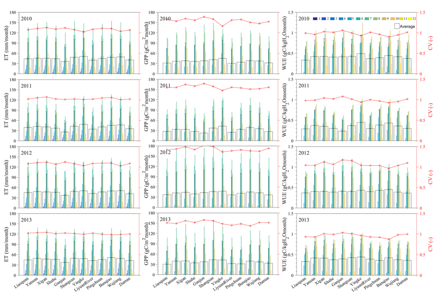
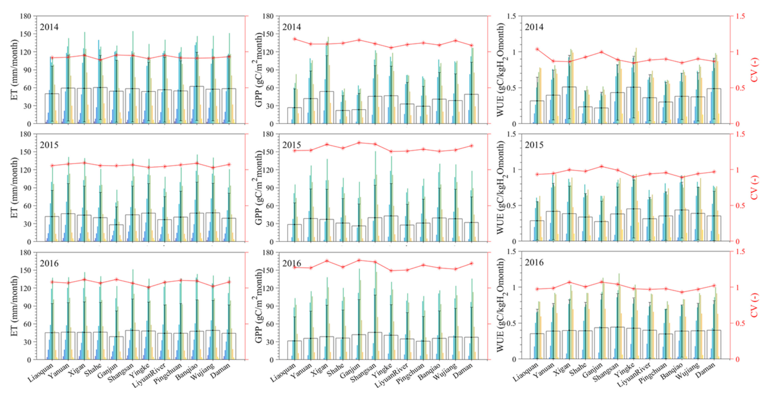
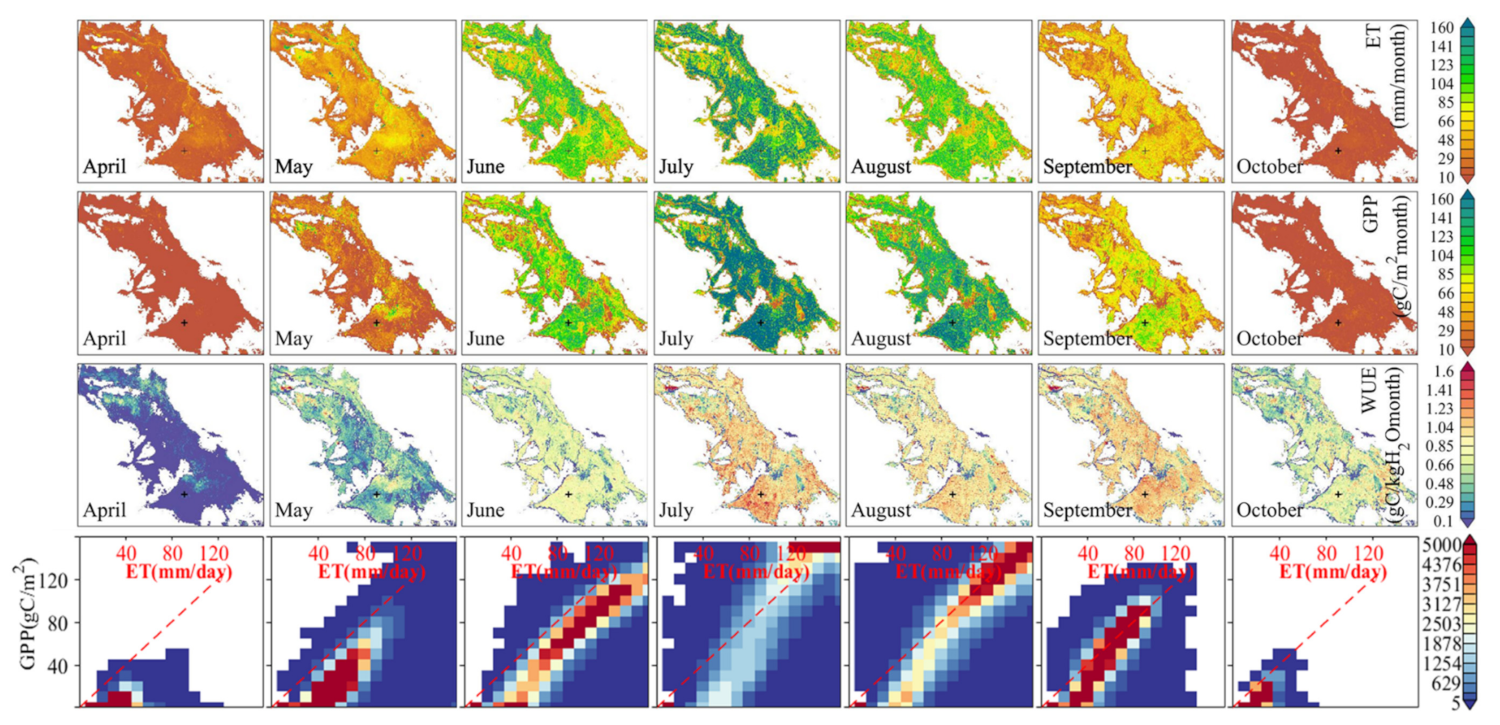
4.2. Variations in Monthly ET, GPP, and WUE for 12 Irrigation Districts

To quantitatively understand oasis agricultural water consumption, cropland biomass production, and water product between irrigation districts, histograms of the average monthly ET for the Daman, Shangsan, Ganjun, Yingke, Xigan, Wujiang, Liyuan River, Shahe, Liaoquan, Yanuan, Banqiao, and Pingchuan districts, which represent the oasis agricultural areas in the identified geographic locations, are plotted for all months from 2010 to 2016 (Figure 6). The monthly regional ET from 2010 to 2016 is plotted in Figure 6 (first column), with the seasonal variations of each irrigation district showing a unimodal curve with a peak in July.

From June to August in all years, the average monthly regional ET in each irrigated area generally changed directly from 120 to 150 mm; however, there were certain exceptions. For example, in 2011 and 2015, the maximum monthly regional ET value in the Ganjun irrigation district was approximately 75 mm. On the other hand, the maximum value in the Shangsan and Banqiao districts in 2010, Shangsan and Xigan and Daman districts in 2014, and Shangsan irrigation district in 2016 exceeded 150 mm. The seasonal patterns of ET in the oasis agricultural area in the arid and semi-arid region of Northwest China are distinct from those of moist areas of the same latitude in the North China Plain (NCP) [97]. This is because single crops account for the majority of the former, and double crops in rotation account for the majority of the latter.

The monthly regional patterns (seasonal variations) in GPP and WUE have a strong resemblance to ET for different irrigation districts, as shown in Figure 6 (second and third columns). However, the monthly spatial variation patterns are different from the amplitude changes and CV statistical indicators for the different irrigation districts (Figure 6, red stars). At the irrigated area scale, ET had the smallest spatial variation, GPP had the largest spatial variability, and WUE was in the middle. Numerous studies reported that the primary irrigation method in midstream oasis agricultural areas has always been flood irrigation from the surface and groundwater [61]. In other words, each irrigated area has a sufficient water supply during the growing season.

In addition, the crop for the entire oasis is mostly field corn. Therefore, the differences in ET for each irrigated area are relatively small. However, in addition to the influence of irrigation, other anthropogenic activities, such as changing the amount of fertilizer applied and renewing plant varieties, also greatly affect the changes in GPP for each irrigated district. Previous studies in the NCP have proved this [98,99]. As a result, GPP showed stronger variability in years with both large (2011 and 2015) and small (2010 and 2013) ET seasonal changes among the 12 irrigation districts.

The spatiotemporal variability of WUE is jointly affected by ET and GPP. In general, a higher monthly ET also means a greater GPP, which gives a higher WUE for each irrigation district (Figure 6). More importantly, at the monthly scale, WUE values of the oasis croplands the early (May) and late (June) growing seasons are close to the mid-growing season (July and August) (Figure 6, third column). The early WUE was slightly lower because ET added in the early stage was significantly faster than GPP, while ET added in the later stage showed a synchronous decrease (nearly linear), which is confirmed in the following, with bivariate histograms between monthly ET and GPP. This is an important finding and indicates the factors that describe monthly WUE and water-saving irrigation time allocation schemes in midstream oasis agricultural areas.

A significant lag in the early stages in WUE was found for irrigation district croplands, which may be attributable to the significant increase in early ET without obvious changes in early GPP over the entire oasis agricultural area. In the same study area, Ma et al. [61] also reported that the depth of irrigation was approximately 690 mm for all irrigation districts in 2012. This signifies monthly irrigation of at least 57.5 mm, which is significantly higher than the monthly ET for the 12 irrigation districts (Figure 6, black box).

These differences reflect the water-saving irrigation and specific implementation time point based on the study recommendations at the beginning of the growing season. That is, this period should be more economical than the current irrigation water-use period. Further studies may determine the WUE of irrigated farmland and the allocation mechanism for irrigation water resources that dictate the importance of these factors.

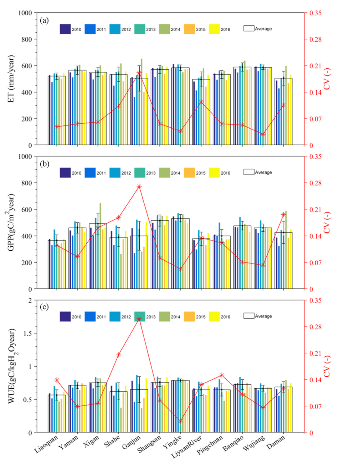
4.3. Spatiotemporal Variations of Multi-Year ET, GPP, and WUE for 12 Irrigation Districts

The temporal dynamics of the multi-year ET, GPP, and WUE in each irrigation district from 2010 to 2016 are shown in Figure 7 (histograms represent the average of oasis agricultural areas with the geographical location identified by the 12 irrigation districts). The multi-year regional average values (Figure 7, black box) and the multi-year temporal dynamics coefficient of variation (CV) characteristics (Figure 7, red stars) of GPP, ET, and WUE for each irrigated district were similar in midstream oasis agricultural areas.

The highest mean multi-year ET (580 mm) was found for the Banqiao, Wujiang, and Yingke districts, and the lowest mean (500 mm), for the Liyuan River district (Figure 7a). An analysis of annual variations (σ_ann and CV) indicates the annual ET of Ganjun had the largest variations from 2010 to 2016 (σ_ann 96 mm, CV 0.19) and that of Wujiang had the smallest variations (σ_ann 16 mm, CV 0.03). No significant temporal variation trend in annual ET was found for the seven-year study period (2010–2016) over the midstream oasis.

The highest mean multi-year GPP (530 gC/m²year) was found for the Yingke irrigation district, and the lowest (370 gC/m²year) for Liaoquan (Figure 7b). The annual variations (σ_ann, CV) indicated that the annual GPP of Ganjun was the largest (σ_ann 108 gC/m², CV 0.27) and that of Wujiang was the smallest (σ_ann 28 gC/m², CV 0.06). No significant temporal variation trend in annual GPP was found for the study period (2010–2016).

The results show that on an annual scale, the oasis croplands of the irrigation districts with higher ET also had higher GPP, which ultimately produces larger WUE. However, while the Wujiang irrigation district had higher annual ET and GPP than the Daman district, its WUE was lower (Figure 7c). WUE exhibited relatively small interannual variability. For example, WUE for Yingke and Wujiang was basically the same over all years.

In addition, the highest mean multi-year WUE (0.80 gC/kgH₂Oyear) was found for Yingke and the lowest (0.58 gC/kgH₂Oyear) for Liaoquan (Figure 7c). The annual variations (σ_ann, CV) indicate that the annual WUE of Ganjun was the largest (σ_ann 0.19 gC/kgH₂O, CV 0.30) and that of Yingke was the smallest (σ_ann 0.02 gC/kgH₂O, CV 0.03). In a previous study, Xiao et al. [43] showed mean annual WUE values from 0.5 to 1.0 gC/kgH₂O for vegetation (including grassland and cropland) across various ecosystem types in China.

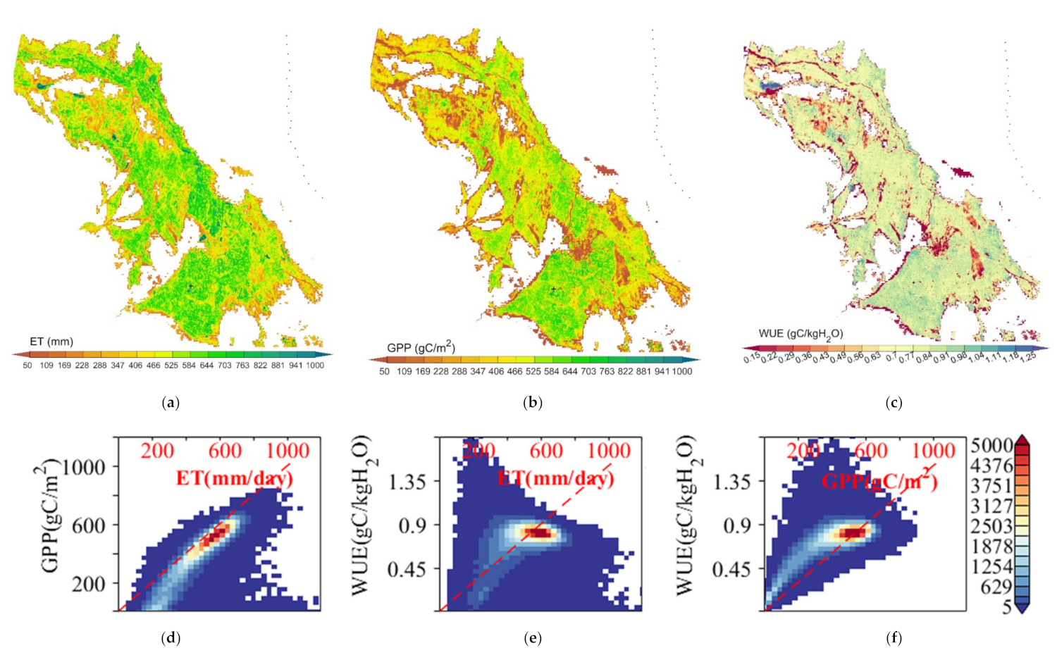
4.4. Spatial Characteristics of ET, GPP, and WUE for Midstream Oasis Agricultural Areas

Spatial patterns at the fine-grain scale for monthly and yearly ET, GPP, and WUE over the midstream oasis of the HRB during the growing season (April to October) are variable and complex and based on different net irrigation water distributions, cropping patterns, and seasonal weather conditions. Remote sensing and spatial-statistical mapping give the spatial distributions of monthly and yearly ET, GPP, and WUE from the modeled daily values through the entire midstream oasis area from April to October, which are shown to reveal temporal changes at the regional scale. The data from 2013 were selected as an example to map the spatial characteristic information (Figure 8 and Figure 9).

The monthly ET and GPP maps using remote sensing models (Figure 8, rows 1 and 2) show that the spatial distribution pattern of ET and GPP changed from April to October in 2013. While the monthly ET and GPP had minor responses in the early growth season (April and May), there were slightly larger changes for ET in the riverway and GPP in the wheat-growing areas of the oasis, for example, around the southern part of Zhangye City. In June, monthly ET and GPP values increased significantly for croplands in the midstream oasis. These larger values are associated with maize seeding in late May, as the vegetation begins to germinate and turn green later in the spring, which is followed by irrigation and solar radiation enhancement. In July and August, crop water consumption (i.e., ET) increases rapidly as the vegetation growth rate and biomass (i.e., GPP) accumulation rate is the highest in these two months. Late in the growth season, the oasis crops mature, and frost begins to occur. Thus, there is a significant decrease in ET and GPP for September. In October, the solar radiation decreases significantly, and ET and GPP are further reduced.

As shown in Figure 8, row 3, the spatial characteristics of monthly WUE are significantly different from ET and GPP from April to October. In April and May, the monthly WUE throughout the entire oasis area was generally low. In June and October, WUE was generally around 0.80 gC/kgH₂O, while in July to September, during the vigorous growth of oasis crops, monthly WUE remained at around 1.25 gC/kgH₂O. This phenomenon can be seen more intuitively from the bivariate histograms between monthly ET and GPP. This behavior can be explained to some extent. In the spring in arid areas (early growing season), enhanced radiation and irrigation activities lead to rapidly increasing water consumption (ET) of the oasis, and there is more soil evaporation at this time. As oasis crops are in the sowing and seedling stage at this time, there is less transpiration and a slow biomass increase (Figure 8, row 4, April and May). From July to October, ET and GPP were relatively small, and WUE was nearly stable at higher values ranging from 1.00 to 1.35 gC/kgH₂O. This is because the synchronization of monthly ET and GPP decreased linearly during this period (Figure 8, row 4, June to October). This synchronous linear decrease may be because the vegetation cover in the oasis area inhibits soil evaporation to an extent, even when the vegetation declines. In the case of insufficient agricultural water resources, more attention should be paid to the temporal variation of water use during the growing season in order to achieve a transformation from traditional high-yield irrigation to water-saving and high-quality irrigation [100]. However, in-depth investigation and research work are still required to determine the feasibility of this approach.

Regional yearly ET, GPP, and WUE, as derived from remote sensing methods, can illustrate their spatial variations in the oasis (Figure 9a–c). Annual ET, GPP, and WUE varied from 300 to 700 mm (accounting for 90%), 200 to 650 gC/m² (accounting for 90%), and 0.5 to 1.0 gC/kgH₂O (accounting for 95%), respectively, over the entire irrigation agriculture district under different cropping patterns and water resource conditions. The highest ET was observed for reservoirs and ponds and the watercourses of the Heihe River within the oasis, while GPP was the lowest. Due to the existence of roads and residential areas, and shortages in vegetation cover and water supplies inside the oasis, annual ET and GPP were notably lower. Thus, higher ET and GPP were obtained in the cropping oasis areas. Annual ET, GPP, and WUE in 2011 and 2014 were significantly smaller than the multi-year averages of 580 mm, 500 gC/m², and 0.86 gC/kgH₂O, respectively. The characteristics of their spatial distributions did not change significantly over the seven-year study period (2010–2016), except for the eastern part of the oasis (results of that mapping not shown here). Land cover changes greatly affected ET and GPP patterns, and much higher ET and GPP values were observed at fine spatial resolution under the eastern part of the oasis, where they reached their highest levels. This fine-grained estimation of increasing annual variation indicates the expansion of the oasis agriculture area and/or human disturbances.

There was a linear relationship between annual oasis cropland ET and GPP. When ET was greater than 400 mm, it was slightly greater than the GPP value (Figure 9d). However, annual WUE presented a nonlinear relationship with ET and GPP (Figure 9e,f). When annual ET and GPP were greater than 550 mm and 500 gC/m², annual oasis cropland WUE had strong invariability and was maintained at approximately 0.85 gC/kgH₂O. This is an important finding and indicates the factors that describe cropland WUE at the annual scale over the irrigation oasis agricultural area of an arid region. When WUE was high (≥0.85 gC/kgH₂O), annual oasis cropland ET was maintained at 500 mm, which means the use of irrigation water should be reduced as much as possible. Generally, the variations and constraint relationships between annual ET, GPP, and WUE in the oasis of an arid area are attributed to changes in the water supply, crop planting patterns, surface cover type, and anthropogenic fertilizer application.

The strong correlation between GPP and ET demonstrates that the carbon and water cycles are a tightly coupled system [101,102]. This is particularly true of our findings in arid oasis croplands (Figure 8 and Figure 9). The direct determinants of the cropland WUE are the GPP and ET. Specifically, the cropland WUE varied depending on the irrigation amount, period, variety, and methods [103,104]. In general, some varieties more easily produce high yield and high WUE under lower irrigation conditions [105,106]. For example, studies have shown that appropriate deficit irrigation will not significantly affect wheat yield but will significantly reduce irrigation water and crop water consumption, which improves the irrigation efficiency and WUE for wheat [107,108], whereas exceeding the suitable irrigation water consumption reduces the WUE [109,110]. In future work, the appropriate deficit irrigation strategies for the water-resources-limited irrigation districts of HRB should be further studied rather than the current flood irrigation in arid ecosystems [100,111,112].

In many regions around the world, cropland WUE is often applied to farmland to relieve the water resource pressure and improve its irrigation management [95]. Thus, water-saving irrigation aimed at maximizing the WUE of crops is regarded as the primary method to address water resource shortages. In Figure 8 row 4, the results of this study show that this was an effective strategy, but the need varies over time and by location. For example, the middle oasis area of the HRB was suitable to reduce soil evaporation based on farmland measures with film mulching in the early growing season, and cropland WUE was improved during this period. However, the increased cropland WUE in many grain planting areas is not necessarily accompanied by a decreased water shortage. This is because, despite the increased WUE, there is an increased planting area, higher crop density, and more water-intensive crops [113]. The decreasing trend of total foodstuff production, as an indicator of groundwater consumption, in terms of water tank capacity around the world, illustrates this phenomenon [114], such as the NCP, Northern India (NI), Southeast Africa (SA), and Tigris–Euphrates River (TER) regions. Therefore, future research should investigate WUE and other indicators to comprehensively reflect irrigation water resource shortages caused by consumption or the differences in the water demand–water diversion allocation schemes and the actual influence of the ecological environment.

Water resource is an important factor to maintain the balance of a green ecosystem. In arid regions, water resource shortages are manifested primarily in the uneven distribution and consumption of water over time and the space between basins [115]. For example, continuous population growth and the large-scale expansion of irrigation agriculture in the midstream regions of HRB have led to an imbalance in the distribution of limited water resources between agricultural water for the midstream of an oasis and ecological water demands for downstream, which has caused serious water resource shortage issues [61]. Moreover, with the increasing demand of water resources, the contradiction of water quota allocation is increasing in the midstream and downstream regions. In irrigation water management, this highlights the importance of improving WUE to cope with water shortages. However, scientific and reasonable water distribution schemes may be more effective for water-limited regions, such as the HRB.

5. Conclusions

Accurate and continuous ET and GPP products with high spatiotemporal resolution are essential for monitoring farmland water consumption and productivity in irrigation oasis agricultural areas in arid regions, which can be derived from multi-source satellite remote sensing data using a data fusion algorithm and remote sensing-based models. The site-level evaluation results with ground observations showed that daily estimated ET, GPP, and WUE had better performance. The daily variations and seasonal and interannual spatial patterns of ET, GPP, and WUE were shown to be reasonable and to reveal fine-grained changes at the 100 m scale among roadways, building areas, riverways, and farmlands with different planting types throughout the oases from 2010 to 2016. This supports our understanding of cropland WUE and improving practices of refined water-saving agricultural management in irrigation oasis agricultural areas. Moreover, the results suggest that the monitoring scheme of the coupled carbon and water cycles using remote sensing-based models (e.g., SEBS and GPP models) enables a water consumption analysis and irrigation management for croplands in other regions. Future work should use satellite data with higher spatial resolution (e.g., Sentry-2) and quantification of WUE at fine scale (e.g., 10 m × 10 m) to optimize the suitability of planting crops under restricted freshwater resources in arid and semi-arid regions.

References

1. Zhang, Y.; Pena-Arancibia, J.L.; McVicar, T.R.; Chiew, F.H.; Vaze, J.; Liu, C.; Lu, X.; Zheng, H.; Wang, Y.; Liu, Y.; et al. Multi-decadal trends in global terrestrial evapotranspiration and its components. Sci. Rep. 2016, 6, 19124. [Google Scholar] [CrossRef] [PubMed] [Green Version]
2. Chen, X.; Su, Z.; Ma, Y.; Yang, K.; Wang, B. Estimation of surface energy fluxes under complex terrain of Mt. Qomolangma over the Tibetan Plateau. Hydrol. Earth Syst. Sci. 2013, 17, 1607–1618. [Google Scholar] [CrossRef] [Green Version]
3. Chen, X.; Su, Z.; Ma, Y.; Liu, S.; Yu, Q.; Xu, Z. Development of a 10-year (2001−2010) 0.1° data set of land-surface energy balance for mainland China. Atmos. Chem. Phys. 2014, 14, 14471–14518. [Google Scholar] [CrossRef] [Green Version]
4. Norman, J.M.; Kustas, W.P.; Humes, K.S. Source approach for estimating soil and vegetation energy fluxes in observations of directional radiometric surface temperature. Agric. For. Meteorol. 1995, 77, 263–293. [Google Scholar] [CrossRef]
5. Kustas, W.P.; Norman, J.M. Evaluation of soil and vegetation heat flux predictions using a simple two-source model with radiometric temperatures for partial canopy cover. Agric. For. Meteorol. 1999, 94, 13–29. [Google Scholar] [CrossRef]
6. Mu, Q.; Zhao, M.; Running, S.W. Improvements to a MODIS global terrestrial evapotranspiration algorithm. Remote Sens. Environ. 2011, 115, 1781–1800. [Google Scholar] [CrossRef]
7. Fisher, J.B.; Tu, K.P.; Baldocchi, D.D. Global estimates of the land–atmosphere water flux based on monthly AVHRR and ISLSCP-II data, validated at 16 FLUXNET sites. Remote Sens. Environ. 2008, 112, 901–919. [Google Scholar] [CrossRef]
8. Yao, Y.; Liang, S.; Cheng, J.; Liu, S.; Fisher, J.B.; Zhang, X.; Jia, K.; Zhao, X.; Qin, Q.; Zhao, B.; et al. MODIS-driven estimation of terrestrial latent heat flux in China based on a modified Priestly-Taylor algorithm. Agric. For. Meteorol. 2013, 171–172, 187–202. [Google Scholar] [CrossRef]
9. Miralles, D.G.; Holmes, T.R.H.; De Jeu, R.A.M.; Gash, J.H.; Meesters, A.G.C.A.; Dolman, A.J. Global land-surface evaporation estimated from satellite-based observations. Hydrol. Earth Syst. Sci. 2011, 15, 453–469. [Google Scholar] [CrossRef] [Green Version]
10. Beer, C.; Reichstein, M.; Tomelleri, E.; Ciais, P.; Jung, M.; Carvalhais, N.; Rödenbeck, C.; Arain, M.A.; Baldocchi, D.; Bonan, G.B.; et al. Terrestrial gross carbon dioxide uptake: Global distribution and covariation with climate. Science 2010, 329, 834–838. [Google Scholar] [CrossRef] [Green Version]
11. Zhang, Y.; Xiao, X.; Wu, X.; Zhou, S.; Zhang, G.; Qin, Y.; Dong, J. A global moderate resolution dataset of gross primary production of vegetation for 2000–2016. Earth Syst. Sci. Data. 2017, 4, 170165. [Google Scholar] [CrossRef] [Green Version]
12. Zhao, J.; Feng, H.; Xu, T.; Xiao, J.; Guerrieri, R.; Liu, S.; Wu, X.; He, X.; He, X. Physiological and environmental control on ecosystem water use efficiency in response to drought across the northern hemisphere. Sci. Total Environ. 2021, 758, 142599. [Google Scholar] [CrossRef]
13. Bai, Y.; Zhang, S.; Zhang, J.; Wang, J.; Yang, S.; Magliulo, V.; Vitale, L.; Zhao, Y. Using remote sensing information to enhance the understanding of the coupling of terrestrial ecosystem evapotranspiration and photosynthesis on a global scale. Int. J. Appl. Earth Obs. Geoinf. 2021, 100, 102329. [Google Scholar] [CrossRef]
14. Huang, X.; Ma, M.; Wang, X.; Tang, X.; Yang, H. The uncertainty analysis of the MODIS GPP product in global maize croplands. Front. Earth Sci. 2018, 12, 739–749. [Google Scholar] [CrossRef]
15. He, C.; Liu, Z.; Xu, M.; Ma, Q.; Dou, Y. Urban expansion brought stress to food security in China: Evidence from decreased cropland net primary productivity. Sci. Total. Environ. 2017, 576, 660–670. [Google Scholar] [CrossRef]
16. Baldocchi, D. Breathing of the terrestrial biosphere: Lessons learned from a global network of carbon dioxide flux measurement systems. Aust. J. Bot. 2008, 56, 1–26. [Google Scholar] [CrossRef]
17. Amiro, B.D.; Barr, A.G.; Barr, J.G.; Black, T.A.; Bracho, R.; Brown, M.; Chen, J.; Clark, K.L.; Davis, K.J.; Desai, A.R.; et al. Ecosystem carbon dioxide fluxes after disturbance in forests of North America. J. Geophys. Res. 2010, 115, G00K02. [Google Scholar] [CrossRef]
18. Schwalm, C.R.; Williams, C.A.; Schaefer, K.; Arneth, A.; Bonal, D.; Buchmann, N.; Chen, J.Q.; Law, B.E.; Lindroth, A.; Luyssaert, S.; et al. Assimilation exceeds respiration sensitivity to drought: A FLUXNET synthesis. Glob. Chang. Biol. 2010, 16, 657–670. [Google Scholar] [CrossRef]
19. Liu, Y.; Zhuang, Q.; Chen, M.; Pan, Z.; Tchebakova, N.; Sokolov, A.; Kicklighter, D.; Melillo, J.; Sirin, A.; Zhou, G.; et al. Response of evapotranspiration and water availability to changing climate and land cover on the Mongolian Plateau during the 21st century. Glob. Planet. Chang. 2013, 108, 85–99. [Google Scholar] [CrossRef]
20. Liu, Y.; Zhuang, Q.; Pan, Z.; Miralles, D.; Tchebakova, N.; Kicklighter, D.; Chen, J.; Sirin, A.; He, Y.; Zhou, G.; et al. Response of evapotranspiration and water availability to the changing climate in Northern Eurasia. Clim. Chang. 2014, 126, 413–427. [Google Scholar] [CrossRef]
21. Liu, Y.; Pan, Z.; Zhuang, Q.; Miralles, D.G.; Teuling, A.J.; Zhang, T.; An, P.; Dong, Z.; Zhang, J.; He, D.; et al. Agriculture intensifies soil moisture decline in Northern China. Sci. Rep. 2015, 5, 11261. [Google Scholar] [CrossRef] [PubMed] [Green Version]
22. Yang, K.; Koike, T.; Ishikawa, H.; Kim, J.; Li, X.; Liu, H.; Liu, S.; Ma, Y.; Wang, J. Turbulent flux transfer over bare-soil surfaces: Characteristics and parameterization. J. Appl. Meteorol. Climatol. 2008, 47, 276–290. [Google Scholar] [CrossRef] [Green Version]
23. Chen, X.; Su, Z.; Ma, Y.; Yang, K.; Wen, J.; Zhang, Y. An improvement of roughness height parameterization of the Surface Energy Balance System (SEBS) over the Tibetan Plateau. J. Appl. Meteorol. Climatol. 2013, 52, 607–622. [Google Scholar] [CrossRef] [Green Version]
24. Li, X.; Lu, L.; Yang, W.; Cheng, G. Estimation of evapotranspiration in an arid region by remote sensing—A case study in the middle reaches of the Heihe River Basin. Int. J. Appl. Earth Obs. Geoinf. 2012, 17, 85–93. [Google Scholar] [CrossRef]
25. Luo, X.; Wang, K.; Jiang, H.; Sun, J.; Zhu, Q. Estimation of land surface evapotranspiration over the Heihe River basin based on the revised three-temperature model. Hydrol. Process. 2012, 26, 1263–1269. [Google Scholar] [CrossRef]
26. Mallick, K.; Jarvis, A.J.; Boegh, E.; Fisher, J.B.; Drewry, D.T.; Tu, K.P.; Hook, S.J.; Hulley, G.; Ardö, J.; Beringer, J.; et al. A Surface Temperature Initiated Closure (STIC) for surface energy balance fluxes. Remote Sens. Environ. 2014, 141, 243–261. [Google Scholar] [CrossRef]
27. Mallick, K.; Boegh, E.; Trebs, I.; Alfieri, J.G.; Kustas, W.P.; Prueger, J.H.; Niyogi, D.; Das, N.; Drewry, D.T.; Hoffmann, L.; et al. Reintroducing radiometric surface temperature into the Penman–Monteith formulation. Water Resour. Res. 2015, 51, 6214–6243. [Google Scholar] [CrossRef] [Green Version]
28. Mallick, K.; Trebs, I.; Boegh, E.; Giustarini, L.; Schlerf, M.; Drewry, D.T.; Hoffmann, L.; von Randow, C.; Kruijt, B.; Araùjo, A.; et al. Canopy-scale biophysical controls of transpiration and evaporation in the Amazon Basin. Hydrol. Earth Syst. Sci. 2016, 20, 4237–4264. [Google Scholar] [CrossRef] [Green Version]
29. Wang, W.; Li, J.; Yu, Z.; Ding, Y.; Xing, W.; Lu, W. Satellite retrieval of actual evapotranspiration in the Tibetan Plateau: Components partitioning, multidecadal trends and dominated factors identifying. J. Hydrol. 2018, 559, 471–485. [Google Scholar] [CrossRef]
30. Ponton, S.; Flanagan, L.B.; Alstad, K.P.; Johnson, B.G.; Morgenstern, K.; Kljun, N.; Black, T.A.; Barr, A.G. Comparison of ecosystem water-use efficiency among Douglas-fir forest aspen forest and grassland using eddy covariance and carbon isotope techniques. Glob. Chang. Biol. 2006, 12, 294–310. [Google Scholar] [CrossRef]
31. Yu, G.; Song, X.; Wang, Q.; Liu, Y.; Guan, D.; Yan, J.; Sun, X.; Zhang, L.; Wen, X. Water-use efficiency of forest ecosystems in eastern China and its relations to climatic variables. New Phytol. 2008, 177, 927–937. [Google Scholar] [CrossRef]
32. Dietzel, R.; Liebman, M.; Ewing, R.; Helmers, M.; Horton, R.; Jarchow, M.; Archontoulis, S. How efficiently do corn- and soybean-based cropping systems use water? A systems modeling analysis. Global Chang. Biol. 2016, 22, 666–681. [Google Scholar] [CrossRef]
33. Wang, H.; Li, X.; Xiao, J.; Ma, M. Evapotranspiration components and water use efficiency from desert to alpine ecosystems in drylands. Agric. For. Meteorol. 2021, 298–299, 108283. [Google Scholar] [CrossRef]
34. Hernández, M.; Echarte, L.; Della Maggiora, A.; Cambareri, M.; Barbieri, P.; Cerrudo, D. Maize water use efficiency and evapotranspiration response to N supply under contrasting soil water availability. Field Crop. Res. 2015, 178, 8–15. [Google Scholar] [CrossRef]
35. Law, B.E.; Falge, E.; Gu, L.; Baldocchi, D.D.; Bakwin, P.; Berbigier, P.; Davis, K.; Dolman, A.J.; Falk, M.; Fuentes, J.D.; et al. Environmental controls over carbon dioxide and water vapor exchange of terrestrial vegetation. Agric. For. Meteorol. 2002, 113, 97–120. [Google Scholar] [CrossRef] [Green Version]
36. Zheng, H.; Lin, H.; Zhu, X.; Jin, Z.; Bao, H. Divergent spatial responses of plant and ecosystem water-use efficiency to climate and vegetation gradients in the Chinese Loess Plateau. Global Planet. Change. 2019, 181, 102995. [Google Scholar] [CrossRef]
37. Beer, C.; Ciais, P.; Reichstein, M.; Baldocchi, D.; Law, B.E.; Papale, D.; Soussana, J.F.; Ammann, C.; Buchmann, N.; Frank, D.; et al. Temporal and among-site variability of inherent water use efficiency at the ecosystem level. Global Biogeochem. Cycles 2009, 23, GB2018. [Google Scholar] [CrossRef]
38. Xiao, J.; Zhuang, Q.; Baldocchi, D.D.; Law, B.E.; Richardson, A.D.; Chen, J.; Oren, R.; Starr, G.; Noormets, A.; Ma, S.; et al. Estimation of net ecosystem carbon exchange for the conterminous United States by combining MODIS and AmeriFlux data. Agric. For. Meteorol. 2008, 148, 1827–1847. [Google Scholar] [CrossRef] [Green Version]
39. Xiao, J.; Zhuang, Q.; Law, B.E.; Chen, J.; Baldocchi, D.D.; Cook, D.R.; Oren, R.; Richardson, A.D.; Wharton, S.; Ma, S.; et al. A continuous measure of gross primary production for the conterminous U S. derived from MODIS and AmeriFlux data. Remote Sens. Environ. 2010, 114, 576–591. [Google Scholar] [CrossRef] [Green Version]
40. Xiao, J.; Zhuang, Q.; Law, B.E.; Baldocchi, D.D.; Chen, J.; Richardson, A.D.; Melillo, J.M.; Davis, K.J.; Hollinger, D.Y.; Wharton, S.; et al. Assessing net ecosystem carbon exchange of U.S. terrestrial ecosystems by integrating eddy covariance flux measurements and satellite observations. Agric. For. Meteorol. 2011, 151, 60–69. [Google Scholar] [CrossRef] [Green Version]
41. Xiao, J.; Chen, J.; Davis, K.J.; Reichstein, M. Advances in upscaling of eddy covariance measurements of carbon and water fluxes. J. Geophys. Res. 2012, 117, G00J01. [Google Scholar] [CrossRef] [Green Version]
42. Sun, G.; Alstad, K.; Chen, J.; Chen, S.; Ford, C.R.; Lin, G.; Liu, C.; Lu, N.; McNulty, S.G.; Miao, H.; et al. A general predictive model for estimating monthly ecosystem evapotranspiration. Ecohydrology 2011, 4, 245–255. [Google Scholar] [CrossRef]
43. Xiao, J.; Sun, G.; Chen, J.; Chen, H.; Chen, S.; Dong, G.; Gao, S.; Guo, H.; Guo, J.; Han, S.; et al. Carbon fluxes, evapotranspiration, and water use efficiency of terrestrial ecosystems in China. Agric. For. Meteorol. 2013, 182–183, 76–90. [Google Scholar] [CrossRef]
44. Liu, Y.; Xiao, J.; Ju, W.; Zhou, Y.; Wang, S.; Wu, X. Water use efficiency of China’s terrestrial ecosystems and responses to drought. Sci. Rep. 2015, 5, 13799. [Google Scholar] [CrossRef]
45. Gang, C.; Wang, Z.; Chen, Y.; Yang, Y.; Li, J.; Cheng, J.; Qi, J.; Odeh, I. Drought-induced dynamics of carbon and water use efficiency of global grasslands from 2000 to 2011. Ecol. Indic. 2016, 67, 788–797. [Google Scholar] [CrossRef]
46. Guo, L.; Sun, F.; Liu, W.; Zhang, Y.; Wang, H.; Cui, H.; Wang, H.; Zhang, J.; Du, B. Response of ecosystem water use efficiency to drought over China during 1982–2015: Spatiotemporal variability and resilience. Forests 2019, 10, 598. [Google Scholar] [CrossRef] [Green Version]
47. Yang, Y.; Guan, H.; Batelaan, O.; Mcvicar, T.R.; Long, D.; Piao, S.; Liang, W.; Liu, B.; Jin, Z.; Simmons, C.T. Contrasting responses of water use efficiency to drought across global terrestrial ecosystems. Sci. Rep. 2016, 6, 23284. [Google Scholar] [CrossRef] [Green Version]
48. Huang, L.; He, B.; Han, L.; Liu, J.; Wang, H.; Chen, Z. A global examination of the response of ecosystem water-use efficiency to drought based on MODIS data. Sci. Total Environ. 2017, 601, 1097–1107. [Google Scholar] [CrossRef]
49. Liu, S.; Li, X.; Xu, Z.; Che, T.; Xiao, Q.; Ma, M.; Liu, Q.; Jin, R.; Guo, J.; Wang, L.; et al. The Heihe Integrated Observatory Network: A basin-scale land surface processes observatory in China. Vadose Zone J. 2018, 17, 180072. [Google Scholar] [CrossRef]
50. Xu, Z.; Liu, S.; Zhu, Z.; Zhou, J.; He, X. Exploring evapotranspiration changes in a typical endorheic basin through the integrated observatory network. Agric. For. Meteorol. 2020, 290, 108010. [Google Scholar] [CrossRef]
51. Li, X.; Li, X.; Li, Z.; Ma, M.; Wang, J.; Xiao, Q.; Liu, Q.; Che, T.; Chen, E.; Yan, G.; et al. Watershed Allied Telemetry Experimental Research. J. Geophys. Res. 2009, 114, D22103. [Google Scholar] [CrossRef] [Green Version]
52. Li, X.; Cheng, G.; Liu, S.; Xiao, Q.; Ma, M.; Jin, R.; Che, T.; Liu, Q.; Wang, W.; Qi, Y.; et al. Heihe Watershed Allied Telemetry Experimental Research (HiWATER): Scientific objectives and experimental design. Bull. Am. Meteorol. Soc. 2013, 94, 1145–1160. [Google Scholar] [CrossRef]
53. Liu, S.; Xu, Z.; Wang, W.; Jia, Z.; Zhu, M.; Bai, J.; Wang, J. A comparison of eddy-covariance and large aperture scintillometer measurements with respect to the energy balance closure problem. Hydrol. Earth Syst. Sci. 2011, 15, 1291–1306. [Google Scholar] [CrossRef] [Green Version]
54. Liu, S.; Xu, Z. Micrometeorological Methods to Determine Evapotranspiration. In Observation and Measurement. Ecohydrology; Li, X., Vereecken, H., Eds.; Springer: Berlin/Heidelberg, Germany, 2018. [Google Scholar] [CrossRef]
55. Liu, S.; Xu, Z.; Song, L.; Zhao, Q.; Ge, Y.; Xu, T.; Ma, Y.; Zhu, Z.; Jia, Z.; Zhang, F. Upscaling evapotranspiration measurements from multi-site to the satellite pixel scale over heterogeneous land surfaces. Agric. For. Meteorol. 2016, 230–231, 97–113. [Google Scholar] [CrossRef]
56. Wan, Z. New refinements and validation of the collection-6 MODIS land-surface temperature/emissivity product. Remote Sens. Environ. 2014, 140, 36–45. [Google Scholar] [CrossRef]
57. Zhang, X.; Zhou, J.; Gottsche, F.M.; Zhan, W.; Liu, S.; Cao, R. A method based on temporal component decomposition for estimating 1-km all-weather land surface temperature by merging satellite thermal infrared and passive microwave observations. IEEE Trans. Geosci. Remote Sens. 2019, 57, 4670–4691. [Google Scholar] [CrossRef]
58. Bernstein, L.S.; Jin, X.; Gregor, B.; Adler-Golden, S. Quick atmospheric correction code: Algorithm description and recent upgrades. Opt. Eng. 2012, 51, 111719. [Google Scholar] [CrossRef]
59. Barsi, J.A.; Schott, J.R.; Palluconi, F.D.; Hook, S.J. Validation of a web-based atmospheric correction tool for single thermal band instruments. Proc. SPIE 2005, 5822. [Google Scholar] [CrossRef]
60. Berbigier, P.; Bonnefond, J.M.; Mellmann, P. CO2 and water vapour fluxes for 2 years above Euroflux forest site. Agric. For. Meteorol. 2001, 108, 183–197. [Google Scholar] [CrossRef]
61. Ma, Y.; Liu, S.; Song, L.; Xu, Z.; Liu, Y.; Xu, T.; Zhu, Z. Estimation of daily evapotranspiration and irrigation water efficiency at a Landsat-like scale for an arid irrigation area using multi-source remote sensing data. Remote Sens. Environ. 2018, 216, 715–734. [Google Scholar] [CrossRef]
62. Marshall, B.; Biscoe, P.V. A model of C3 leaves describing the dependence of net photosynthesis on irradiance. J. Exp. Bot. 1980, 31, 29–39. [Google Scholar] [CrossRef]
63. Yuan, W.; Liu, S.; Zhou, G.; Zhou, G.; Tieszen, L.L.; Baldocchi, D.; Bernhofer, C.; Gholz, H.; Goldstein, A.H.; Goulden, M.L.; et al. Deriving a light use efficiency model from eddy covariance flux data for predicting daily gross primary production across biomes. Agric. For. Meteorol. 2007, 143, 189–207. [Google Scholar] [CrossRef] [Green Version]
64. Baldocchi, D.D. Assessing the eddy covariance technique for evaluating carbon dioxide exchange rates of ecosystems: Past, present and future. Global Chang. Biol. 2003, 9, 479–492. [Google Scholar] [CrossRef] [Green Version]
65. Falge, E.; Baldocchi, D.; Olson, R.; Anthoni, P.; Aubinet, M.; Bernhofer, C.; Burba, G.; Ceulemans, R.; Clement, R.; Dolman, H.; et al. Gap filling strategies for defensible annual sums of net ecosystem exchange. Agric. For. Meteorol. 2001, 107, 43–69. [Google Scholar] [CrossRef] [Green Version]
66. Yuan, W.; Liu, S.; Yu, G.; Bonnefond, J.M.; Chen, J.; Davis, K.; Desai, A.R.; Goldstein, A.H.; Gianelle, H.; Rossi, F.; et al. Global estimates of evapotranspiration and gross primary production based on MODIS and global meteorology data. Remote Sens. Environ. 2010, 114, 1416–1431. [Google Scholar] [CrossRef] [Green Version]
67. He, J.; Yang, K.; Tang, W.; Lu, H.; Qin, J.; Chen, Y.; Li, X. The first high-resolution meteorological forcing dataset for land process studies over China. Sci. Data 2020, 7, 25. [Google Scholar] [CrossRef] [Green Version]
68. Yang, K.; He, J.; Tang, W.; Qin, J.; Cheng, C.C.K. On downward shortwave and longwave radiations over high altitude regions: Observation and modeling in the Tibetan Plateau. Agric. For. Meteorol. 2010, 150, 38–46. [Google Scholar] [CrossRef]
69. Yang, K.; He, J. China meteorological forcing dataset (1979–2018). Natl. Tibetan Plateau Data Center 2019. [Google Scholar] [CrossRef]
70. Hengl, T.; Heuvelink, G.; Rossiter, D. About regression-kriging: From equations to case studies. Comput. Geosci. 2007, 33, 1301–1315. [Google Scholar] [CrossRef]
71. Kang, J.; Jin, R.; Li, X. Regression kriging-based upscaling of soil moisture measurements from a wireless sensor network and multiresource remote sensing information over heterogeneous cropland. IEEE Geosci. Remote Sens. Lett. 2015, 12, 92–96. [Google Scholar] [CrossRef]
72. Su, Z. The Surface Energy Balance System (SEBS) for estimation of turbulent heat fluxes. Hydrol. Earth Syst. Sci. 2002, 6, 85–100. [Google Scholar] [CrossRef]
73. Brutsaert, W. Aspects of bulk atmospheric boundary layer similarity under free-convective conditions. Rev. Geophys. 1999, 37, 439–451. [Google Scholar] [CrossRef]
74. Beljaars, A.C.M.; Holtslag, A.A.M. Flux parameterization over land surfaces for atmospheric models. J. Appl. Meteorol. 1991, 30, 327–341. [Google Scholar] [CrossRef]
75. Van den Hurk, B.J.J.M.; Holtslag, A.A.M. On the bulk parameterization of surface fluxes for various conditions and parameter ranges. Bound.-Layer Meteorol. 1997, 82, 119–133. [Google Scholar] [CrossRef]
76. Jackson, R.D.; Hatfield, J.L.; Reginato, R.J.; Idso, S.B.; Pinter, P.J., Jr. Estimation of daily evapotranspiration from one time-of-day measurements. Agric. Water Manag. 1983, 7, 351–362. [Google Scholar] [CrossRef]
77. Zhao, M.; Heinsch, F.A.; Nemani, R.R.; Running, S.W. Improvements of the MODIS terrestrial gross and net primary production global data set. Remote Sens. Environ. 2005, 95, 164–176. [Google Scholar] [CrossRef]
78. Sims, D.A.; Rahman, A.F.; Cordova, V.D.; El-Masri, B.Z.; Flanagan, L.B. On the use of MODIS EVI to assess gross primary productivity of North American ecosystems. J. Geophys. Res. Biogeosci. 2006, 111, G04015. [Google Scholar] [CrossRef] [Green Version]
79. Field, C.B.; Randerson, J.T.; Malmstrom, C.M. Global net primary production: Combining ecology and remote sensing. Remote Sens. Environ. 1995, 51, 74–88. [Google Scholar] [CrossRef] [Green Version]
80. Prince, S.D.; Goward, S.N. Global primary production: A remote sensing approach. J. Biogeogr. 1995, 22, 815–835. [Google Scholar] [CrossRef]
81. Turner, D.P.; Urbanski, S.; Bremer, D.; Wofsy, S.C.; Meyers, T.; Gower, S.T.; Gregory, M. A cross-biome comparison of daily light use efficiency for gross primary production. Glob. Chang. Biol. 2003, 9, 383–395. [Google Scholar] [CrossRef]
82. Zhu, X.; Chen, J.; Gao, F.; Chen, X.; Masek, J.G. An enhanced spatial and temporal adaptive reflectance fusion model for complex heterogeneous regions. Remote Sens. Environ. 2010, 114, 2610–2623. [Google Scholar] [CrossRef]
83. Weng, Q.; Fu, P.; Gao, F. Generating daily land surface temperature at Landsat resolution by fusing Landsat and MODIS data. Remote Sens. Environ. 2014, 145, 55–67. [Google Scholar] [CrossRef]
84. Emelyanova, I.V.; McVicar, T.R.; Van Niel, T.G.; Li, L.; van Dijk, A.I. Assessing the accuracy of blending Landsat–MODIS surface reflectances in two landscapes with contrasting spatial and temporal dynamics: A framework for algorithm selection. Remote Sens. Environ. 2013, 133, 193–209. [Google Scholar] [CrossRef]
85. Tian, F.; Wang, Y.; Fensholt, R.; Wang, K.; Zhang, L.; Huang, Y. Mapping and evaluation of NDVI trends from synthetic time series obtained by blending Landsat and MODIS data around a coalfield on the loess plateau. Remote Sens. 2013, 5, 4255–4279. [Google Scholar] [CrossRef] [Green Version]
86. Knauer, K.; Gessner, U.; Fensholt, R.; Kuenzer, C. An ESTARFM fusion framework for the generation of large-scale time series in cloud-prone and heterogeneous landscapes. Remote Sens. 2016, 8, 425. [Google Scholar] [CrossRef] [Green Version]
87. Kormann, R.; Meixner, F.X. An analytical footprint model for non-neutral stratification. Bound. Layer Meteor. 2001, 99, 207–224. [Google Scholar] [CrossRef]
88. Jia, Z.; Liu, S.; Xu, Z.; Chen, Y.; Zhu, M. Validation of remotely sensed evapotranspiration over the Hai River Basin, China. J. Geophys. Res. Atmos. 2012, 117. [Google Scholar] [CrossRef]
89. Bai, J.; Jia, L.; Liu, S.; Xu, Z.; Hu, G.; Zhu, M.; Song, L. Characterizing the footprint of eddy covariance system and large aperture scintillometer measurements to validate satellite-based surface fluxes. IEEE Geosci. Remote Sens. Lett. 2015, 12, 943–947. [Google Scholar] [CrossRef]
90. Cammalleri, C.; Anderson, M.C.; Kustas, W.P. Upscaling of evapotranspiration fluxes from instantaneous to daytime scales for thermal remote sensing applications. Hydrol. Earth Syst. Sci. 2014, 18, 1885–1894. [Google Scholar] [CrossRef] [Green Version]
91. Cammalleri, C.; Anderson, M.C.; Gao, F.; Hain, C.R.; Kustas, W.P. Mapping daily evapotranspiration at field scales over rainfed and irrigated agricultural areas using remote sensing data fusion. Agric. For. Meteorol. 2014, 186, 1–11. [Google Scholar] [CrossRef] [Green Version]
92. Zhou, S.; Yu, B.; Huang, Y.; Wang, G. The effect of vapor pressure deficit on water use efficiency at the subdaily time scale. Geophys. Res. Lett. 2014, 41, 5005–5013. [Google Scholar] [CrossRef] [Green Version]
93. Zhou, S.; Yu, B.; Zhang, Y.; Huang, Y.; Wang, G. Partitioning evapotranspiration based on the concept of underlying water use efficiency. Water Resour. Res. 2016, 52, 1160–1175. [Google Scholar] [CrossRef] [Green Version]
94. Xu, T.; Guo, Z.; Xia, Y.; Ferreira, V.G.; Zhao, C. Evaluation of twelve evapotranspiration products from machine learning, remote sensing and land surface models over conterminous united states. J. Hydrol. 2019, 578, 124105. [Google Scholar] [CrossRef]
95. Ai, Z.; Wang, Q.; Yang, Y.; Manevski, K.; Zhao, X. Variation of gross primary production, evapotranspiration and water use efficiency for global croplands. Agric. For. Meteorol. 2020, 287, 107935. [Google Scholar] [CrossRef]
96. Yang, S.; Zhang, J.; Zhang, S.; Wang, J.; Bai, Y.; Yao, F.; Guo, H. The potential of remote sensing-based models on global water-use efficiency estimation: An evaluation and intercomparison of an ecosystem model (BESS) and algorithm (MODIS) using site level and upscaled eddy covariance data. Agric. For. Meteorol. 2020, 287, 107959. [Google Scholar] [CrossRef]
97. Lei, H.; Yang, D. Interannual and seasonal variability in evapotranspiration and energy partitioning over an irrigated cropland in the North China Plain. Agric. For. Meteorol. 2010, 150, 581–589. [Google Scholar] [CrossRef]
98. Zhang, X.; Qin, W.; Xie, J. Improving water use efficiency in grain production of winter wheat and summer maize in the North China Plain: A review. Front. Agric. Sci. Eng. 2016, 3, 25–33. [Google Scholar] [CrossRef] [Green Version]
99. Zhang, X.; Wang, S.; Sun, H.; Chen, S.; Shao, L.; Liu, X. Contribution of cultivar, fertilizer and weather to yield variation of winter wheat over three decades: A case study in the North China Plain. Eur. J. Agron. 2013, 50, 52–59. [Google Scholar] [CrossRef]
100. Zhou, S.; Yu, B.; Zhang, Y.; Huang, Y.; Wang, G. Water use efficiency and evapotranspiration partitioning for three typical ecosystems in the Heihe River Basin, northwestern China. Agric. For. Meteorol. 2018, 253–254, 261–273. [Google Scholar] [CrossRef]
101. Niu, S.; Wu, M.; Han, Y.; Xia, J.; Li, L.; Wan, S. Water-mediated responses of ecosystem carbon fluxes to climatic change in a temperate steppe. New Phytol. 2010, 177, 209–219. [Google Scholar] [CrossRef]
102. Chapin, F.S., III; Matson, P.A.; Vitousek, P.M. Principles of Terrestrial Ecosystem Ecology, 2nd ed.; Springer: New York, NY, USA, 2011. [Google Scholar]
103. Sun, R.; Dong, X.; Zhao, C.; Su, H.; Wang, J.; Liu, X.; Sun, H. Effect of climate, genotype, and water management on winter wheat yield and water use efficiency in Hebei Plain. Chin. J. Eco-Agric. 2020, 28, 200–210. [Google Scholar] [CrossRef]
104. Chen, Y.; Kang, J.; Wang, J.; Shen, Y.; Li, Y.; Zhang, Y.; Ma, G.; Xu, W.; Wang, C. Effect of irrigation and phosphorus application on nitrogen accumulation and water use efficiency of winter wheat. J. Triticeae Crops 2019, 39, 1095–1104. [Google Scholar] [CrossRef]
105. Dong, B.; Zhang, Z.; Liu, M.; Zhang, Y.; Li, Q.; Shi, L.; Zhou, Y. Water use characteristics of different wheat varieties and their responses to different irrigation scheduling. Trans. Chin. Soc. Agric. Eng. 2007, 9, 27–33. [Google Scholar] [CrossRef]
106. Gao, F.; Hu, T.; Yao, D.; Liu, J. Effects of planting density and cultivar on grain yield and water use efficiency of summer maize. Agric. Res. Arid Areas 2018, 36, 21–25+47. [Google Scholar] [CrossRef]
107. Sun, H.; Liu, C.; Zhang, X.; Shen, Y.; Zhang, Y. Effects of irrigation on water balance, yield and WUE of winter wheat in the North China Plain. Agric. Water Manag. 2006, 85, 211–218. [Google Scholar] [CrossRef]
108. Li, F.; Liu, X.; Li, S. Effects of early soil water distribution on the dry matter partition between roots and shoots of winter wheat. Agric. Water Manag. 2001, 49, 163–171. [Google Scholar] [CrossRef]
109. Peng, X.; Pu, T.; Yang, F.; Yang, W.; Wang, X. Effects of irrigation time and ratio on yield and water use efficiency of maize under monoculture and intercropping. Sci. Agric. Sin. 2019, 52, 3763–3772. [Google Scholar] [CrossRef]
110. Nie, D.; Chen, L.; Gao, J.; Li, F.; Zha, N.; Hou, H. Effect of different irrigation amount on yield and water use efficiency of maize under mulch drip irrigation. Crop Res. 2018, 32, 489–491. [Google Scholar] [CrossRef]
111. Fereres, E.; Soriano, M.A. Deficit irrigation for reducing agricultural water use. J. Exp. Bot. 2007, 58, 147–159. [Google Scholar] [CrossRef] [Green Version]
112. Geerts, S.; Raes, D. Deficit irrigation as an on-farm strategy to maximize crop water productivity in dry areas. Agric. Water Manag. 2009, 96, 1275–1284. [Google Scholar] [CrossRef] [Green Version]
113. Grafton, R.Q.; Williams, J.; Perry, C.J.; Molle, F.; Ringler, C.; Steduto, P.; Udall, B.; Wheeler, S.A.; Wang, Y.; Garrick, D.; et al. The paradox of irrigation efficiency. Science 2018, 361, 748–750. [Google Scholar] [CrossRef] [PubMed] [Green Version]
114. Yi, S.; Sun, W.; Feng, W.; Chen, J. Anthropogenic and climate-driven water depletion in Asia. Geophy. Res. Lett. 2016, 43, 9061–9069. [Google Scholar] [CrossRef]
115. Cheng, G.; Li, X.; Zhao, W.; Xu, Z.; Feng, Q.; Xiao, S.; Xiao, H. Integrated study of the water–ecosystem–economy in the Heihe River Basin. Nat. Sci. Rev. 2014, 1, 413–428. [Google Scholar] [CrossRef] [Green Version]
Figure 1. Spatial location of study area in Heihe River Basin (HRB) in Northwest China. Standard false-color map of composite 543 bands of Landsat 8 images on 29 September 2015 from the U.S. Geological Survey (USGS) dataset (https://earthexplorer.usgs.gov/ accessed on 6 April 2021) shows scope of study area, with irrigated area and cropland station (Daman superstation (DMS)) in midstream of HRB. In situ Daman superstation observation system includes eddy covariance (EC) and automatic weather station (AWS) system.
Land 10 00396 g001
Figure 2. Workflow of information processing used to generate high-resolution (daily, 100 m) ET, GPP, and WUE.
Land 10 00396 g002
Figure 3. Scatterplots of observed (a) evapotranspiration (ET), (b) gross primary productivity (GPP), and (c) water-use efficiency (WUE), and associated estimates obtained from remote sensing model over cropland (maize) cover types at Daman superstation (DMS).
Land 10 00396 g003aLand 10 00396 g003b
Figure 4. Comparison of estimated daily ET, GPP, and WUE with ground measurement data and response of temporal variations in daily temperature (Ta), daily precipitation, daily incident shortwave radiation (SWd), daily albedo, and normalized differential vegetation index (NDVI) (16 days) from Daman superstation in midstream oasis area of HRB from 2010 to 2016. Black circles indicate measurements from EC at Daman superstation.
Land 10 00396 g004
Figure 5. Scatterplots of daily GPP and ET biases with daily WUE.
Land 10 00396 g005
Figure 6. Spatiotemporal patterns of monthly average ET, GPP, and WUE composites of cumulative daily ET, GPP, and WUE for 12 irrigation districts for all months in 2010–2016 over midstream oasis agricultural areas.
Land 10 00396 g006aLand 10 00396 g006b
Figure 7. Comparison of multi-year (a) ET, (b) GPP, and (c) WUE for 12 irrigation districts over seven-year study period (2010–2016) for midstream oasis.
Land 10 00396 g007
Figure 8. Spatial time series for monthly ET (row 1), GPP (row 2), and WUE (row 3), and bivariate histograms (count) between ET and GPP (row 4) over midstream oasis agricultural areas. Black plus sign indicates location of DMS. Data from 2013 were selected as an example of detailed spatial distribution information.
Land 10 00396 g008
Figure 9. Spatial distribution of annual (a) ET, (b) GPP, and (c) WUE, and bivariate histograms (count) between (d) ET and GPP, (e) ET and WUE, and (f) GPP and WUE over midstream oasis agricultural areas. Black plus sign indicates location of DMS. Data from 2013 were selected as an example of detailed spatial distribution information.
Land 10 00396 g009