
The Effects of Terrain Factors and Cultural Landscapes on Plateau Forest Distribution in Yushu Tibetan Autonomous Prefecture, China


College of Life and Environmental Sciences, Minzu University of China, Beijing 100081, China
*
Author to whom correspondence should be addressed.
†
These authors contributed equally to this article.
Land 2021, 10(4), 345; https://doi.org/10.3390/land10040345
Submission received: 11 December 2020
/
Revised: 20 March 2021
/
Accepted: 22 March 2021
/
Published: 30 March 2021
(This article belongs to the Special Issue Monitoring Land Cover Change: Towards Sustainability)
Abstract
:The Yushu Tibetan Autonomous Prefecture is a typical Tibetan plateau area, and its ecological environment is very fragile. It is necessary to explore the terrain and cultural factors for the protection of the local ecological environment. We mainly investigated and quantified the effect of terrain factors and two typical plateau cultural landscapes (temples and villages) on the spatiotemporal variation characteristics of four types of forest landscape in the Yushu Tibetan Autonomous Prefecture from 1990 to 2015 using remote sensing (RS) and geographic information system (GIS) technology. The results showed that, under the influence of terrain factors, forest landscapes were only distributed in places with an altitude of 5055 meters above sea level (masl) to 6300 masl, with a slope of 0–27°, and the largest distribution area was shrubbery. The area of the forest decreased with the increase in altitude, and it first rose and then decreased with the increase in slope. Regression analysis results showed that the influence of altitude on closed forest land and open forest land followed a polynomial function, while that on shrubbery followed a logarithmic function, and the impact of slope on the three forest landscapes followed the amplitude version of a Gaussian peak function. Considering cultural factors, temples and villages did not determine the forest distribution in the same way as natural factors do, but they motivated the amount of forest over spatiotemporal scales. Temples had a greater influence on forest protection than villages, and this positive impact was stronger within 6 km. The area of forest distributed around the temple accounts for more than 45.67% of the total forest area, and this area has not changed significantly in 25 years. In summary, altitude and slope affect the natural distribution of the forest, and temples affect the scale of forest distribution. These results reveal the impact of terrain factors and cultural landscapes on forest distribution and could motivate an even more effective management for sustainable forest development.
1. Introduction
Plateau forests have faced changes for a long time and probably will change in the future as well [1,2,3,4]. In a global context, plateau forests play a crucial role in biodiversity conservation, ecological system stability, the hydric regulation of large watersheds, and carbon storage [5]. For this reason, there is a greater need to conserve remnant forest areas as an adaptive strategy for mitigating climate change and supporting related ecosystem services [6]. Therefore, describing reasons for changes in plateau forests through time may be crucial for conservation, as well as for ecosystem management and environmental policies. With respect to landscapes and even smaller scales, terrain factors have become one of the important environmental factors affecting vegetation distribution by controlling the redistribution of resources such as light, heat, water, and soil nutrients [7]. It is of great significance to study the correlation between vegetation patterns and terrain patterns. This allows the exploration of the heterogeneity of forest landscapes and the spatial pattern of forest resources, in addition to providing a reference for the management of forest resources [8]. During rapid economic development, the impact of human factors on the forest landscape pattern is particularly obvious. Rapid urbanization changes the original natural landscape, irreversibly reduces the forest area, and changes the forest landscape pattern and corresponding ecological processes [9,10,11,12]. At the same time, understanding change trends has been a matter of interest and concern among landscape planners and ecologists [13,14]. Forests change in both structure and function, and dynamism is mainly driven by changes in management practices responding to natural, social, political, and cultural forces [15,16,17,18,19,20]. Cultural landscapes are appreciated worldwide as landscapes with significant natural, cultural, and aesthetic values [21,22]. In many cases, these landscapes play a key role in forest protection. For example, Grace researched preferences influencing sacred groves along an urbanization gradient [23]. Bhagwat investigated the cultural drivers of reforestation in tropical forest groves of the Western Ghats of India [24]. Our research also pays attention to the impact of natural factors (altitude and slope) and human factors (temples and villages) on forest landscape, with the aim of exploring the forest landscape changes in the Yushu Tibetan Autonomous Prefecture from two different perspectives; the findings provide effective suggestions for forest management in the region. Moreover, many studies have paid more attention to the impact of human activities on the forest landscape, such as urbanization and economic development, while paying less attention to ethnic minority culture and religion. As our research area has a strong religious culture, this article is more inclined toward exploring temples under the influence of human factors. In addition, mapping regional and local land-use changes is of importance for providing input data for environmental models [25] when dealing with problems related to species distributions, climate change and sustainable development policies, spatial planning and flood risk assessment [26,27]. Effective analysis of land-use changes requires a considerable amount of data about the Earth’s surface [28]. Remote sensing provides a great source of data, from which updated land-use maps and changes can be analyzed and predicted efficiently. With recent advances in geographic information systems (GIS) and remote sensing tools and modules, researchers are able to effectively predict future land-use change [29,30].
Land-use change detection is the process of discovering differences in the pattern of land use observed over time. In most classical studies, ecologists detected the process of landscape pattern change using landscape indices, which mainly focus on planar pattern changes rather than spatial characteristics over time. With the development of research, several statistical and geospatial models have been used to model land-cover change, including logistic regression models [31,32], neural networks [33,34], Markov chains [35], cellular automata [36], and the CLUE-S model (the conversion of land use and its effects at small regional level) [37]. These approaches are often combined to create a hybrid model. When intending to observe changes in the pattern of land use, combining spatial and temporal factors is necessary. GIS technology allows us to dissolve spatial and temporal patterns related to land use, but not synthetically; on the other hand, introducing statistical regression models allows us to promote our research on forest spatiotemporal change.
In this research, we applied a spatial analysis module of GIS to investigate the spatiotemporal variation characteristics of a forest landscape and its correlation with terrain factors (altitude and slope) using a land-use map over time from 1990 to 2015 in the Yushu Tibetan Autonomous Prefecture. Furthermore, we simulated function relationships among spatial and temporal factors, as well as changes in forest land use, using regression statistical models [38]. Lastly, we conducted a preliminary study on the effect of temples and villages on forest land use type from 1990 to 2015.
2. Materials and Methods
2.1. Study Area
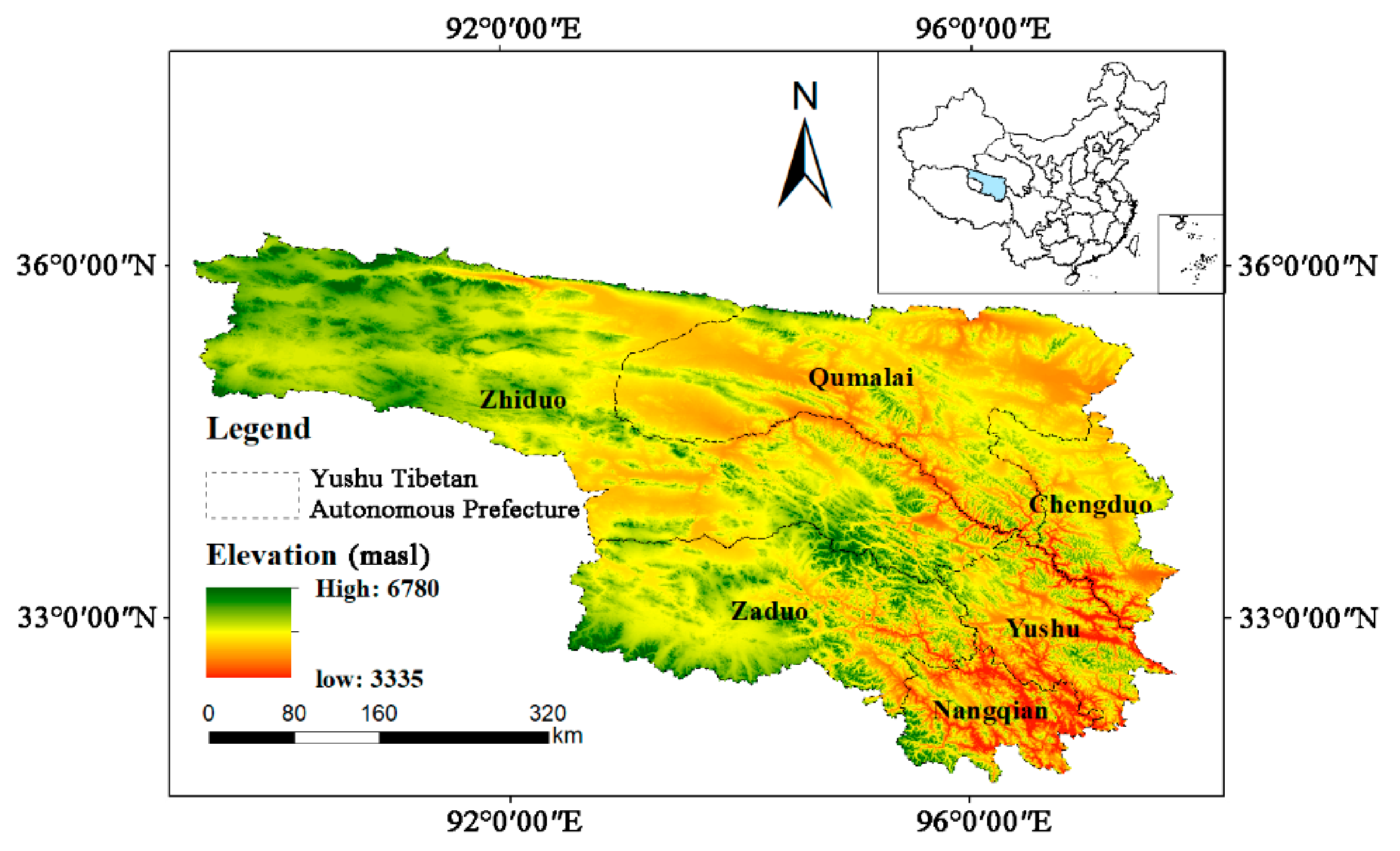
The study area (Figure 1), i.e., the Yushu Tibetan Autonomous Prefecture in the southwest of Qinghai Province, is located at the source of the Three Rivers in the hinterland of the Qinghai–Tibet Plateau (89°27′ to 97°39′ east (E), 31°45′ to 36°10′ north (N)). The Yushu Tibetan Autonomous Prefecture covers a total land area of 267,000 m2, which accounts for 37.2% of the Qinghai Province area. The area is surrounded by the Bayan Har Mountains, next to the Guoluo Tibetan Autonomous Prefecture in the east, the Ganzi Tibetan Autonomous Prefecture of Sichuan Province in the south, the Bayingeleng Mongolian Tibetan Autonomous Prefecture in the west, and the Haixi Mongolian and Tibetan Autonomous Prefecture in the north. With little noticeable interannual difference in the annual average temperature of 2 °C and precipitation of about 487 mm, the typical plateau paramo climate and special terrain conditions with a mean altitude above 4.2 km interact with each other and generate a distinctive natural environment with a unique vegetation distribution. The main water supply is from rainfall and snow melting. The Yushu Tibetan Autonomous Prefecture is the headstream of the Yangtze River, the Yellow River, and the Lancang River, where the San Jiangyuan nature reserve and the Hoh Xil nature reserve with the highest altitude cover the whole territory, highlighting its irreplaceable ecological status. Moreover, the Yushu Tibetan Autonomous Prefecture, including the six counties of Yushu, Zaduo, Chengduo, Zhiduo, Nangqian and Qvmalai, is inhabited by 14 ethnic groups (Han, Hui, Tu, Sala, Mongolia, etc.), accounting for 96.5% of the Tibetan population; accordingly, it holds enormous cultural value [39]. The religion of most of the population is Buddhism, which was introduced to the region about 1400 years ago. Over the past hundreds of years, many temples have been constructed as religious centers for ceremonies and activities. Temples are perceived as the Holy Lands of the Tibetans. By protecting these sacrosanct temples and their surrounding environment, Tibetans express their worship of religion. According to the previous field investigation results, we found that forests tended to concentrate around the temples and villages. Thus, we sought to research the influence of natural and cultural factors on the change in plateau forests through time.
2.2. Data Collection
Land-use data of 1990, 1995, 2000, 2005, 2010 and 2015 were used for this study. They were obtained from the Data Center for Resources and Environmental Sciences, Chinese Academy of Sciences (RESDC) (http://www.resdc.cn/ (accessed on 23 March 2021)), with a spatial resolution of 30 m. The spatial elevation data were obtained from the Geospatial data cloud (http://www.gscloud.cn/ (accessed on 23 March 2021)), with a spatial resolution of 30 m. The data were preprocessed using ArcGIS 10.4. In order to ensure the accuracy of data calculation, firstly, all data were registered, and then all raster data and vector data were subjected to raster projection and defined projection, respectively. The projection coordinates were Beijing_1954_3_Degree_GK_CM_108E.
The slope factor was divided into five slope gradients according to the Chinese slope standard classification [39], including 0–2°, 2–6°, 6–15°, 15–25°, 25–27°. The altitude factor was divided into five gradients according to previous research [40]: 3568–4333 meters above sea level (masl), 4333–4624 masl, 4624–4828 masl, 4828–5055 masl, and 5055–6300 masl. The forest landscape was classified into four categories: closed forest land, shrubbery, open forest land, and other forest land. Specifically, a canopy density greater than 30% and less than 40% was denoted as closed forest land, a canopy density greater than 40% was denoted as shrubbery, and a canopy density greater than 10% and less than 30% was denoted as open forest land. The remaining landscape was denoted as other forest land. Two vector point datasets were used, including 180 temples and 448 villages located in six counties. The temples and villages were stored as shape files with their locations and names by Arc GIS 10.4. Data regarding the village locations in the study area were obtained from the Qinghai geographic information center [41], and data regarding the temples were obtained from a field survey.
2.3. Methods
2.3.1. Spatial Sampling Analysis of Terrain Factors and Forest Landscape
In ArcMap 10.4, the elevation raster data of the Yushu Tibetan Autonomous Prefecture and the land use data are constructed as a unified grid quadrat, and superimposed to obtain the composite layer after sampling. Reclassification was used to extract 5 altitude gradient transects and 5 slope gradient transects. Using altitude and slope as a mask, four forest distributions at different altitudes and slopes were extracted. Then, we calculated the proportion of each forest landscape.
2.3.2. Correlation between Terrain Factors and Forest Landscape Distribution Patterns and Nonlinear Regression Tests
Since the relationship between terrain factors and forest landscape distribution is correlation rather than parallel, we use Statistical Product and Service Solutions (SPSS) for common correlation analysis. The geographical environment of the Yushu Tibetan Autonomous Prefecture in Qinghai Province is relatively complicated, especially the two topographic factors of altitude and slope, which have a certain impact on the distribution of forests [40]. We use 5 altitude gradients and 5 slope gradients to perform regression analysis on the area of the corresponding three forest types to explore the relationship between altitude, slope and forest area. Based on SPSS software, this paper uses regression models to explore the influence of altitude and slope on Yushu forests. Altitude and three forest landscapes accord with the quadratic Polynomial Function and Logarithmic Function in nonlinear regression analysis.
Through a mass of nonlinear curve fitting, the effect of slope factor on the distribution of four kinds of forest landscape accords with Peak Functions-Gauss Amp:
where A is amplitude; y0 is offset; xc is center; w is width.
There was no distribution of other forest land in 1990, and its proportion in the rest of the year was very small, which was of no research significance, so we did not perform regression analysis on other forest land.
2.3.3. Spatial Relationship Function of Temple, Village and Forest Landscapes
We use the Pc(rq) function to measure the spatial relationship between temples, villages and forest landscapes. The definition of Pc(rq) index is: the ratio of the density of a certain kind of land use change in the area of different radius r around the research point to the same kind of land use change density in the research area. This function can characterize the quantitative measurement of the spatial relationship between research points (temples and villages) and specific land use change areas over a series of radius distances. If the Pc(rq) value of a certain land use change is higher, it means that the corresponding culture represented by the research point has a greater impact on this land change, and the spatial relationship is more concentrated. In order to correct the problem that multiple research areas may overlap, which may lead to repeated calculations of land use, Thiessen polygons will be generated around the research points to divide the entire research area into non-overlapping spaces [38]. Then, for all points in the study area, their spatial area at a certain radius distance r will be clipped by their Thiessen polygon; thus, only land use changes that belong to both the radius r and the Thiessen polygon are included in the calculation range. In a given series of radius distances rq, the Pc(rq) spatial relationship function of a specific land use change can be expressed as:
In the formula, n is the total number of research points (monasteries, villages) in the research area; m is the number of polygons (the area where land use changes have occurred); Pi(rq) represents the different research radii generated around the research point i. The circular area of rq (r1 = 1 km, r2 = 2 km..., r10 = 10 km). Rcj represents the polygon j of the land use change type c; ρc is the density of the specific type of land use change c in the research area; Ti represents the Thiessen polygon generated from the research point i; TA is the research area. In addition, the symbol ∩ refers to the intersection of different spatial regions; the function Area { } calculates the area of all spatial ranges within the brackets. In the formula, Scxy represents the area of land use type transferred from x to y within a certain spatial range, c represents all the types of transfers related to land-use type c that occurred during the research period, x represents the type before the land-use type transfer occurs, and y represents the type of land transfer.
2.3.4. Monte Carlo Significance Test of Pc(rq) Function
The Pc(rq) function can reflect the spatial relationship between the research point and the surrounding land use changes, but in order to make the result of this function more credible, this article will use the Monte Carlo random test model to test the significance. First, the Monte Carlo test will generate a set of point data sets containing n random points in the study area, where n is determined by the actual number of study points (monasteries, villages). Then, it will generate a set of circular neighborhoods with different radii rq (r1 = 1 km, r2 = 2 km..., r10 = 10 km) centered on the research point and their Thiessen polygons, so as to determine the circular neighborhoods and Thiessen polygons at the same time as m land use change polygons. For the Pc(rq) function, m polygons are specific types of land use change. Repeat the calculation of the Pc(rq) function 999 times, and sort the 999 expected values together with the observed index values according to their size. Finally, the 5th percentile and 95th percentile of the 999 indicators were set as the lower limit of the confidence interval and the upper limit of the confidence interval, respectively. If the observed value is greater than the upper limit of the confidence interval determined according to the expected value, it means that the spatial relationship between the research site and surrounding land use changes is significant, and the land use changes are significantly clustered relative to the research site. If the observed value is less than the lower limit of the confidence interval, it indicates that the spatial relationship between the research site and surrounding land use changes is also significant, but the land use change is significantly separated from the research site. If the value of the indicator is between the upper limit and the lower limit, it indicates that there is no definite spatial relationship between the research site and the land use change. If the land use change occurs randomly around the research site, at the same time, it shows that temples and villages are not important factors driving land use changes.
2.3.5. The Establishment of Buffer Zone
In order to further explore the influence of temples on the distribution of the three forest landscapes, we set up a buffer zone with the temple as the center and r as the radius (r1 = 1 km, r2 = 2 km..., r10 = 10 km), and calculated the proportions of the three forest landscapes in the buffer zone in the 6 periods of land use data from 1990 to 2015.
3. Results
3.1. Spatiotemporal Variation Characteristic of Forest Landscape as a Function of Altitude and Slope
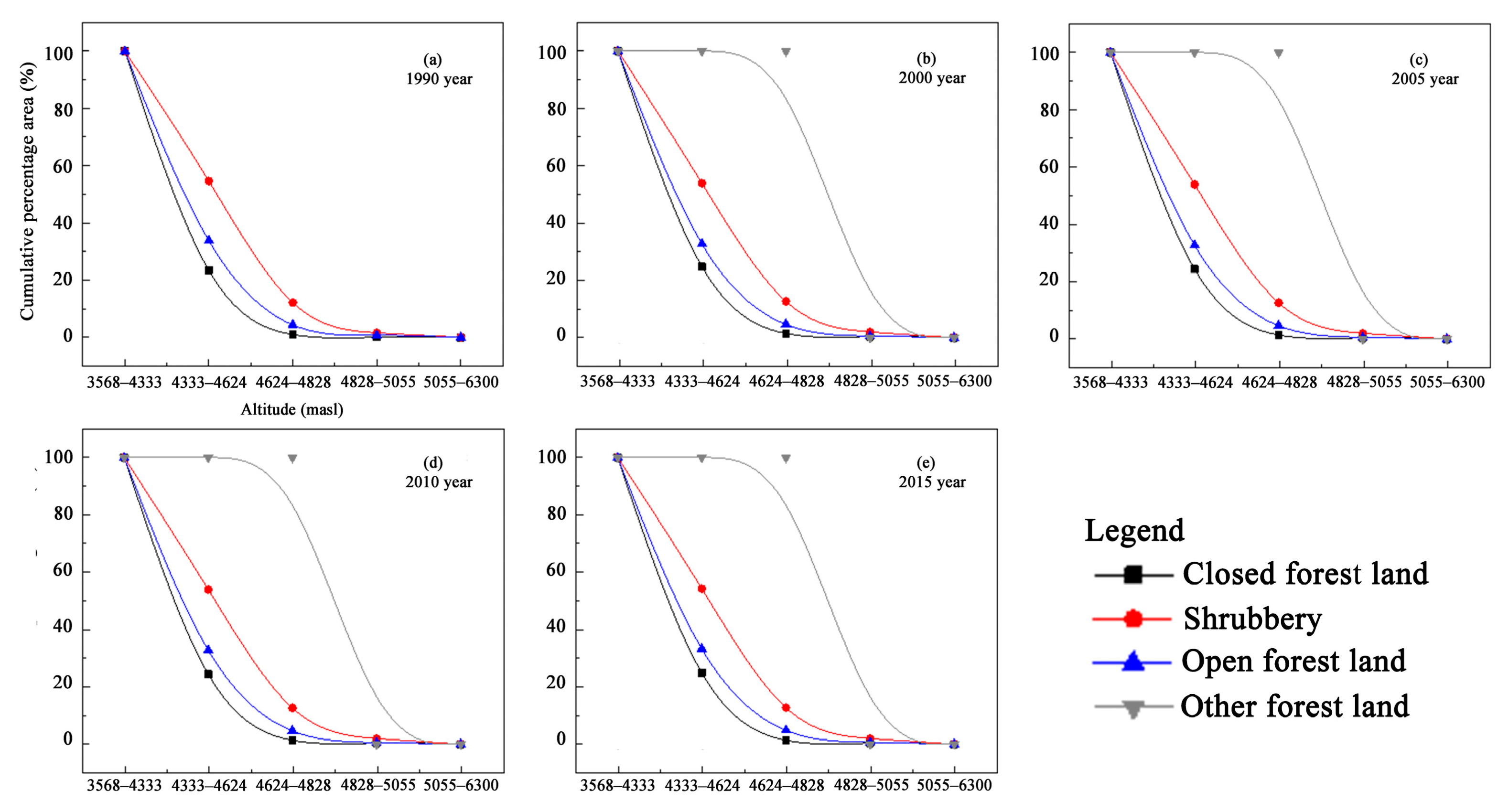
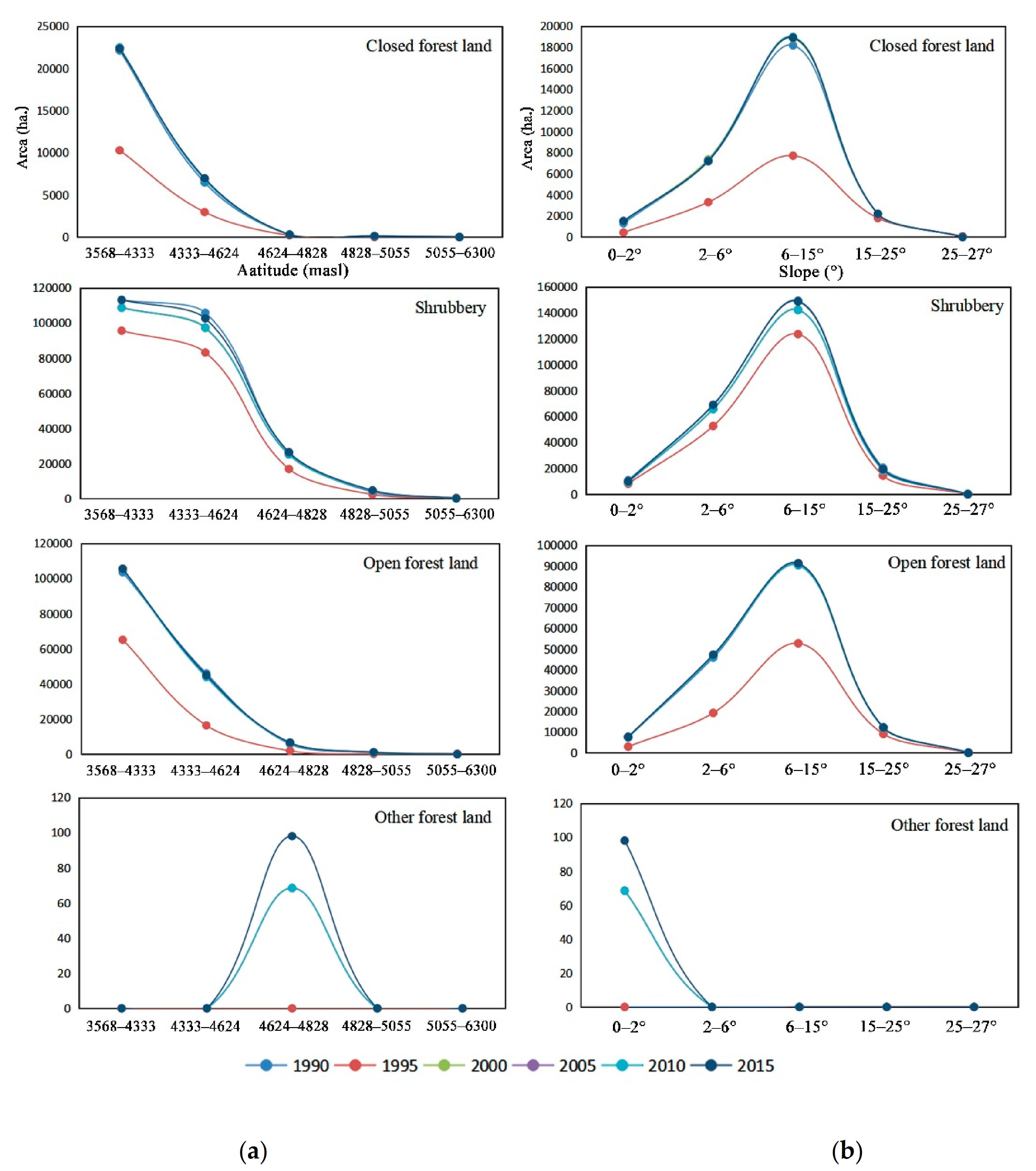
From the perspective of the influence of altitude on the spatial distribution of the forest landscape (Figure 2), the distribution range of the four forest landscapes was between 3568 masl and 6300 masl. Among them, shrubbery covered the widest range, widely distributed throughout Qinghai Province. Closed forest land was mainly distributed in the relatively low altitude range (3568–4333 masl), and there was no closed forest land above 5055 masl. The smallest category of other forest land was only distributed in the altitude range of 3568–4828 masl. The four forest landscapes had the same distribution law, whereby the distribution area increased as the altitude increased. Specifically, the areas of closed forest land, shrubbery, and open forest land decreased sharply in the altitude range of 3568–4624 masl, while other forest land decreased sharply in the range of 4624–5055 masl.
From the perspective of the influence of slope on the spatial distribution of forests, the four forest landscapes were distributed in the range of 0–27°. Specifically, the areas with slopes greater than 25° had no closed forest land distribution, and other forest land was only distributed in the 0–2° range. According to the distribution law, as the slope increased, the distribution of the four forest landscapes showed a trend of first rising and then decreasing sharply.
In addition, Figure 3 shows that, among the four forest landscapes, the area of shrubbery was the largest regardless of the elevation gradient or the slope gradient, followed by open forest land and closed forest land, whereas the smallest area constituted other forest land. This finding is related to the fact that shrub is generally more adaptable to harsh environments than arbor. In terms of time, from 1990 to 2015, the areas of closed forest land, shrubbery and open forest land manifested fluctuations within a narrow range.
3.2. Regression Model Analysis of Terrain Factors
In our research, the aim was to evaluate the relationship between forest distribution and terrain factors including altitude and slope. Statistical analysis methods have shown a correlation rather than a parallel relationship between forest distribution and topographic factors; thus, we applied regression analysis using SPSS instead of common correlation analysis [41]. The laws of forest distribution under the influence of altitude and slope were similar in that they were both nonlinear. On the other hand, they each fit different functions according to the fitting results (Table 1 and Table 2).
As other forest land featured too few samples at some altitudes and slope gradients, we omitted it from the analysis. For closed forest land and open forest land, the effect of altitude on the distribution of the forest landscape conformed to the polynomial function/quadratic polynomial in nonlinear regression analysis. Fisher’s test [35] was applied, whereby a mean R2 > 0.95, p < 0.05, and F > 19.00 indicated a significant relationship between altitude and the distributions of closed forest land and open forest land.
Compared with the aforementioned two types of forest, the relationship between altitude and shrubbery showed a better fit with a logarithmic function in linearizable non-linear regression analysis. Here, Fisher’s test with a mean R2 > 0.83, p < 0.05, and F > 10.13 indicated a significant negative relationship between altitude and the distribution of shrubbery.
According to nonlinear curve fitting, the effect of slope on the distribution of the three kinds of forest landscape followed the amplitude version of a Gaussian peak function. Here, a mean R2 > 0.99 and p < 0.05 indicated a significant relationship between slope and the distribution of the four types of forest landscape. During the five periods, the slope element had the same effect on the three types of forest distribution existing on an optimum slope, thus identifying it as an important factor affecting the forest landscape pattern.
3.3. Spatiotemporal Variation Characteristics of Forest Landscape as a Function of Different Cultural Landscapes
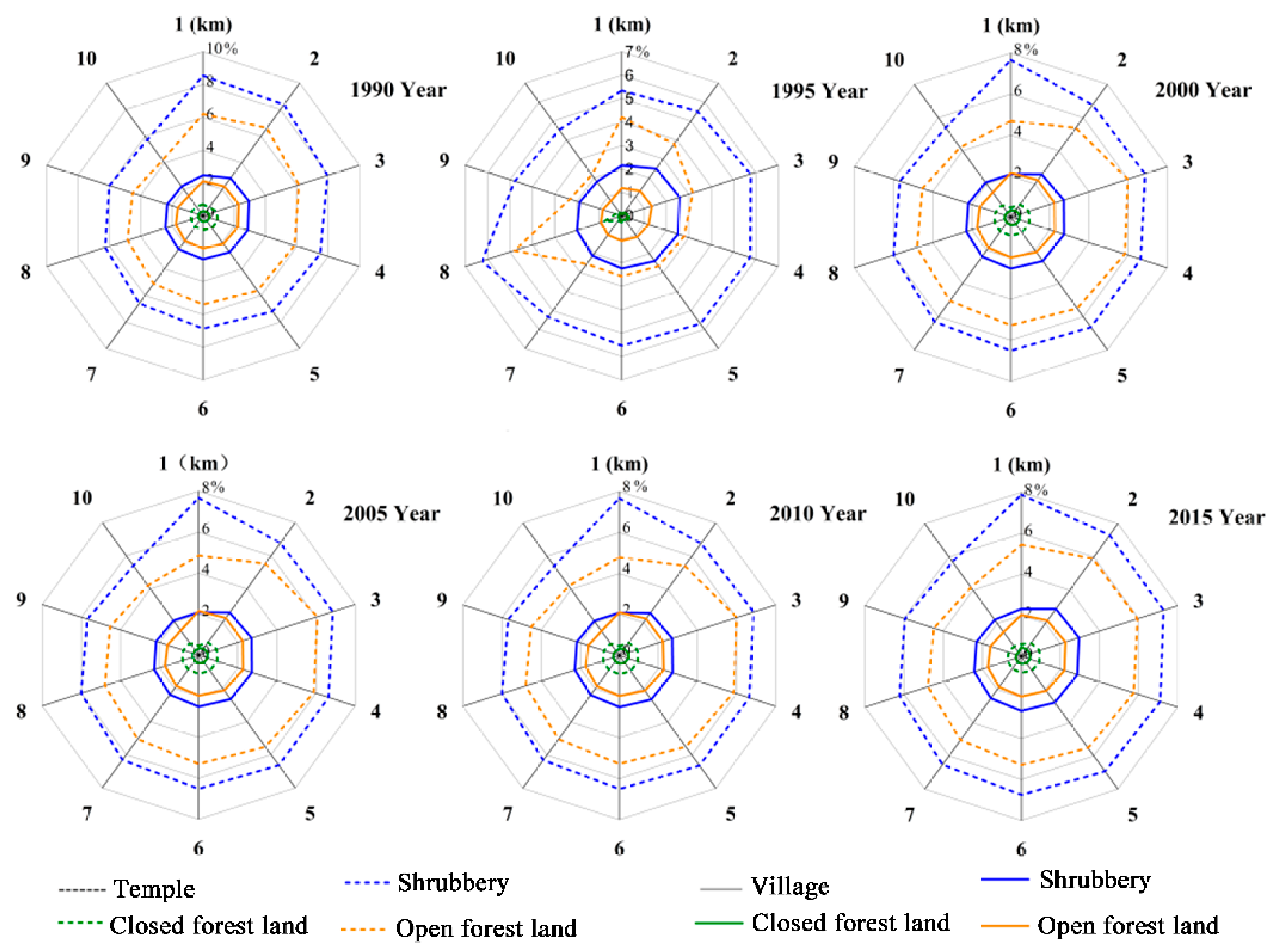
Figure 4 shows the percentage of closed forest land, shrubbery, and open forest land around the temples and villages within the different radii from 1990 to 2015, reflecting the influence of temples and villages on changes in the surrounding forest. The most distributed type of landscape around both temples and villages was shrubbery, followed by open forest land and lastly closed forest land. This indicates that forest distribution was potentially affected by the cultural landscape. Table 3 shows the Pc(rq) values of conversion from grassland to forestland within a range of 1–10 km around temples and settlements. If the Pc(rq) value of a certain land use change is higher, it means that the corresponding culture represented by the research point has greater impact on this land change. The results showed that the Pc(rq) value around temples was higher, and it continued to increase from 1990 to 2015.
As the distance increased from 1 km to 10 km, the area of every type of forest around the temples (represented by a dashed line) generally increased with respect to that around the villages across all study periods. This result proves that temples play a more crucial role in influencing forest distribution compared to villages. In addition, there was an obvious contrast in the percentage of forest around temples and villages within 6 km being larger than that beyond 6 km. This indicates that beyond 6 km, the influence of temples was weakened.
3.4. Spatiotemporal Variation Characteristic of Forest Landscape under the Influence of Temples
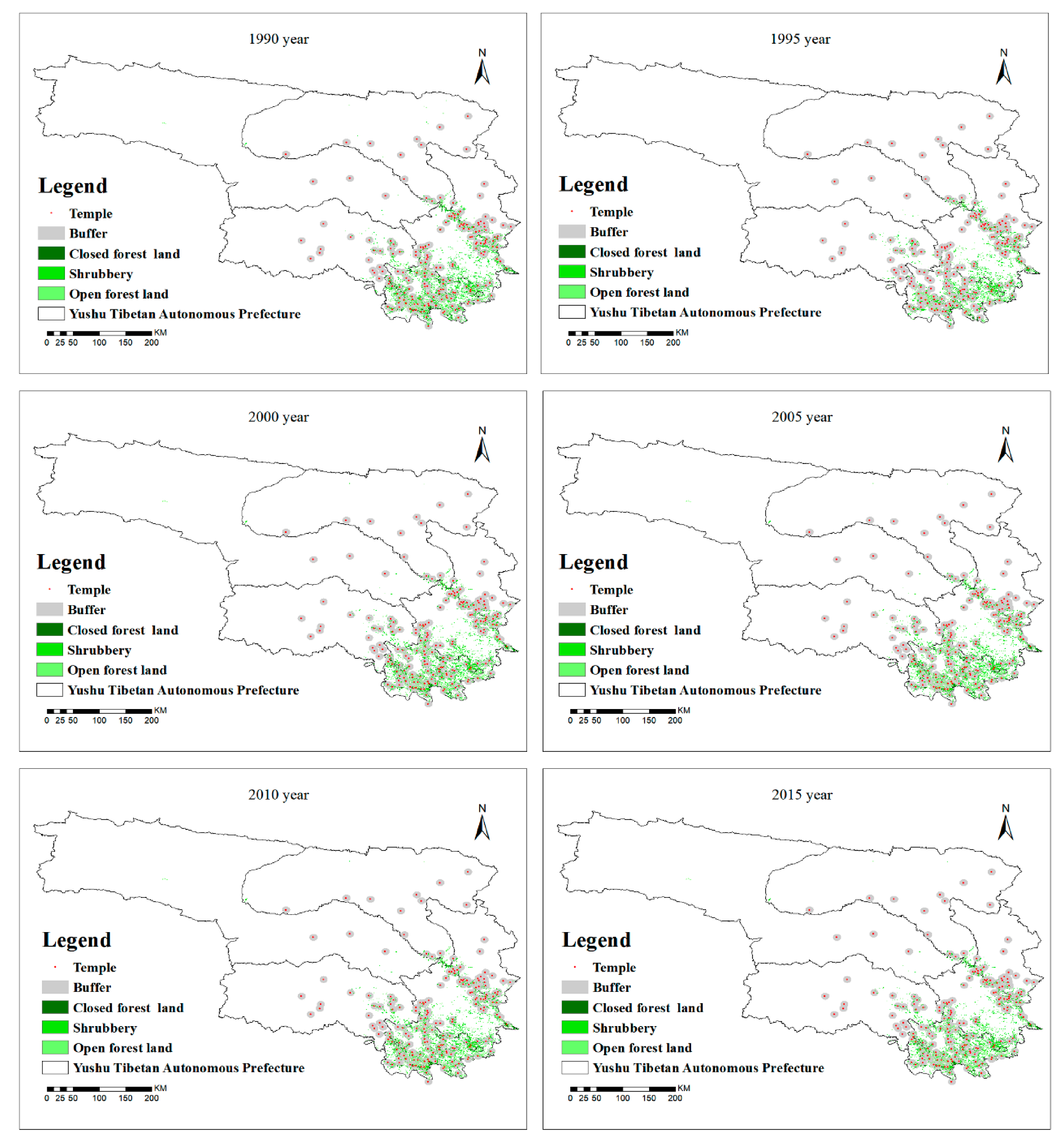
The previous result showed a significant influence of temples on the forest landscape within 6 km. Therefore, we generated a buffer zone with a radius of 6 km (Figure 5) and calculated the percentage of forest area in the buffer zone with respect to the total forest area (Table 4).
Table 4 shows the distribution of the three forest landscapes within the significant range of temple influence from 1990 to 2015, reflecting the changes in the proportion of forest area in the Yushu Tibetan Autonomous Prefecture across different periods. Overall, the forest area distributed within 6 km around the temple from 1990 to 2015 accounted for 48.93%, 45.67%, 48.38%, 48.43%, 48.37%, and 48.38% of the total forest area, highlighting that half of the forest area of the Yushu Tibetan Autonomous Prefecture was distributed around the temple. Figure 5 also shows that more forest was distributed in areas with temples, indicating their positive effect. From the perspective of the distribution of the three different forest landscapes, from 1990 to 2015, shrubbery dominated, accounting for 25.42%, 30.13%, 24.68%, 24.70%, 24.70%, and 24.71% of the total forest area around the temple, respectively. This was followed by open forest land, which accounted for 20.08%, 13.80%, 20.17%, 20.22%, 20.17%, and 20.15% of the total forest area around the temple, respectively. Closed forest land had the lowest distribution, accounting for only 3.53% of the total forest area in the year with the highest proportion.
In terms of time, the proportion of the three forest landscapes around the temple fluctuated greatly from 1990 to 2000 and stabilized from 2000 to 2015. From 1990 to 2015, the shrubbery, open forest land, and closed forest land around the temple only changed by 0.09%, 0.71%, and 0.08%, respectively, and the total area of the three forest landscapes only changed by 0.54%. In general, although the forest landscape around the temple has increased or decreased across the 25 years, the overall change is small, indicating that the temples had a protective effect on the forest.
4. Discussion
4.1. The Influence of Terrain Factors on Forest Landscape Distribution
Terrain factors play an important role in the distribution of forest landscapes. The natural distribution of forests is usually affected by factors such as temperature, precipitation, altitude, soil, and sunshine. These influencing factors are closely related to the topographical conditions of an area. China has a vast territory spanning a wide range of latitudes, and its topography is relatively undulating, thus forming a diverse climate. Although the distribution of forests is greatly affected by climate, from the perspective of a large area, in terms of altitude distribution, research by Yang et al. [42] showed that the general trend of forest distribution in China is to decrease with the increase in altitude. However, in a study of forest distribution on the Qinghai–Tibet Plateau by Wang et al. [43], different results were recorded. Their research showed that when the altitude was lower than 3500 masl, the forest distribution increased with altitude, whereas when the altitude was higher than 3500 masl, the forest distribution showed the opposite trend. The study area of our research was the Yushu Tibetan Autonomous Prefecture, which is located on the Qinghai–Tibet Plateau, where the lowest altitude recorded was 3335 masl. The distribution of forests in our study was consistent with the results above. In high-altitude areas, the water and heat conditions gradually decline, becoming unfavorable for the growth of most vegetation. Therefore, at a certain altitude, there is a lesser natural distribution of forests. The most dominant forest type in the Yushu Tibetan Autonomous Region was shrubbery. This was due to the higher altitude of the plateau in cold areas, where it is easier for shrubbery to grow than trees.
The slope mainly affects the soil conditions, which in turn affect the distribution of the forest. First, a greater slope leads to less average rainfall per unit area and, thus, a greater loss of natural precipitation. Therefore, if the slope is too large, the water retention function of the soil is affected. Secondly, with erosion following natural rainfall, soil is lost in areas with large slopes, resulting in thin soil layers that are not suitable for forest growth. Lastly, the loss of water in the soil often leads to the removal of organic nutrients and inorganic salts, resulting in a decline in soil fertility, making it unsuitable for forest development. The relationship between slope and forest distribution closely followed a peak function, showing a correlation. However, from the perspective of natural conditions, this finding could not explain why the forest distribution reached its maximum value at 6–15°, rather than at 0–6°. We speculate that this is because the forested areas in the Yushu Tibetan Autonomous Prefecture are not completely natural ecosystems, but composite ecosystems disturbed by human activities. In flat plateau areas, human activities such as building villages, planting pastures, and grazing livestock hinder the expansion of forests.
4.2. The Influence of Culture Landscapes on Forest Distribution
Terrain factors affect the natural distribution of the forest, but human activities are becoming more frequent and their impact cannot be ignored. From a spatial point of view, the influence of temples in terms of human factors is significantly greater than that of villages. Many studies on human activities have shown that urban construction has an important impact on the surrounding land use, which is different from the results of this article. However, these studies usually ignore the influence of religious culture. In a previous study by Zhuoma et al., it was found that the proportion of degraded settlements in a 4 km buffer zone was higher than that of temples in the current study related to the distribution characteristics of temples and settlements and land use changes in the Yushu Tibetan Autonomous Prefecture [44]. Considering the results of the positive influence of temples on forest protection in this article, we speculate that this may be related to the traditional culture of the study area. The main ethnic group in the Yushu Tibetan Autonomous Prefecture constitutes the Tibetans, accounting for 95.6% of the Tibetan population. Tibetans have a strong religious culture, which may lead to greater impact on the distribution of forests. The results of the buffer zone showed that half of the forest is distributed within a 6 km range of the temples, highlighting their important role in forest distribution. This indicates the effects of religious culture within the Yushu Tibetan Autonomous Prefecture, as a function of the unique cultural concepts of Tibetans, who believe that nature is to be protected and life is to be cherished [45]. They believe that humans should respect nature, obey the laws of natural existence, and worship nature with sacred mountains and waters. Accordingly, the Tibetan worship of natural gods plays a vital role in protecting the forest resources of the sacred mountain. Furthermore, Tibetan temples are mostly built on the side or foot of the mountain. For example, the famous Jiegu Temple is located on the Meima Mountain in Beimuta. Therefore, forest landscapes affected by religious culture are protected to a certain extent, and there is a greater degree of protection in areas where temples are present. This is of great significance for land management and planning in ethnic cultural areas.
The proportion of the forest landscape around the temples only decreased by 0.54% from 1990 to 2015, and the change was small. However, there were fluctuations from 1990 to 2000, which may be related to the policies implemented by Qinghai Province. The Yushu Tibetan Autonomous Prefecture is an area where animal husbandry is the main source of income. Compared with forests, grassland has higher economic value. In 1990, Qinghai Province issued the “Decision on Accelerating the Development of Animal Husbandry” to vigorously develop an economic policy focusing on animal husbandry. Therefore, from 1990 to 1995, the forest area was reduced to develop animal husbandry. In 1996, Qinghai Province passed the “Measures of the Qinghai Province forImplementing the Forest Law of the People’s Republic of China” with the aim of protecting rationally developing and utilizing forest resources and maintaining ecological balance. Thus, people experienced renewed awareness of the importance of ecological protection, thereby restoring the forests around the temples affected by human activities. In general, in the process of economic development, the area of forest land can be maintained, and the protection of religious culture is an important factor.
Since most of the studies on temples located on the Qinghai–Tibet Plateau were within the field of social sciences, there were very few studies related to land use with which we could compare our results. As the theory and methods describing the influence of religious culture on the ecological environment are not perfect, this article attempted to use the Pc(rq) function and the establishment of a buffer zone for quantitative analysis, but the results still need further verification.
5. Conclusions
Terrain factors affect the natural distribution of forests, and human factors affect the scale of forest distribution. The distribution area of the four forest landscapes decreased with the increase in altitude, whereas with the increase in slope, the area first gradually increased and then decreased sharply. The most dominant forest type was shrubbery. According to the regression analysis and hypothetical tests, both slope and altitude had a significant correlation with the distribution pattern of the four types of forest landscape. The influence of altitude on closed forest land and open forest land followed a polynomial function, while that on shrubbery followed a logarithmic function, and the impact of slope on the three forest landscapes followed the amplitude version of a Gaussian peak function. In terms of cultural factors, temples had a greater impact on the forest than villages, leading to a higher forest density in their proximity as a function of their protection under religious culture. However, beyond 6 km, this influence weakened. Over 25 years, the proportion of forest area did not change significantly.
Author Contributions
Conceptualization, N.C. and L.G.; methodology, N.C. and H.Z.; software and formal analysis, M.Z.; investigation, L.G.; resources, N.C. and H.Z.; data curation, N.C. and H.Z.; writing—review and editing, L.G.; project administration, L.G.; funding acquisition, L.G. All authors have read and agreed to the published version of the manuscript.
Funding
This research was funded by the Second Tibetan Plateau Scientific Expedition and Research (STEP) program (2019QZKK0308) and the Ministry of Science and Technology of China (2017YFC0505601).
Acknowledgments
We are grateful for the comments of the anonymous reviewers, which greatly improved the quality of this paper.
Conflicts of Interest
The authors declare no conflict of interest.
References
- Balmford, A.; Moore, J.L.; Brooks, T.; Burgess, N.; Hansen, L.A.; Williams, P.; Rahbek, C. Conservation Conflicts Across Africa. Science 2001, 291, 2616–2619. [Google Scholar] [CrossRef]
- Pimm, S.L.; Raven, P. Extinction by numbers. Nature 2000, 403, 843–845. [Google Scholar] [CrossRef]
- Sala, O.E.; Chapin, F.S.; Armesto, J.J.; Berlow, E.L.; Bloomfield, J.B.; Dirzo, R.H.; Huber-Sanwald, E.; Huenneke, L.F.; Jackson, R.B.; Kinzig, A.P.; et al. Global biodiversity scenarios for the Year 2100. Science 2000, 287, 1770–1774. [Google Scholar] [CrossRef]
- Teixeira, A.M.G.; Soares-Filho, B.S.; Freitas, S.R.; Metzger, J.P. Modeling landscape dynamics in an Atlantic Rainforest region: Implications for conservation. For. Ecol. Manag. 2009, 257, 1219–1230. [Google Scholar] [CrossRef]
- Ayram, C.A.C.; Mendoza, M.E.; Etter, A.; Salicrup, D.R.P. Potential Distribution of Mountain Cloud Forest in Michoacán, Mexico: Prioritization for Conservation in the Context of Landscape Connectivity. Environ. Manag. 2017, 60, 86–103. [Google Scholar] [CrossRef]
- Spracklen, D.V.; Righelato, R. Tropical montane forests are a larger than expected global carbon store. Biogeosci. Discuss 2013, 10, 18893–18924. [Google Scholar] [CrossRef] [Green Version]
- Feng, X.; Wu, X.; Shen, D.; Zhu, J. Association analysis of forest topography and vegetation spatial pattern based on DEM. Fujian For. Sci. Technol. 2015, 1, 26–30. [Google Scholar] [CrossRef]
- Zeng, H.D. Application of Digital Terrain Information and Geostatistics to Forest Spatial Pattern Analysis—A Case on Wuyi Mt. Area. Geoinf. Sci. 2005, 2, 82–88. [Google Scholar] [CrossRef] [Green Version]
- Andrews, A. Fragmentation of Habitat by Roads and Utility Corridors: A Review. Aust. Zool. 1990, 26, 130–141. [Google Scholar] [CrossRef] [Green Version]
- Collinge, S.K. Ecological consequences of habitat fragmentation: Implications for landscape architecture and planning. Landsc. Urban Plan. 1996, 36, 59–77. [Google Scholar] [CrossRef]
- Linehan, J.; Gross, M.; Finn, J. Greenway planning: Developing a landscape ecological network approach. Landsc. Urban Plan. 1995, 33, 179–193. [Google Scholar] [CrossRef]
- Walker, R.; Craighead, L. Analyzing Wildlife Movement Corridors in Montana Using GIS. In Proceedings of the 1997 ESRI User Conference, Redlands, CA, USA, 8–11 July 1997. [Google Scholar]
- Deng, X.; Huang, J.; Rozelle, S.; Uchida, E. Growth, population and industrialization, and urban land expansion of China. J. Urban Econ. 2008, 63, 96–115. [Google Scholar] [CrossRef]
- Castella, J.C.; Kam, S.P.; Dang, D.Q.; Verburg, P.H.; Chu, T.H. Combining top-down and bottom-up modelling approaches of land use/cover change to support public policies: Application to sustainable management of natural resources in northern Vietnam. Land Use Policy 2007, 24, 531–545. [Google Scholar] [CrossRef]
- Rosati, L.; Fipaldini, M.; Marignani, M.; Blasi, C. Effects of fragmentation on vascular plant diversity in a Mediterranean forest archipelago. Bot. Ital. 2010, 144, 38–46. [Google Scholar] [CrossRef]
- Bürgi, M. A case study of forest change in the Swiss lowlands. Landsc. Ecol. 1999, 14, 567–576. [Google Scholar] [CrossRef]
- Xin, C.; Chen, J.; Chen, L.J.; Liao, A.P.; Sun, F.D.; Yang, L.I.; Lei, L.I. Preliminary analysis of spatiotemporal pattern of global land surface water. Sci. China Earth Sci. 2014, 57, 2330–2339. [Google Scholar] [CrossRef]
- Kazak, J.; Wang, T.; Szewrański, S. Analysis of Land Use Transformation Potential in Spatial Management. Real Estate Manag. Valuat. 2015, 23, 5–14. [Google Scholar] [CrossRef] [Green Version]
- Zhang, Z.; Zinda, J.A.; Li, W. Forest transitions in Chinese villages: Explaining community-level variation under the returning forest to farmland program. Land Use Policy 2017, 64, 245–257. [Google Scholar] [CrossRef] [Green Version]
- Jamon, V.D.H.; Ozdogan, M.; Burnicki, A.; Zhu, A.X. Evaluating forest policy implementation effectiveness with a cross-scale remote sensing analysis in a priority conservation area of Southwest China. Appl. Geogr. 2014, 47, 177–189. [Google Scholar] [CrossRef]
- Cullotta, S.; Barbera, G. Mapping traditional cultural landscapes in the Mediterranean area using a combined multidisciplinary approach: Method and application to Mount Etna (Sicily; Italy). Landsc. Urban Plan. 2011, 100, 98–108. [Google Scholar] [CrossRef]
- Jiao, Y.; Liang, L.; Okuro, T.; Takeuchi, K. Ecosystem Services and Biodiversity of Traditional Agricultural Landscapes: A Case Study of the Hani Terraces in Southwest China. In Biocultural Landscapes; Springer: Dordrecht, The Netherlands, 2014; pp. 81–88. [Google Scholar] [CrossRef]
- Grace, D.; Jeuland, M. Preferences for Attributes of Sacred Groves and Temples along an Urbanization Gradient in the National Capital Region of India. Ecol. Econ. 2018, 152, 322–335. [Google Scholar] [CrossRef]
- Bhagwat, S.A.; Nogué, S.; Willis, K.J. Cultural drivers of reforestation in tropical forest groves of the Western Ghats of India. For. Ecol. Manag. 2014, 329, 393–400. [Google Scholar] [CrossRef] [Green Version]
- Chen, J.; Yifang, B.; Songnian, L. China: Open access to Earth land-cover map. Nature 2014, 514, 434. [Google Scholar] [CrossRef] [Green Version]
- Kuenzer, C.; Leinenkugel, P.; Vollmuth, M.; Dech, S. Comparing global land-cover products—Implications for geoscience applications: An investigation for the trans-boundary Mekong Basin. Int. J. Remote Sens. 2014, 35, 2752–2779. [Google Scholar] [CrossRef] [Green Version]
- Leinenkugel, P.; Kuenzer, C.; Oppelt, N.; Dech, S. Characterisation of land surface phenology and land cover based on moderate resolution satellite data in cloud prone areas—A novel product for the Mekong Basin. Remote Sens. Environ. 2013, 136, 180–198. [Google Scholar] [CrossRef]
- Chen, J.; Chen, J.; Liao, A.; Cao, X.; Chen, L.; Chen, X.; He, C.; Han, G.; Peng, S.; Lu, M. Global land cover mapping at 30 m resolution: A POK-based operational approach. ISPRS J. Photogramm. Remote Sens. 2015, 103, 7–27. [Google Scholar] [CrossRef] [Green Version]
- Vemu, S.; Bhaskar, P.U. Change Detection in Landuse and landcover using Remote Sensing and GIS Techniques. Int. J. Eng. Sci. Technol. 2010, 2, 7758–7762. [Google Scholar]
- Balogun, I.A.; Adeyewa, D.Z.; Balogun, A.A.; Morakinyo, T.E. Analysis of urban expansion and land use changes in Akure, Nigeria, using remote sensing and geographic information system (GIS) techniques. J. Geogr. Reg. Plan. 2011, 4, 533–541. [Google Scholar]
- Hu, Z.; Lo, C.P. Modeling urban growth in Atlanta using logistic regression. Comput. Environ. Urban Syst. 2007, 31, 667–688. [Google Scholar] [CrossRef]
- Qi, W.; Meng, J.; Mao, X. Scenario simulation and landscape pattern assessment of land use change based on neighborhood analysis and auto-logistic model: A case study of Lijiang River Basin. Geogr. Res. 2014, 33, 1073–1084. [Google Scholar]
- Basse, R.M.; Omrani, H.; Charif, O.; Gerber, P.; Bódis, K. Land use changes modelling using advanced methods: Cellular automata and artificial neural networks. The spatial and explicit representation of land cover dynamics at the cross-border region scale. Appl. Geogr. 2014, 53, 160–171. [Google Scholar] [CrossRef]
- Bryan, C.P.; Daniel, G.B.; Gaurav, A.M. Using neural networks and GIS to forecast land use changes: A Land Transformation Model. Comput. Environ. Urban Syst. 2002, 26, 553–575. [Google Scholar] [CrossRef]
- Kamusoko, C.; Aniya, M.; Adi, B.; Manjoro, M. Rural sustainability under threat in Zimbabwe—Simulation of future land use/cover changes in the Bindura district based on the Markov-cellular automata model. Appl. Geogr. 2009, 29, 435–447. [Google Scholar] [CrossRef]
- Poelmans, L.; Rompaey, A.V. Complexity and performance of urban expansion models. Comput. Environ. Urban Syst. 2010, 34, 17–27. [Google Scholar] [CrossRef]
- Verburg, P.H.; Soepboer, W.; Veldkamp, A. Modeling the Spatial Dynamics of Regional Land Use: The CLUE-S Model. Environ. Manag. 2002, 30, 391. [Google Scholar] [CrossRef]
- Ran, Y.H.; Xin, L.I.; Institute, E.E.; Sciences, C.A.O. First comprehensive fine-resolution global land cover map in the world from China—Comments on global land cover map at 30-m resolution. Sci. China 2015, 58, 1677–1678. [Google Scholar] [CrossRef]
- Ministry of Land and Resources of the People’s Republic of China. TD/T 1055-2019, Technical Regulation of the Third Nationwide Land Survey. Available online: http://gi.mnr.gov.cn/201901/t20190129_2391915.html (accessed on 2 June 2019).
- Cui, N.; Luo, G.; Du, S. Analysis of Spatial-Temporal Variation of Grassland Landscape Pattern Based on Terrain Factors in Qinghai Yushu Tibetan Autonomous Prefecture, China. In Proceedings of the 26th International Conference on Geoinformatics, Kunming, China, 28–30 June 2018. [Google Scholar]
- Qinghai Information Center. Available online: http://www.qhei.org.cn/ (accessed on 11 May 2019).
- Yang, Y.; Zhang, X.; Yu, H.; Lv, Z. The Spatial Distribution of China’s Forest Biomass and Its Influencing Factors. J. Southwest For. Univ. 2015, 35, 45–52. [Google Scholar] [CrossRef]
- Wang, X.; Ke, B.; Huang, Z.; Yang, G.; Huang, G.; Hu, Q.; Sun, L. Quantification of Forest Carbon Storage in Tibetan Plateau. For. Environ. Sci. 2020, 36, 9–19. [Google Scholar]
- Zhuo-Ma, C.; Huang, Q.; Guo, L.; Xue, D.Y. Distribution and Dynamic Change of Land Use of Monastery and Settlement in YuShu Tibetan Autonomous Prefecture in Three River Headwater Region. J. Minzu Univ. China 2016, 25, 5–11. [Google Scholar]
- Wei, F.U.; Junquan, Z.; Guozhen, D.U. Research on tibetan traditional ecological ethics and the qinghai- tibet plateau ecological and environmental protection. Ecol. Econ. 2013, 2, 420–423. [Google Scholar]
Figure 1.
Location of study area.

Figure 2.
Cumulative distribution curves of four types of forest landscape for 5 periods.

Figure 3.
(a) Area distribution of forest landscape in different altitude ranges. (b) Area distribution of forest landscape in different slope ranges.
Figure 3.
(a) Area distribution of forest landscape in different altitude ranges. (b) Area distribution of forest landscape in different slope ranges.

Figure 4.
The percentage of three types of forest around the temples and villages from 1990 to 2015.
Figure 4.
The percentage of three types of forest around the temples and villages from 1990 to 2015.

Figure 5.
The distribution of temples and forest landscape from 1990 to 2015.


Table 1.
Regression analysis on altitude element and distribution of three types of forest landscape.
Table 1.
Regression analysis on altitude element and distribution of three types of forest landscape.
| Year | R2 | F | p | ||||||
|---|---|---|---|---|---|---|---|---|---|
| Closed Forest Land | Shrubbery | Open Forest Land | Closed Forest Land | Shrubbery | Open Forest Land | Closed Forest Land | Shrubbery | Open Forest Land | |
| 1990 | 0.977 | 0.863 | 0.993 | 41.647 | 18.843 | 141.443 | 0.023 | 0.023 | 0.007 |
| 2000 | 0.979 | 0.884 | 0.993 | 46.457 | 22.907 | 145.416 | 0.021 | 0.017 | 0.007 |
| 2005 | 0.978 | 0.883 | 0.993 | 43.882 | 22.640 | 145.372 | 0.022 | 0.018 | 0.007 |
| 2010 | 0.978 | 0.878 | 0.993 | 43.882 | 21.571 | 146.769 | 0.022 | 0.019 | 0.007 |
| 2015 | 0.979 | 0.878 | 0.993 | 47.119 | 21.571 | 152.407 | 0.021 | 0.019 | 0.007 |
Table 2.
Regression analysis on slope element and distribution of three types of forest landscape.
| Year | R2 | p | ||||
|---|---|---|---|---|---|---|
| Closed Forest Land | Shrubbery | Open Forest Land | Closed Forest Land | Shrubbery | Open Forest Land | |
| 1990 | 0.987 | 0.988 | 0.986 | 0.012 | 0.010 | 0.011 |
| 2000 | 0.984 | 0.991 | 0.985 | 0.014 | 0.009 | 0.012 |
| 2005 | 0.984 | 0.991 | 0.985 | 0.014 | 0.009 | 0.012 |
| 2010 | 0.984 | 0.991 | 0.986 | 0.014 | 0.009 | 0.011 |
| 2015 | 0.982 | 0.990 | 0.985 | 0.015 | 0.010 | 0.011 |
Table 3.
The Pc(rq) value of conversion from grassland to forestland in 1–10 km buffer.
| Point | Year | Pc(rq) | |||||||||
|---|---|---|---|---|---|---|---|---|---|---|---|
| 1 km | 2 km | 3 km | 4 km | 5 km | 6 km | 7 km | 8 km | 9 km | 10 km | ||
| Temple | 1990–1995 | 0.951 | 1.118 * | 1.140 * | 1.305 * | 1.404 * | 1.484 * | 1.464 * | 1.405 * | 1.382 * | 1.341 * |
| 1995–2000 | 1.581 * | 1.509 * | 1.793 * | 1.700 * | 1.660 * | 1.597 * | 1.549 * | 1.471 * | 1.412 * | 1.371 * | |
| 2000–2010 | 1.498 * | 1.602 * | 1.614 * | 1.583 * | 1.493 * | 1.487 * | 1.444 * | 1.422 * | 1.433 * | 1.419 * | |
| 2010–2015 | 1.431 * | 1.517 * | 1.652 * | 1.621 * | 1.596 * | 1.601 * | 1.563 * | 1.482 * | 1.434 * | 1.376 * | |
| Village | 1990–1995 | 1.139 | 1.125 | 1.239 * | 1.245 * | 1.207 * | 1.132 * | 1.096 * | 1.062 * | 1.025 | 0.991 |
| 1995–2000 | 1.371 * | 1.499 * | 1.395 * | 1.361 * | 1.273 * | 1.187 * | 1.113 * | 1.032 | 1.012 | 0.988 * | |
| 2000–2010 | 1.260 * | 1.312 * | 1.225 * | 1.158 * | 1.156 * | 1.108 * | 1.051 | 1.004 | 0.983 | 0.973 | |
| 2010–2015 | 1.351 * | 1.391 * | 1.324 * | 1.335 * | 1.256 * | 1.164 * | 1.102 * | 1.046 | 1.014 | 0.992 | |
* The significance test.
Table 4.
Within a buffer zone with a radius of 6 km, the proportion of the forest landscape around the temple in the total forest landscape.
Table 4.
Within a buffer zone with a radius of 6 km, the proportion of the forest landscape around the temple in the total forest landscape.
| Year | Types | |||
|---|---|---|---|---|
| Closed Forest Land (%) | Shrubbery (%) | Open Forest Land (%) | Sum (%) | |
| 1990 | 3.435 | 25.415 | 20.075 | 48.925 |
| 1995 | 1.729 | 30.131 | 13.801 | 45.661 |
| 2000 | 3.522 | 24.680 | 20.174 | 48.376 |
| 2005 | 3.522 | 24.697 | 20.215 | 48.434 |
| 2010 | 3.525 | 24.697 | 20.165 | 48.386 |
| 2015 | 3.526 | 24.708 | 20.151 | 48.386 |
Publisher’s Note: MDPI stays neutral with regard to jurisdictional claims in published maps and institutional affiliations. |
© 2021 by the authors. Licensee MDPI, Basel, Switzerland. This article is an open access article distributed under the terms and conditions of the Creative Commons Attribution (CC BY) license (http://creativecommons.org/licenses/by/4.0/).
Share and Cite
MDPI and ACS Style
Cui, N.; Zou, H.; Zhang, M.; Guo, L. The Effects of Terrain Factors and Cultural Landscapes on Plateau Forest Distribution in Yushu Tibetan Autonomous Prefecture, China. Land 2021, 10, 345. https://doi.org/10.3390/land10040345
AMA Style
Cui N, Zou H, Zhang M, Guo L. The Effects of Terrain Factors and Cultural Landscapes on Plateau Forest Distribution in Yushu Tibetan Autonomous Prefecture, China. Land. 2021; 10(4):345. https://doi.org/10.3390/land10040345
Chicago/Turabian StyleCui, Naixin, Huiting Zou, Moshi Zhang, and Luo Guo. 2021. "The Effects of Terrain Factors and Cultural Landscapes on Plateau Forest Distribution in Yushu Tibetan Autonomous Prefecture, China" Land 10, no. 4: 345. https://doi.org/10.3390/land10040345
Note that from the first issue of 2016, this journal uses article numbers instead of page numbers. See further details here.