
Spatio-Temporal Non-Stationarity and Its Influencing Factors of Commercial Land Price: A Case Study of Hangzhou, China


1
Land Academy for National Development, Zhejiang University, Hangzhou 310029, China
2
Law School, Ningbo University, Ningbo 315211, China
*
Author to whom correspondence should be addressed.
Land 2021, 10(3), 317; https://doi.org/10.3390/land10030317
Submission received: 11 February 2021
/
Revised: 14 March 2021
/
Accepted: 17 March 2021
/
Published: 19 March 2021
Abstract
:Investigating the characteristics and mechanisms of the spatial and temporal variations of commercial land prices and its major subdivisions has great theoretical and practical significance in the study of urban economy and its spatial refinement management. Unlike general commodity prices, land prices are influenced by geographical location and tend to fluctuate over time. However, most scholars have not explored the influence mechanism of commercial land prices in both time and space. To help bridge this gap, this study takes the sample commercial land prices in the main urban area of Hangzhou from 2006 to 2015 as the empirical research object and investigates the spatiotemporal evolution mechanism of urban commercial land prices through a comparative analysis of the multiple regression analysis (MRA) with ordinary least squares (OLS), the geographically weighted regression (GWR), the temporally weighted regression (TWR), and the geographically and temporally weighted regression (GTWR) models. Results indicate that the land prices of land for financial facilities (Commercial Land Category 1) and commercial-business land (Commercial Land Category 2) in Hangzhou show different spatial and temporal evolutions and are influenced by the common factors of residential land price level (PL), maturity of living services (EN), and plot ratio (FRO) in the district. Meanwhile the main difference between the two influencing factors is the significant difference in sensitivity to locational centrality and industrial structure. Furthermore, we find that the spatial and temporal evolution of commercial land prices has three main mechanism: location selection, point-axis evolution, and function-promoting. Our findings will provide guidelines for scientifically guiding the coordinated development of urban land price and industrial economy and realizing the fine management and allocation of urban spatial resources.
1. Introduction
Upon its establishment, a city may be viewed as a collection of residential, commercial, industrial, and other multi-functional spaces [1]. Various types of urban land have different roles in urban economy and life, carrying different functions of urban system operations [2]. As typical economic activities, commercial activities are one of the main contents carried by urban spaces. In the past, the early commercial activities were not separated from its production industry and were scattered in various production places and trade places. After the Industrial Revolution in the 19th century, commercial activities quickly separated from the industrial and commercial sector, gradually developing into an important part of urban economic activities [3]. It is undeniable that the supply of commercial land plays an increasingly important role in modern cities [4]. With the evolution of urban morphology and the change of economic structure, the fine management and allocation of urban spaces have raised new demands for urban development [5,6,7]. Therefore, the subdivision and fine research of urban land prices has become a new trend in current international research [8].
As an important driving force for changes in urban commercial space utilization, commercial land prices directly affect the adjustment and development of urban form and economic structure [9,10]. Thus, clarifying the prices of commercial land in cities has a certain effect on regulating the transaction of commercial land in such cities [11]. To a certain extent, the distribution pattern of commercial land price also reflects the development trend of a city [12,13]. In this sense, understanding the land price pattern of commercial land in a city is helpful in formulating more reasonable urban planning [11,14]. Therefore, it is of great theoretical and practical significance to explore the spatiotemporal differentiation characteristics and mechanisms of commercial land and its main subdivision land prices for the urban economy and its spatial fine management.
Commercial real estate development is not only related to the price of commercial housing, but it also affects the economic development of the city [15,16] and may even have an impact on the sustainable development of the city [11]. At present, there are many mature studies on urban land prices over the world. In terms of research content, most land price research focus on the influencing factors and formation mechanisms of urban residential and industrial land prices [17]. The price of urban housing is closely related to its spatial location [18]. The housing price levels and the rates of increase in different urban areas vary, with obvious regional differences [19,20,21,22]. Urban housing prices have important spatial location characteristics [23]. Some works have simulated the spatial distribution of housing prices based on geographic information system (GIS) and geostatistics [19,24,25,26,27]. Using variance functions, spatial autocorrelation analysis, and spatial interpolation methods, some scholars have found that housing prices have spatial autocorrelation and variability [22] and have significant aggregation characteristics in spatial patterns [19,28]. Past studies have reported that the spatial pattern of residential prices is mainly influenced by several factors, such as the advantages of the living environment [29,30], urban development strategy [31], transportation conditions [32,33], and land use [34]. Another study reported that the spatial distribution of housing prices is significantly correlated with the distribution of urban sub-centers and transportation facilities, and that some cities have shown polycentricity [35,36]. Some scholars have studied the regional spatial distribution pattern of housing price to rent ratio [20,21], while others analyzed the spatial structure of housing reference rent in Guangzhou and found that commercial housing rent is polycentrically distributed [37]. Research on commercial land use mainly focuses on the study of factors influencing commercial land prices. For example, Cervero (2002) used the Hedonic model to study transit-oriented development and found that, in multiple commercial districts and commuter railroads radiating within a 0.25-mile area, commercial land is widely distributed [32]. Liu and Wang (2010) proposed a highly supportive role for commercial tourist attractions. By controlling the land prices, a differentiated and scaled development of commercial recreation areas should be achieved [38].
Meanwhile, previous analyses of spatial heterogeneity in urban commercial land prices have mainly focused on assessing the impacts of influencing factors on land prices. For example, McDonald and Osuji (1995) studied the impact of the new transit line on land prices in Chicago in 1990. They demonstrated that residential land prices within half a mile of the station increased by 17% due to the new transit line. In particular, a 1-mile increase in distance to the city center was associated with a 1.9% increase in land value in the above-mentioned area [28]. Kim et al. (2007) examined the effects of traffic noise levels on land prices and reported that a 1% increase in traffic noise in Seoul, Korea, resulted in a 1.3% decrease in land prices [39]. Nichols found that commercial land prices depended on property-level characteristics, which are a flexible specification of property location [20].
To analyze housing prices from a micro perspective, existing studies have typically used the hedonic model [27], which is based on ordinary least squares (OLS). Yet, housing price data are also a type of spatial data, and the general linear regression model is often used in the analysis of spatial data [40]. However, such a model assumes that the regression coefficients are consistent within the study area and ignores the spatial non-stationarity of the data [41]. As such, it does not fully reflect the authenticity of spatial data. Compared with the general linear regression model, the widely used geographically weighted regression (GWR) can embed the spatial attributes of the data [42]. This can effectively reflect the spatial non-stationarity of the regression coefficients so that the spatial characteristics can be analyzed [43]. In the case of commercial housing, housing price data not only features spatial non-stationarity but also has temporal characteristics as one of its important attributes [44]. Data, such as house prices, are affected by geographical location and tend to fluctuate over time. Therefore, Huang et al. (2010) integrated spatiotemporal characteristics into their regression model and obtained the geographically and temporally weighted regression (GTWR) [45]. This method improves the fit for local regression models, which can accurately explain the spatial phenomena affecting urban housing prices and reflect the variability of geographic locations. Meanwhile, it can comprehensively respond to the effects of the model due to time and space, making it more convincing for applications and research in the real estate field [19]. Like other urban land prices, the temporal and spatial differences in commercial land prices exist objectively. However, in recent years, it has become uncertain whether changes in commercial land prices in China have been driven by changes in land characteristics or by changes in land returns over time [21,44]. It is still unclear that the influence mechanism of commercial land prices in both time and space. To investigate this question, the goal of this paper is to explore the spatiotemporal evolution mechanism of urban commercial land price by applied the GTWR model.
We contribute to the literature in two ways. First, studying the spatiotemporal changes and driving factors of Hangzhou commercial land prices can provide insights into those cities that are undergoing rapid development. Hangzhou is a typical city characterized by rapid expansion along the Eastern coast of China [9]. Its urbanization rate increased from 58.6% in 2000 to 77.4% in 2018, which is close to the urbanization level of developed countries within a short time. With the accompanying population agglomeration, the space, society and economy within the city are changing, and commercial land prices have also shown non-stationary changes in the time and spatial dimensions. Second, the empirical approaches adopted in this study can overcome some limitations of solving the problem of spatiotemporal heterogeneity and spatiotemporal dependence [19,46]. Specifically, this article considers the time–space differentiation law of commercial land prices as an entry point and takes the sample points of commercial buildings in the main urban area of Hangzhou from 2006 to 2015 as the empirical research object. Then, we discuss the spatiotemporal characteristics of urban commercial land price evolution and identifies the characteristic factors and their influence degree, which dominate the law, thus facilitating the exploration of the spatiotemporal evolution mechanism of urban commercial land price. The potential practical significance of this article is improving the commercial land pricing system and optimizing the layout of urban land use.
The remaining paper is organized as follows. Section 2 describes the methods and data collection. Section 3 presents the estimation results. Section 4 discusses the impact factors, spatial and temporal evolution mechanism of commercial land price, and potential policy implications. Section 5 concludes.
2. Materials and Methods
2.1. Exploratory Spatial Data Analysis
Exploratory spatial data analysis (ESDA) is an ideal data-driven analysis method that focuses on discovering spatial data analysis patterns, revealing spatial dependence and spatial heterogeneity of data, and providing visual research due to integration with the GIS platform [47]. ESDA has gradually replaced the traditional statistical analysis as the main method for studying the spatial difference of urban land price. In practical spatial correlation analysis applications, the Moran’s I index is more widely used than the Geary index. Therefore, the current paper selects the global Moran’s I index and the local Moran index to analyze the spatial correlation of commercial land price, after which it reveals the spatial characteristics of commercial land price difference.
2.1.1. Spatial Weights Matrix
The spatial weights matrix reflects the spatial effect, and establishing the spatial weight matrix is the basis and premise of ESDA. In general, a binary symmetric spatial weight matrix is defined to express the spatial proximity of locations. The form of the spatial weight matrix W is as follows:
where is the element of the spatial weight matrix.
The most common rules to determine the spatial weight matrix are the adjacency and distance rules. Based on the research data used in this paper, the land price data of Hangzhou Commercial Office is presented as the point data in space. Therefore, it is not suitable to adopt the spatial weight matrix based on the adjacency standard. However, the spatial weight matrix based on the distance standard is unstable. Thus, the nearest standard spatial weight matrix based on 4th order is finally selected.
2.1.2. Spatial Autocorrelation Statistics
Global Autocorrelation
The Moran’s I index is the first method used for global clustering test. The calculation formula is as follows:
where is the total number of space units in the research area; is the spatial weight; and are the attributes of regions and region , respectively; is the average of the attributes; and is the variance of the attributes.
Moran’s I ranges from −1 to 1. When the value of Moran’s I is near 1 or −1, similar observations tend toward spatial agglomeration. Otherwise, when the value of I is close to 0, the distribution of observations is random or spatial autocorrelation does not exist [47].
In order to test the significance of global Moran’s I, it is necessary to construct a Z statistic, which is calculated as follows:
In the formula, is the expected value; is the variance. If the level of significance of 0.05, that is , it can be assumed that there exists significant spatial autocorrelation.
Local Autocorrelation
The global autocorrelation analysis can only explain the average degree of commercial land price difference in general; however, it cannot reflect the local spatial difference characteristics of commercial land price. In order to study the spatial difference characteristics of the commercial land price between each region and its surrounding areas, this paper uses the local indicator of spatial association (LISA), along with the LISA scatter plots, for further analysis. The local Moran’s index was first proposed by Anselin (1995) to test whether similar or heterogeneous observations were clustered together in local areas [48]. In the current work, the local Moran’s index of region is used to measure the correlation degree between region and other fields, which is defined as:
The meaning of each parameter in the formula is exactly the same as the Moran’s I statistic, and the Z-value test is also required. Similarly, the positive and negative sign of a statistic determines the spatial correlation type and distribution type, and the distribution intensity is related to the absolute size of the value. If the index is positive, it means that a high value is surrounded by a high value (high–high) or a low value is surrounded by a low value (low–low). This indicates that the similar values of commercial land price are agglomerated with little spatial difference; furthermore, the larger the value, the more obvious the agglomeration. Meanwhile, if the index is negative, it means that a low value is surrounded by a high value (low–high) or a high value is surrounded by a low value (high–low). This indicates that the non-similar value of the commercial land price is agglomerated with a large spatial difference; furthermore, the larger the , the more significant the spatial difference.
2.2. Geographically and Temporally Weighted Regression
The geographically and temporally weighted regression (GTWR) is an improvement of the GWR model. GTWR considers that the regression coefficient not only changes with the change of spatial position but also changes with time [46]. In order to ensure the validity of the test results, the current paper uses the GTWR model to conduct regression test analysis on the factors affecting the evolution of commercial land prices in the main urban area of Hangzhou. This study also conducts a comparative analysis with the OLS, TWR, and GWR models in order to determine the optimal fit of the model.
Based on the GWR model, the GTWR constructs three-dimensional coordinates by combining spatial and temporal coordinates and considers the influence of time and space on the regression coefficients of each explanatory variable [45]. In the space-time coordinate system, the coordinate of the space–time position is , The, the GTWR model can be expressed as:
In the formula, is the explanatory variable value of the sample point , is the time coordinate of the sample point at , then is the space-time intercept term of the sample point , and is the regression coefficient related to the sample point coordinate.
2.3. Influencing Factors
The spatiotemporal evolution of commercial land prices is affected by the joint forces of the urban economic and morphological structures in both the spatial and temporal dimensions [49]. Due to the interaction between the urban economic and morphological structures, it is difficult to clearly define the factors affecting the economic and morphological structures of the city [40]. Furthermore, the temporal trend of land prices will eventually be reflected in spatial differentiation. Therefore, when studying the spatiotemporal evolution of commercial land prices, this paper focuses on the identification and quantification of spatial factors. In this section, we summarize and analyze the literature from three categories, namely, location factors, neighborhood factors, and individual factors, in order to sort out and select the influencing factors of the spatiotemporal evolution of commercial land prices in Hangzhou.
2.3.1. Location
There are many location factors that influence the spatiotemporal evolution of commercial land prices. These include natural factors, such as soil, topography, climate, and mineral resources, as well as socioeconomic factors, such as market, transportation, policy, and technology [18,23]. According to the identification of location factors by domestic and foreign scholars, this mainly refers to socioeconomic factors, especially those related to the location of the microsite, including the influence degree of urban center, urban transportation, urban functional area (e.g., business agglomeration area) and the completeness degree of infrastructure and public facilities [12,34,38]. Based on the existing research results, this section mainly discusses the factors influencing the spatiotemporal evolution of commercial land price from three aspects, namely, location centrality factor, urban traffic factor, and agglomeration factor.
2.3.2. Neighborhood
The Neighborhood factors in economics mainly include three aspects: (1) socioeconomic variables, such as socioeconomic structure, social class distribution, and the occupational characteristics and income of residents in the block [30]; (2) the service facilities provided by local governments or municipalities, such as schools, hospitals, parks, and green spaces [34]; and (3) external variables, such as pollution degree and traffic noise [39].
2.3.3. Site Characteristics
Individual factors mainly refer to factors affecting the land price due to changes in the conditions of the parcel itself, such as the shape and area of the parcel, the natural conditions of the parcel, and the micro-location and plot ratio of the parcel in the area [31,34]. This paper focuses on the impacts of plot ratio, parcel area, and frontage on the spatiotemporal evolution of commercial land prices (Table 1).
2.4. Data Sampling and Preprocessing
2.4.1. Data Acquisition and Entry
The data studied in this paper are the statistical and measured data, among which the measured data mainly come from the official land transfer data released by the Hangzhou Land and Resources Bureau and the investigation on the state of commercial buildings in Hangzhou conducted in 2015 (Figure 1). The information collected includes commercial land and current properties on the ground. Commercial land information includes the transferred land number, parcel name, land location, four parcels of land, planned use, current property, transfer area, starting price, transaction price, floor price, plot ratio, planned building area, transfer date, transaction date, transferee unit, and so on. The current property information includes property name, function type, floor area, building area, number of building floors, completion time, bearing industry type, rent, etc. In the current study, a total of 324 cases of “listed” transactions on commercial land were collected, as shown in Table 2.
The spatial graphic database of this study takes the topographic map of the second land survey in 2005 as the base map and refers to the 2015 Hangzhou City Electronic Map to locate the plot of commercial land samples. Other vector data and image scan raster data are unified into this coordinate system, thus facilitating spatial analysis and statistics of layers. The attributes of the attribute database are shown in Table 3.
When recording the sample plots, the steps for determining their geographic coordinates are as follows. (1) The precise four-parcel information is mainly obtained from the information of land bidding, auction, and publicity published on the official website of the Hangzhou Land and Resources Bureau (Figure 2). The location is initially determined in conjunction with Baidu Map. (2) Next, the on-site survey is performed according to the four-parcel information and the input based on the on-site positioning results.
It should be noted that the development of commercial offices is often combined with large commercial complexes, hotel-style apartments, or residential real estate, which makes commercial land very confused in the definition of the official land use for transfer. According to the survey, there are more than 60 descriptions of planned land use related to commercial land in Hangzhou Land and Resources Bureau’s land transfer information from 2006 to 2015, such as commercial office land, commercial finance land compatible office land, commercial office and residential land, commercial finance land, office compatible hotel land, financial office land, etc. Therefore, the screening of initial data focuses on the comprehensive land use with commercial operation.
2.4.2. Land Price Data Correction
Trading Date Correction
The correction of sample land price includes trading date correction, plot ratio correction, and remaining period correction. However, this paper only makes trading date correction for the sample points due to the following considerations: (a) The plot ratio has a very significant impact on the land price level of commercial land. This paper will focus on this topic, so there is no need to eliminate the effect of plot ratio on land price. (b) The data type selected in this paper is comprehensive land with commercial purposes and a maximum life of 40 years. All sample parcels are transferred in the form of government-led listing; thus, the value loss of transaction cases before the transaction period is basically negligible, and there is no need to modify the remaining period. (c) The time span of the sample plot data collected in this paper is from 2006 to 2015 for a total of 10 years. This period marks the high-speed economic development period of this country. Moreover, the commercial land market has fluctuated greatly through major economic changes, such as the global financial crisis of 2008. In addition, the socioeconomic indicators, such as the price index and the consumer consumption index, have also changed greatly. This leads to huge differences in the transfer prices of the sample plots collected due to different trading times. Therefore, before using the sample land price data for research, the transaction time of sample land price must first be corrected.
In order to ensure the consistency and comparability of the research data, this paper sets the unified revision of the sample land price at different transaction times to the land price level in 2015. The calculation formula is as follows:
In the formula, refers to the revised sample site prices to December 2015, is the sample land parcel price actually sold; is the 2015 land price index, and is the land price index of transaction period.
Land Price Index Description
The land price index is an important index for the dynamic monitoring of urban land prices. In addition to the national real estate index, the national housing index and the DTZ (Debenham Thouard Zadelhoff) index, the representative local land price index refers to the land price index issued by local land management departments. Compared with other cities in China, the standardization of Hangzhou’s urban real estate market management is at the forefront in all of China, and the benchmark land price and the land price index are regularly compiled and updated. Thus, the dynamic monitoring data of various land prices during the study period are very complete.
Considering the authoritativeness and emphasis of the above indexes, this paper adopts the Hangzhou Land Price Index Table published on the website of the Hangzhou Municipal Bureau of Land and Resources, in order to modify the transaction time of the sample land prices of commercial land. This is mainly based on the following considerations: (a) official data have sufficient authority and validity, (b) the index has continuity and availability in the study area and study period, and (c) in the Hangzhou Urban Baseline Land Price Report compiled and published by Hangzhou in 2005, the urban land in Hangzhou was divided into five categories (commercial land, comprehensive land, residential land, industrial land, and other land), as shown in Table 4. According to the definition of commercial land in this paper, commercial land belongs to the sub-category of comprehensive land in the land price classification system. Therefore, the comprehensive land price index data is used in determining the land price index in this paper (Table 5).
A total of 324 samples were collected in this paper, and the number of valid samples was 214 after hoof selection and after hoof selection and outlier removal, as shown in Figure 3. The total selection rate is about 66%. Among them, the number of samples in 2007 was 31, accounting for 14% of the total sample; furthermore, there were only 10 samples in 2014 and 2015, accounting for 4% of the number of samples. Judging from the regional distribution of samples, Jianggan District has the most effective sample points with 66, whereas Shangcheng District has the least effective sample points with 17.
3. Results
3.1. Characteristics of Commercial Land Price Spatial Differentiation
3.1.1. Global Moran’s I Index Analysis Results
This paper used the ArcGIS global Moran’s I index calculation module to calculate the global Moran’s I index for commercial land price samples in the main urban area of Hangzhou from 2006 to 2015. Then, the value method was used to test the significance of spatial autocorrelation. The results are shown in Table 6.
As can be seen in Table 6, the overall global Moran’s I index of commercial land is 0.4540, and the P value is very low. It passed the significance test at the level of 1%, and the Z values are all greater than the critical value of 1.96, that is, they passed the Z value test. This means that the commercial land price in the main urban area has a positive overall spatial correlation. It also presents a spatial agglomeration distribution pattern, that is, high land prices and low land prices are clustered in space, thus forming high commercial land areas and low commercial land areas.
3.1.2. Local Index Analysis Results
According to formula (4), this study calculated the local Moran’s I index of commercial land prices in the main urban area of Hangzhou from 2006 to 2015 on the GeoDa software platform. Furthermore, in order to understand the spatial characteristics of commercial land prices more intuitively, the LISA scatter is plotted (Figure 4). As can be seen from Figure 5, from 2006 to 2015, there are 117 commercial land sample points in the high-high and low-low quadrants, accounting for 54.67% of the total sample points. Meanwhile, there are 26 samples in the low-high and high-low quadrants, accounting for 12.15% of the total samples. From the LISA scatter plot, it can be seen that the commercial land prices in the main urban area of Hangzhou have a positive spatial correlation, showing the spatial characteristics of high–high agglomeration and low–low agglomeration. At the same time, the spatial positive correlation of commercial land prices in the main urban area continues to weaken during the study period, indicating the expansion of the spatial difference in land prices in the main urban area of Hangzhou.
3.2. Spatial Differentiation Characteristics of Commercial Subdivided Land Categories
According to the research results, there are various types of mixed land use with commercial land in this sample data. These mainly comprise two major types: (1) commercial business land with mixed use of business and business office land, and (2) commercial and financial land cum office land with a mix of business, financial, and commercial land use. Moreover, different types of commercial land achieve very different returns in the land market. Thus, in order to refine and clarify the spatiotemporal evolution characteristics and influence mechanisms of commercial land prices, this paper subdivides commercial land into the following: land for financial facilities (referred to as commercial land category 1) and land for business facilities (referred to as commercial land category 2). In this study, 117 pieces of commercial land category 1 and 79 pieces of commercial land category 2 were selected as samples for analysis. Due to the different planned uses of these two types of commercial land, the business mix after the completion of office buildings also differ, and their roles in urban space and economic structure are also slightly different.
The distribution in Hangzhou’s main urban area is shown in Figure 5. There are three significant features in the spatial distribution. (1) The distribution of commercial land categories 1 and 2 in the main urban area of Hangzhou has both similarities and differences in space. The similarity is mainly manifested in the fact that two types of land are concentrated in the north of West Lake, Qianjiang New City, and Xiangshan blocks. Meanwhile, the difference is also shown in the inconsistency of the distribution patterns of land category 1 and 2 in different blocks. (2) The block to the north of West Lake of commercial land category 1 presents a fan-shaped distribution pattern centered on the West Lake. Meanwhile the distribution in Binjiang District is mainly concentrated on the north bank of the Qiantang River, and there is almost no commercial land on the south bank. (3) Commercial land category 2 presents a circular distribution with the West Lake as the origin; meanwhile, there is almost no distribution around the West Lake, and the distribution in Binjiang District is mainly concentrated to the south of Qiantang River. (4) Finally, the Xiangshan block is an “enclave” for the spatial distribution of commercial land prices in the main urban area. Due to the natural barriers of the mountains around the West Lake, the Xiangshan block and other land price sample point distribution areas are spatially blocked.
The spatial autocorrelation analysis can reflect the spatial differences of the sample points, so this section measures the global Moran’s I index of commercial land category 1 and commercial land category 2. Then, the LISA clustering map is drawn. It can be seen from the values in Table 7 that the global Moran’s I index of commercial land category 1 is 0.4734, which is higher than that of commercial land category 2 (0.3403). In addition, both their P value results are very low, passing the significance level of 1%. In addition, the Z value is greater than the critical value of 1.96, that is, it passes the Z value test. This indicates that both commercial land categories 1 and 2 present a pattern of agglomeration distribution in space, and commercial land category 1 is higher than commercial land category 2. In other words, commercial land with the property of financial land has a more significant agglomeration in space.
From Figure 6, it can be seen that in the sample of high-high agglomeration, commercial land category 1 is significantly greater than commercial land category 2, whereas for the commercial land price sample points in the low-low quadrant, commercial land category 2 is more than commercial land category 1. As can be seen from the LISA agglomeration map, the land prices of commercial office land categories 1 and 2 in the main urban area of Hangzhou have a positive spatial correlation. In space, the high–high agglomeration of commercial land category 1 is more significant, whereas the low–low agglomeration characteristics of commercial land category 2 are obvious.
3.3. Outcomes of Model Fitting
The commercial land prices in Hangzhou’s main urban area are heterogeneous in time and space; thus, it is suitable to adopt the GTWR model. Therefore, this paper adopted the GTWR model to analyze the law and mechanism of the spatiotemporal evolution of commercial land price in the main urban area of Hangzhou. At the same time, we constructed the OLS, GWR, and TWR models and then compared and analyzed the test results to find the best explanation model for the spatiotemporal evolution mechanism of commercial land prices.
Before analyzing the mechanism of the spatiotemporal evolution of commercial land prices, we first consider the time and space variables as exogenous changes. Then, we used Geodaebase software to make an OLS global estimate of the factors affecting the spatiotemporal evolution of commercial land prices in the main urban area of Hangzhou. We employed the transaction time of commercial land sample points in Hangzhou’s main urban area as time coordinates and the spatial location coordinates to form 3D coordinates. Then, according to the result of OLS analysis, we selected a total of six regression variables, including CBD2 to represent the distance to the Hubin CBD, CBD3 to represent the distance from the Qianjiang CBD, BUN to reflect the degree of business agglomeration, EL to measure the regional industrial structure, PL to characterize the level of residential land prices in the block, the maturity of life service facilities EN, and parcel area AR, in order to construct the spatiotemporal GTWR of commercial land prices. The formula is as follows:
In the equation, represents the th commercial land price sample point in Hangzhou’s main urban area, and represents the land price per floor area of the th sample point. In addition, all regression coefficients change from time to time. Due to the fact that the selected commercial land price data are unevenly distributed in space, we choose the adjustable kernel function. An advantage of this choice is that regardless of the form of the sample data in the space–time distribution, a certain number of adjacent sample data can always be guaranteed, and the estimation bias caused by the sparse neighboring sample data of some observation points is avoided [46].
Given that the global model and the local model have different degrees of freedom, in general, the local model (complex) must have better fit than the global model (simple). Unless it can be shown that complex models have significantly different fitting capabilities from simple models, people prefer to use simple models because it is more explanatory and operable. The GWR series regression model mainly examines the goodness of fit of the model from AIC, R2, and RSS. The regression values of the GTWR, TWR, and GWR models for the impact factors of commercial land price evolution in Hangzhou’s main urban area from 2006 to 2015 are shown in Table 8. Among them, the R2 value of GTWR is 0.7903, indicating that this factor system could explain 79.03% with the GTWR model. This value is 27.76%, 12.61%, and 1.02% higher than the OLS, GWR, and TWR models, respectively.
From the residual square sum (RSS), it can be seen that compared with OLS, GWR takes into account the spatial attributes of commercial land price samples, and RSS decreases by 11.9091. Compared with OLS, TWR considers the time attributes of commercial land price samples, and RSS decreases by 21.1519. Therefore, the commercial land sample data in the study area does have time and space non-stationary, and the GTWR model can solve both time and space non-stationary at the same time.
According to Huang et al. (2010), if the AIC value difference between different models exceeds 3 or if the AIC value is smaller, this indicates a significant difference between the models [45]. From the goodness of fit of different models in Table 8, it can be seen that the AIC value decreases from 255.1580 of OLS to 223.8970 of GWR; in this case, the degree of decline is not obvious, and is less than the critical value of 3 proposed by Huang et al. (2010). This proves that the improvement of the accuracy of the GWR model is not significant. However, the AIC value of TWR is 151.2080, which is 107.3670 lower than the AIC of the OLS model and far exceeding the critical value of 3. This indicates that the improvement of the model is very significant.
In summary, GTWR model has the best goodness of fit for influencing factors of commercial land price evolution in the main urban area of Hangzhou during 2006 to 2015, followed by TWR model, while GWR and OLS model have relatively poor goodness of fit. In other words, the goodness of fit of each model has the following progression: GTWR > TWR > GWR > OLS.
It is worth noting that the TWR model fits much better than the GWR model and is even very close to the GTWR model. This indicates that the time factor plays a greater role than spatial factors in the evolution of commercial land price in the main urban area of Hangzhou from 2006 to 2015. In other words, time factor plays a leading role in the spatio-temporal evolution of commercial land price.
In this study, the planned use of commercial land in the sample sites is not consistent. There are five categories, among which the largest sample is commercial and financial land and office land (category 1), and commercial land (category 2), accounting for nearly 89% of the total sample. The current study used these two large sample categories as examples to discuss the differences in the factors affecting the spatiotemporal differentiation of commercial land subdivision category. This was done in order to more accurately analyze the spatiotemporal evolution mechanism of urban commercial land prices.
The OLS global estimation was carried out for the sample land prices of commercial land categories 1 and 2 in the main urban areas of Hangzhou. The results are shown in Table 9. As can be seen, the F-test of the OLS model of the factors affecting the spatiotemporal evolution of land prices in commercial subdivisions in the main urban area of Hangzhou is significant, thus proving that the regression of the factors of the spatiotemporal evolution of land prices in commercial subdivisions in the main urban areas of Hangzhou in OLS have an explanatory significance. Furthermore, the OLS model has a higher degree of fit for land category 2 than land category 1, showing a degree of fit of 0.7395. This shows that the factor system is effective in explaining the reasons for the spatiotemporal evolution of land prices of commercial subdivisions in the main urban area of Hangzhou.
The regression results of the OLS model on the spatiotemporal evolution of land prices in the commercial subdivisions in the main urban area of Hangzhou indicate the following (Table 10): (1) the regression results of land price in commercial land category 1 are statistically significant in seven factors: CBD1, CBD3, AR, PL, EN, FRO, and time; and (2) commercial land category 2 is statistically significant in the time, space X direction, EL, BUN, FRO, EN, and the five other influencing factors. As can be seen, there is a significant difference in the sensitivity of different urban commercial land price impact factors within urban commercial land. The most significant difference between land type 1 and land type 2 lies in the different sensitivity to urban CBD. The spatiotemporal evolution of the land price of land type 1 is much more sensitive to the distance of Hubin CBD (CBD2) and distance of Qianjiang CBD (CBD3) than land type 2. Except for the CBD, the level of the industrial structure of the block has a significant impact on the land price of commercial land category 2, whereas the impact on commercial land category 2 is not significant. In other words, the dependence of financial land prices on location centrality is much higher than that of industrial structure level, whereas non-financial commercial land prices are more susceptible to industrial structure levels.
Based on the OLS result, we conducted GTWR regression on the impact factors of land price evolution of two types of typical commercial subdivision in Hangzhou’s main urban area from 2006 to 2015. The AIC, R2, and RSS values are shown in Table 11. Among them, the R2 value of GTWR is higher than OLS, that of commercial land category 1 is 0.8623, and that commercial land category 2 is 0.7644. This shows that the factor system can use 86.23% and 76.44% of the GTWR model and that the AIC is very low, thus indicating that the model accuracy is very high.
According to the previous analysis, the GTWR model is effective and accurate in explaining the factors affecting the spatial evolution of commercial subdivision land prices in the main urban area of Hangzhou. Therefore, this section adopts the GTWR results of the evolution factors of subdivided land price in the main urban area of Hangzhou and analyzes the temporal and spatial changes of each factor coefficient. In addition, it conducts an in-depth analysis of these coefficients to obtain more detailed and deep information.
4. Discussion
4.1. Analysis of the Impact Factors of Commercial Land Category 1
In the regression results of the GTWR model of commercial land type 1 (Table 12), the average absolute value (0.7994) of the regression coefficient of the residential land price level (PL) in the block is the largest, and the mean absolute value (0.1323) of the regression coefficient of the maturity of life services (EN) is the smallest. These values indicate that among the seven typical influence factors, commercial land category 1 is the most sensitive to the overall land price level of the block and the least sensitive to the maturity of life service. In addition, the other influence factors have different spatial impacts, as shown in Figure 7.
4.1.1. Geographical Factor
The location factor that has a significant impact on the spatiotemporal evolution of land price in commercial land category 1 is location centrality. The GTWR regression results are mostly negative. This proves that, on the whole, the farther the distance between commercial land category 1 and CBD is, the lower the land price becomes. Among them, the average absolute value of the regression coefficient of CBD1 is 0.2385, whereas the absolute value of the regression coefficient of CBD3 is 0.1545 (Table 12). The regression coefficient of CBD1 is obviously higher than that of CBD2, indicating that commercial land price with financial use is still more dependent on Wulin CBD than Qianjiang CBD. In addition, it can be seen from Figure 7b that the commercial land price of Qianjiang CBD block is also very sensitive to Wulin CBD. The business circle along the Qiantang river has become a spatial agglomeration zone with high values of regression coefficient, whereas the regression coefficient of CBD3 also takes West Lake as a node (Figure 7a), showing a fan-shaped distribution toward the Qiantang River in the southeast. Notably, the commercial land category 2 in the entire Binjiang District is located in the high-radiation area of Qianjiang CBD, indicating that the so-called “Qianjiang Era” of business finance has begun to take shape and that the two CBDs have a superimposed area.
4.1.2. Neighborhood Factor
Among the neighborhood factors, the residential land price level (PL) and living service maturity (EN) have significant impacts on the commercial land category 1. Among them, the highest value of residential land in the block is 1.9907, with an average value of 0.7994, reflecting that there is a positive correlation between the level of residential land price and the spatiotemporal evolution of commercial land category 1. In other words, the higher the residential land price is, the higher the land price of commercial land category 1 is. Such an impact factor is most sensitive in the Qianjiang New City block, Binjiang New Area, and the Zhijiang Zhuantang block (Figure 8). However, there is a negative correlation between Xiasha, the north of the city and the east of the city, indicating that the higher the residential land price is, the lower the land price of commercial land category 1 would be. This outcome is related to the fact that Qianjiang New City already has more financial formats, whereas Xiasha and Chengdong have a lack of financial formats.
4.1.3. Individual Factors
Among the individual factors, the plot ratio (FRO) and parcel area (AR) have a significant regression on the GTWR model of the spatiotemporal evolution of land price of commercial land category 1. The GTWR model (Table 8) of the plot ratio has a maximum regression coefficient value of 0.7 and a minimum value of −0.4. These indicate that there is either a positive or negative correlation between the parcel of land in Hangzhou’s main urban area and the commercial land price. In addition, the median value is 0.026, indicating that more than half of the sample points are positively correlated. This means that the higher the floor area ratio is, the higher the land price of the commercial land category 1 would be. It can be seen from Figure 9 that the plot ratio influence has a “spot” distribution in space. The blocks with high frequency and high frequency are Hubin CBD, Kaixuan Street, Hemu Street, Qianjiang New City, and Qianjiang Century City along the Yangtze River. The common features of these blocks are that commercial plots have high plot ratios, along with residential plots and other types of plots; furthermore, these are economically located in Hangzhou’s golden development areas, which belongs to extremely scarce high-quality land resources. Thus, in urban scarce and high-quality locations, the plot ratio has a more significant influence on the space-time of commercial land category 1.
The regression result of parcel area on commercial land type 1 has a maximum value of 0.0873 and a minimum value of −0.2961, which are similar to the life service facility maturity (EN). These values have a very limited influence on the spatiotemporal evolution of land price in commercial land category 1.
4.2. Analysis of the Impact Factors of Commercial Land Category 2
Unlike commercial land category 1, the geographical factors that have a significant impact on the spatiotemporal evolution of land price in the commercial land category 1 is the business agglomeration degree (BUN), the neighborhood factor is the maturity of living facilities (EN), and the individual factor is the plot ratio (FRO). The specific regression results are shown in Table 13.
4.2.1. Geographical Factor
The maximum value of the BUN regression model is 1.2499, the minimum value is −0.197, and the average absolute value is 0.4444, indicating that among the above four impact factors, the sensitivity of commercial land category 2 is the highest. Its spatial distribution shows a clear circular pattern, with the Hubin CBD and Xiasha business circle comprising the central area (Figure 10). Among them, the overall influence coefficient value of the ring pattern centered on the Hubin CBD is relatively high and decreases from the central area to the periphery. In comparison, the Xiasha ring structure is dominated by low values and shows an increase from the center to the periphery.
4.2.2. Neighborhood Factor
The neighborhood factor that has a significant impact on commercial land category 2 is the maturity of living service facilities (EL), with maximum and minimum regression coefficients of 0.253 and −0.253, respectively. These indicate positive and negative correlations, respectively, between the maturity of living service facilities and commercial land price in the main urban area of Hangzhou. As shown in Figure 11, the positive correlation is mainly distributed in the northwest direction of the West Lake Scenic Area, with the North Bus Station Area and Sandun Area as the core, and a “U” shape decreasing toward the West Lake. This finding proves that the higher the maturity of living service facilities in this area, the higher commercial land price in time and space evolution (the highest in the North Station and Sandun area); furthermore, the closer to the West Lake, the less probability that the maturity of living service facilities will increase the value-added effect of commercial land prices. The negative correlation is mainly distributed in the Jianggan District, with the East Railway Station block as the core in the Chengdong area. The higher the maturity of living service facilities in this block, the lower the commercial land price will be in the evolution of time and space. However, the Xiasha area has a circular distribution centered in the Gaosha Economic Circle, which has a positive correlation in the central Gaosha Economic Circle, and then gradually turns to a negative correlation to the periphery.
4.2.3. Individual Factors
Although the individual influencing factor of commercial land category 1 is the plot ratio, its impact on commercial land category 2 is significantly different from that of commercial land category 1. The maximum GTWR regression coefficient of plot ratio for commercial land category 2 is 1.5131, the average is 0.2602, and the median value is 0.3122(Figure 12). These values indicated that, on the whole, plot ratio is positively correlated with the spatiotemporal evolution of commercial land category 2 land prices, and its value is higher than that of commercial land category 1. This finding indicates that the sensitivity of commercial land category 2 to plot ratio is significantly higher than that of commercial land category 1. In terms of spatial distribution, different from the “spot” distribution of commercial land category 1, the plot ratio regression coefficient of commercial land category 2 is spatially divided into two characteristic blocks: (1) the “dumbbell-shaped” main city block along the Qiantang River has a positive correlation between the plot ratio and commercial land price, wherein East Railway Station, Gaosha, and Qianjiang Century City are three high-value points, and the closer to these three high-value points, the greater the influence of plot ratio on commercial land prices; and (2) with Xiangshan block as the core of the “fourth ring” Zhijiangzhuantang Block, the plot ratio of this block is negatively correlated with the commercial land price, and is centered on the Xiangshan Campus of the Central Academy of Fine Arts. This area is divided into three circular impact factor distribution belts, and the closer to the outer distribution zone, the smaller the negative impact of plot ratio on commercial land prices. Furthermore, for commercial land category 2, as a whole, the degree of influence of plot ratio on its spatiotemporal evolution is positively correlated in the main urban area but negatively correlated in scenic areas. In scenic areas, the lower the plot ratio, the higher the commercial land price.
4.3. Spatial and Temporal Evolution Mechanism of Commercial Land Price
The results reveal that the location factors, neighborhood factors, and individual factors have varying levels of influence on the spatial and temporal evolution of urban commercial land prices, and that such influences show different characteristics in various blocks and subdivided land types. Furthermore, the spatiotemporal evolution of commercial land price is the result of the combined impact of complex multiple systems covering urban spatial morphology system, urban industry system, urban spatial supply and demand system, etc. These include the transfer of core CBD, the spatial distribution of business agglomeration, the increase in the proportion of tertiary industry, and so on. This is spatially expressed as the evolution of urban morphology, which has at its core the transformation and upgrading of urban industrial structure [35,37]. Upon integrating the various factors influencing the spatiotemporal evolution of commercial land prices in Hangzhou and their channels of action, we find that the spatiotemporal evolution of commercial land prices in Hangzhou is characterized by three mechanisms, namely, location selection, “point-axis” evolution, and functional promotion. The three mechanisms influence one another, are interrelated, and comprise an organic and interactive mechanism group. Furthermore, these mechanisms ultimately promote the spatiotemporal evolution of commercial land prices through location, neighborhood, and individual factors.
4.3.1. Location Selection Mechanism
Any economic activity requires a certain amount of space as its foundation. Urban commercial land does not use the natural production capacity of land, but instead, uses it as a space for specific economic activities [1]. Therefore, the natural properties of land have little influence on its spatial allocation [23]. However, as explained in the previous section, the location of economic activities is the main factor influencing the land price of commercial land. The natural high dependence of commercial land price on economic location makes its spatial evolution highly consistent with the evolution of urban economic location [18]. From this point of view, it is easy to explain that the high values of commercial land prices are always distributed in CBDs at all levels of the city. Furthermore, with the gradual increase in new peripheral business districts (e.g., the new spaces on both sides of the Qiantang River), the emergence of sub-level CBDs have gradually shown a spatial pattern of “decentralized concentration” [38,40]. In other words, the high value of land is concentrated in the premium economic zones, and simultaneously, the high value is relatively decentralized because the CBDs are scattered at multiple levels within the city.
4.3.2. Point-Axis Evolution Mechanism
The development of urban spatial pattern and transportation system are closely influenced by each other [50]. Meanwhile, the theory of urban spatial pattern reveals that urban spatial patterns evolve along the transportation “axis” with the urban core as the “point” [9]. In addition, the empirical study found that the distribution of urban centers at different levels in Hangzhou showed an unbalanced phenomenon of dense inside and sparse outside, which was characterized by spatial heterogeneity. It is found that the spatial distribution of commercial land price in the main urban area of Hangzhou presents an obvious “point-axis” pattern. Specifically, the commercial land price forms a “point” in the CBD block and is then distributed along the “axis” of the transportation hubs, which is consistent with the findings of existing studies. Scholars used the GIS platform to measure the spatial structure of the above factors at different time periods for various factors (e.g., population density, land price, density of transportation facilities, and nighttime light intensity), and they found that the polycentric structure of Hangzhou had initially formed in 2000 and showed a typical spatial characteristic of “strong main city and weak secondary city” [51]. With the transformation of urban spatial form from “monocentricity” to “polycentricity”, combined with the linkage of transportation hubs, the commercial land price in Hangzhou also forms a polycentric and multi-level spatial pattern of high values, which is mainly manifested as the high concentration of commercial buildings in space [52].
The construction of secondary business centers in Hangzhou is relatively lagging behind, which is demonstrated by the fact that the development intensity of the main city center is much greater than that of the surrounding areas, whereas the peripheral secondary business centers have low development intensity, imperfect supporting facilities and lack of service and agglomeration capacity [1]. Second, the natural barrier in the southwest area of Hangzhou restricts the manifestation of urban spatial structure and the growth mechanism of reasonable spatial structure, while also restricting the reasonable flow and distribution of urban capital, industry, labor, and other constituents in the geographical space. Therefore, the “point” of commercial land price in Hangzhou is distinctive and evolves with the formation and development of business economic clusters. However, the axis between “point” and “point” is not clear, the agglomeration type is scattered, and the main factors that the high commercial land price is too dependent on planning and government forces while the endogenous drive is insufficient.
4.3.3. Functional Promotion Mechanism
A city has its functional position [9]. In 2009, the proportion of the tertiary sector exceeded the secondary sector in Hangzhou for the first time, and the business economy began to enter a rapid growth period [52]. The business economy formed functional agglomerations in which the higher the agglomeration, the higher the land price of commercial lands. Furthermore, new high values of land prices were created, while large land price differences were formed with areas that failed to form business economy agglomerations [35]. The economic form of Hangzhou gradually developed from the early scenic tourism and traditional industrial type to modern service type, and new functions, such as internationalization function, information center function, and knowledge center function, were strengthened [1].
The current functional evolution of the Hangzhou metropolitan area is mainly manifested in two changes. The first stage is the integration and enhancement of internal functions, and the second stage is the expansion of external functional space. The former refers to the structural filtering of the core area through the outward migration of functions, so that the urban center gradually changes from low-level mixed functions to multi-center specialization, and forms a horizontal division of labor system in the metropolitan area with different specialization directions [51,52]. Meanwhile, the latter refers to the continuous expansion of the geographic scope of the metropolitan area and the formation of sub-centers constituting a vertical division of labor system of different levels with the outward diffusion of unsuitable center development and excess functions, such as industries and professional markets. The change in the function of urban material space has changed the combination and influence of locational elements, while at the same time, the intrinsic requirements of locational choices of different business industries varied [1]. These two factors invisibly promote the change of business office location, which gradually tends to specialize geographically, thereby facilitating the formation of the clustering characteristics of functional areas and the emergence of new commercial agglomerations [53]. The evolution of urban commercial agglomerations is characterized by the renewal of inner cities and the construction of new areas based on functional replacement [35]. The former refers to the gradual relocation of industries out of the old city, or transformation into urban complexes, whereas the latter refers to the creation of alternative development space in peripheral areas such as Qianjiang New Town. In the process of spatiotemporal evolution, business functional areas are constantly formed and evolved, whereas the price of commercial land fluctuates high and low.
4.4. Policy Implications
4.4.1. Constructing a Transparent Price System for Commercial Land
Different from general commodity markets, land market has the characteristics of territoriality, heterogeneity, and insufficiency of competition. In view of the particularity of the land market, it is difficult for both parties of land transaction to fully grasp the market conditions, which, in turn, makes it difficult for the land market to form a public land market price. Therefore, the establishment of the public land price system can provide price reference for the land market, so as to make up for this defect of the land market. Due to the lack of detailed public land prices for commercial land, both the local governments and developers have certain blindness in the development process, making the premium rate of commercial land top the list repeatedly in recent years. However, in the context of economic slowdown, e-commerce impact and oversupply, the irrational commercial market has begun to enter a risky period, showing a trend of more, bigger and narrower construction. Should be fine as a result, China’s benchmark land price system, construct a transparent commercial land price system, and set up a dynamic monitoring system for commercial land price. Thus, it can give full play to the leverage role of land price in the market allocation of commercial land resources, reduce the irrationality and blindness of developers, and realize the rational allocation of commercial land.
4.4.2. Learning from the “Shannon Experience” to Improve the Configuration and Facility Construction of Commercial Land
In the new economic environment, elite talents have become “smart consumers of commercial land”. As a gathering place of elite talents, urban commercial office building is the key to future urban development. How to create a quality environment, fair and healthy industrial environment, green and comfortable living environment, rent appropriate cost environment, attract more elites, has become one of the main focuses for urban planners and decision makers. Through a survey of the supply and demand of commercial land in Hangzhou, it is found that some office buildings are unsalable, one of the important reasons is that the supporting facilities and environment do not meet the needs of elite talents. In this respect, the “Shannon experience” of Britain and Ireland is worthy of in-depth reference [54]. Specifically, the construction of infrastructure supporting facilities should be fully strengthened to create a “scene” of commercial land for elite talents.
4.4.3. Formulate Policy Rules Based on the Attribute of “Common-Pool Resources”
Under China’s current land market framework, the total scale of urban land use is strictly controlled by planning, and the urban development boundary is also strictly constrained by planning. The developable land resources within urban boundaries theoretically conform to two important attributes of common-pool resources: (1) exclusivity, i.e., it is difficult to exclude different developers from benefiting from commercial land development; and (2) competition, i.e., a developer who develops a commercial land in a dominant location will diminish the benefits of others who try to benefit from commercial land development. Because there is a limit to the amount of commercial land with the best location in a city, a developer who occupies a commercial land in a certain location can no longer enter the development plots of others. With its high locational centrality, high economic density, and high landscape sensitivity, urban commercial land is the most important focus and node in urban land resource allocation that needs attention. Therefore, to improve the allocation structure and efficiency of urban commercial land resources, the game rules of urban commercial land resources allocation can be formulated based on the relevant theories and methods of breaking through the common-pool resources dilemma, and the allocation efficiency of resources can be improved through the improvement of the rule system.
5. Conclusions
This paper explores the spatiotemporal characteristics of the evolution of urban commercial land prices using the spatiotemporal variation of commercial land prices in the main urban area of Hangzhou from 2006 to 2015 and identifies the factors that dominate this pattern and the degree of their influence through comparative analysis of GTWR models. Several conclusions are drawn: (1) The commercial land prices in the main urban area of Hangzhou show fluctuations in time in the form of alternating “big and small years”. There also exists a strong spatial variation in commercial land prices in the main urban area of Hangzhou, which shows a gradual shift from low value clustering to high value clustering. (2) The OLS test results show that the statistical tests of the factors of distance from Hubin CBD (CBD2), distance from Qianjiang CBD (CBD3), business agglomeration (BUN), block industrial structure level (EL), block residential land price level (PL), maturity of living service facilities (EN), and parcel area (AR) are significant and differ significantly from the influence factor systems of residential land price and commercial land price. (3) The prices of land for financial facilities (commercial land category 1) and commercial-business land (commercial land category 2) in Hangzhou’s commercial land categories show divergent characteristics in their spatiotemporal evolution and are influenced by common factors, such as residential land price level (PL), maturity of living services (EN), and floor area ratio (FRO) in the district. The main distinction between the two influencing factors is the significant difference in sensitivity to location centrality and industrial structure. We found that the spatial and temporal evolution of commercial land prices is characterized by three mechanisms: (1) location selection mechanism; (2) “point-axis” evolution; and (3) function-promoting. Furthermore, we also found that these mechanisms ultimately promote the spatiotemporal evolution of commercial land prices through location, neighborhood, and individual factors. In this context, we have the following recommendations for the future management of commercial land prices in Hangzhou: (1) constructing a transparent price system for commercial land, (2) learning from the “Shannon experience” to improve the configuration and facility construction of commercial land, and (3) formulating policy rules based on the attributes of “common-pool resources”.
Author Contributions
Conceptualization, Z.G. and C.W.; methodology, Z.G., G.L., Y.Z., and Z.X.; writing—original draft preparation, Z.G.; writing—review and editing, G.L. All authors have read and agreed to the published version of the manuscript.
Funding
This research was funded by Zhejiang Provincial Natural Science Foundation of China, grant number LQ21G030003 and by the Fundamental Research Funds for the Provincial Universities of Zhejiang, Grant No. SJWY2021002.
Institutional Review Board Statement
Not applicable.
Informed Consent Statement
Not applicable.
Data Availability Statement
The data presented in this study are available on request from the corresponding author. The data are not publicly available due to privacy.
Conflicts of Interest
The authors declare no conflict of interest.
References
- Wu, Y.; Fan, P.; You, H. Spatial Evolution of Producer Service Sectors and Its Influencing Factors in Cities: A Case Study of Hangzhou, China. Sustain. J. Rec. 2018, 10, 975. [Google Scholar] [CrossRef] [Green Version]
- You, H. Characterizing the inequalities in urban public green space provision in Shenzhen, China. Habitat Int. 2016, 56, 176–180. [Google Scholar] [CrossRef]
- Zhuo, Y.; Zheng, H.; Wu, C.; Xu, Z.; Li, G.; Yu, Z. Compatibility mix degree index: A novel measure to characterize urban land use mix pattern. Comput. Environ. Urban Syst. 2019, 75, 49–60. [Google Scholar] [CrossRef]
- You, H.; Yang, X. Urban expansion in 30 megacities of China: Categorizing the driving force profiles to inform the urbanization policy. Land Use Policy 2017, 68, 531–551. [Google Scholar] [CrossRef]
- Tian, L.; Liang, Y.; Zhang, B. Measuring residential and industrial land use mix in the peri-urban areas of China. Land Use Policy 2017, 69, 427–438. [Google Scholar] [CrossRef]
- Han, M.; Chen, G.; Dunford, M. Land use balance for urban economy: A multi-scale and multi-type perspective. Land Use Policy 2019, 83, 323–333. [Google Scholar] [CrossRef]
- El Araby, M.M. The role of the state in managing urban land supply and prices in Egypt. Habitat Int. 2003, 27, 429–458. [Google Scholar] [CrossRef]
- Zhang, R.; Du, Q.; Geng, J.; Liu, B.; Huang, Y. An improved spatial error model for the mass appraisal of commercial real estate based on spatial analysis: Shenzhen as a case study. Habitat Int. 2015, 46, 196–205. [Google Scholar] [CrossRef]
- You, H. Quantifying megacity growth in response to economic transition: A case of Shanghai, China. Habitat Int. 2016, 53, 115–122. [Google Scholar] [CrossRef]
- Hui, E.C.; Dong, Z.; Jia, S. How do housing price and sentiment affect consumption distribution in China? Habitat Int. 2018, 77, 99–109. [Google Scholar] [CrossRef]
- Cheng, J. Analysis of commercial land leasing of the district governments of Beijing in China. Land Use Policy 2021, 100, 104881. [Google Scholar] [CrossRef]
- Wen, H.; Gui, Z.; Tian, C.; Xiao, Y.; Fang, L. Subway Opening, Traffic Accessibility, and Housing Prices: A Quantile Hedonic Analysis in Hangzhou, China. Sustain. J. Rec. 2018, 10, 2254. [Google Scholar] [CrossRef] [Green Version]
- Hu, S.; Cheng, Q.; Wang, L.; Xie, S. Multifractal characterization of urban residential land price in space and time. Appl. Geogr. 2012, 34, 161–170. [Google Scholar] [CrossRef]
- Wang, W.; Wu, Y.; Sloan, M. A framework & dynamic model for reform of residential land supply policy in urban China. Habitat Int. 2018, 82, 28–37. [Google Scholar] [CrossRef]
- Li, L.-H. Economic Reform in the Urban Land System in China. J. Contemp. China 2003, 12, 207–224. [Google Scholar] [CrossRef]
- Ho, S.P.S.; Lin, G.C.S. Converting Land to Nonagricultural Use in China’s Coastal Provinces. Mod. China 2004, 30, 81–112. [Google Scholar] [CrossRef]
- Wang, W.-C.; Chang, Y.-J.; Wang, H.-C. An Application of the Spatial Autocorrelation Method on the Change of Real Estate Prices in Taitung City. ISPRS Int. J. Geo-Inf. 2019, 8, 249. [Google Scholar] [CrossRef] [Green Version]
- Liang, X.; Liu, Y.; Qiu, T.; Jing, Y.; Fang, F. The effects of locational factors on the housing prices of residential communities: The case of Ningbo, China. Habitat Int. 2018, 81, 1–11. [Google Scholar] [CrossRef]
- Chica-Olmo, J.; Cano-Guervos, R.; Chica-Rivas, M. Estimation of Housing Price Variations Using Spatio-Temporal Data. Sustain. J. Rec. 2019, 11, 1551. [Google Scholar] [CrossRef] [Green Version]
- Nichols, J.B.; Oliner, S.D.; Mulhall, M.R. Swings in commercial and residential land prices in the United States. J. Urban Econ. 2013, 73, 57–76. [Google Scholar] [CrossRef]
- Qin, Y.; Zhu, H.; Zhu, R. Changes in the distribution of land prices in urban China during 2007–2012. Reg. Sci. Urban Econ. 2016, 57, 77–90. [Google Scholar] [CrossRef]
- Zhu, L.; Zhang, H. Analysis of the diffusion effect of urban housing prices in China based on the spatial-temporal model. Cities 2021, 109, 103015. [Google Scholar] [CrossRef]
- Atack, J.; Margo, R.A. “Location, Location, Location!” The Price Gradient for Vacant Urban Land: New York, 1835 to 1900. J. Real Estate Finance Econ. 1998, 16, 151–172. [Google Scholar] [CrossRef]
- Fik, T.J.; Ling, D.C.; Mulligan, G.F. Modeling Spatial Variation in Housing Prices: A Variable Interaction Approach. Real Estate Econ. 2003, 31, 623–646. [Google Scholar] [CrossRef]
- Davis, M.A. The price and quantity of land by legal form of organization in the United States. Reg. Sci. Urban. Econ. 2009, 39, 350–359. [Google Scholar] [CrossRef]
- Dubin, R.; Pace, R.K.; Thibodeau, T.G. Spatial Autoregression Techniques for Real Estate Data. J. Real Estate Lit. 1999, 7, 79–96. [Google Scholar] [CrossRef]
- Paterson, R.W.; Boyle, K.J. Out of Sight, Out of Mind? Using GIS to Incorporate Visibility in Hedonic Property Value Models. Land Econ. 2002, 78, 417–425. [Google Scholar] [CrossRef]
- McDonald, J.F.; Osuji, C.I. The effect of anticipated transportation improvement on residential land values. Reg. Sci. Urban. Econ. 1995, 25, 261–278. [Google Scholar] [CrossRef]
- Nelson, A.C.; Burby, R.J.; Feser, E.; Dawkins, C.J.; Malizia, E.E.; Quercia, R. Urban Containment and Central-City Revitalization. J. Am. Plan. Assoc. 2004, 70, 411–425. [Google Scholar] [CrossRef]
- Kheir, N.; Portnov, B.A. Economic, demographic and environmental factors affecting urban land prices in the Arab sector in Israel. Land Use Policy 2016, 50, 518–527. [Google Scholar] [CrossRef]
- Chamblee, J.F.; Dehring, C.A.; Depken, C.A. Watershed development restrictions and land prices: Empirical evidence from southern Appalachia. Reg. Sci. Urban. Econ. 2009, 39, 287–296. [Google Scholar] [CrossRef]
- Cervero, R.; Duncan, M. Transit’s Value-Added Effects: Light and Commuter Rail Services and Commercial Land Values. Transp. Res. Rec. J. Transp. Res. Board 2002, 1805, 8–15. [Google Scholar] [CrossRef]
- Mathur, S. Impact of transit stations on house prices across entire price spectrum: A quantile regression approach. Land Use Policy 2020, 99, 104828. [Google Scholar] [CrossRef]
- Jang, M.; Kang, C.-D. Retail accessibility and proximity effects on housing prices in Seoul, Korea: A retail type and housing submarket approach. Habitat Int. 2015, 49, 516–528. [Google Scholar] [CrossRef]
- Wen, H.; Tao, Y. Polycentric urban structure and housing price in the transitional China: Evidence from Hangzhou. Habitat Int. 2015, 46, 138–146. [Google Scholar] [CrossRef]
- McDonald, J.F.; McMillen, D.P. Employment Subcenters and Land Values in a Polycentric Urban Area: The Case of Chicago. Environ. Plan. A Econ. Space 1990, 22, 1561–1574. [Google Scholar] [CrossRef]
- Wu, F. Polycentric Urban Development and Land-Use Change in a Transitional Economy: The Case of Guangzhou. Environ. Plan. A Econ. Space 1998, 30, 1077–1100. [Google Scholar] [CrossRef]
- Liu, J.; Wang, R. Attractive model and marketing implications of Theme Shopping Tourism destination. Chin. Geogr. Sci. 2010, 20, 562–567. [Google Scholar] [CrossRef] [Green Version]
- Kim, K.S.; Park, S.J.; Kweon, Y.-J. Highway traffic noise effects on land price in an urban area. Transp. Res. Part. D Transp. Environ. 2007, 12, 275–280. [Google Scholar] [CrossRef]
- Huang, Z.; Chen, R.; Xu, D.; Zhou, W. Spatial and hedonic analysis of housing prices in Shanghai. Habitat Int. 2017, 67, 69–78. [Google Scholar] [CrossRef]
- Oshan, T.M.; Fotheringham, A.S. A Comparison of Spatially Varying Regression Coefficient Estimates Using Geographically Weighted and Spatial-Filter-Based Techniques. Geogr. Anal. 2017, 50, 53–75. [Google Scholar] [CrossRef]
- Fotheringham, A.S.; Charlton, M.; Brunsdon, C. The geography of parameter space: An investigation of spatial non-stationarity. Int. J. Geogr. Inf. Syst. 1996, 10, 605–627. [Google Scholar] [CrossRef]
- Brunsdon, C.; Fotheringham, A.S.; Charlton, M.E. Geographically Weighted Regression: A Method for Exploring Spatial Nonstationarity. Geogr. Anal. 2010, 28, 281–298. [Google Scholar] [CrossRef]
- Qu, S.; Hu, S.; Li, W.; Zhang, C.; Li, Q.; Wang, H. Temporal variation in the effects of impact factors on residential land prices. Appl. Geogr. 2020, 114, 102124. [Google Scholar] [CrossRef]
- Huang, B.; Wu, B.; Barry, M. Geographically and temporally weighted regression for modeling spatio-temporal variation in house prices. Int. J. Geogr. Inf. Sci. 2010, 24, 383–401. [Google Scholar] [CrossRef]
- Fotheringham, A.S.; Crespo, R.; Yao, J. Geographical and Temporal Weighted Regression (GTWR). Geogr. Anal. 2015, 47, 431–452. [Google Scholar] [CrossRef] [Green Version]
- Zhang, Y.; Su, Z.; Li, G.; Zhuo, Y.; Xu, Z. Spatial-Temporal Evolution of Sustainable Urbanization Development: A Perspective of the Coupling Coordination Development Based on Population, Industry, and Built-Up Land Spatial Agglomeration. Sustain. J. Rec. 2018, 10, 1766. [Google Scholar] [CrossRef] [Green Version]
- Anselin, L. Local Indicators of Spatial Association-LISA. Geogr. Anal. 1995, 27, 93–115. [Google Scholar] [CrossRef]
- Mirkatouli, J.; Samadi, R.; Hosseini, A. Evaluating and analysis of socio-economic variables on land and housing prices in Mashhad, Iran. Sustain. Cities Soc. 2018, 41, 695–705. [Google Scholar] [CrossRef]
- Su, S.; Zhang, J.; He, S.; Zhang, H.; Hu, L.; Kang, M. Unraveling the impact of TOD on housing rental prices and implications on spatial planning: A comparative analysis of five Chinese megacities. Habitat Int. 2021, 107, 102309. [Google Scholar] [CrossRef]
- Yue, W.; Liu, Y.; Fan, P. Measuring urban sprawl and its drivers in large Chinese cities: The case of Hangzhou. Land Use Policy 2013, 31, 358–370. [Google Scholar] [CrossRef]
- Yue, W.; Liu, Y.; Fan, P. Polycentric Urban Development: The Case of Hangzhou. Environ. Plan. A Econ. Space 2010, 42, 563–577. [Google Scholar] [CrossRef]
- Wang, T.; Yue, W.; Ye, X.; Liu, Y.; Lu, D. Re-evaluating polycentric urban structure: A functional linkage perspective. Cities 2020, 101, 102672. [Google Scholar] [CrossRef]
- Sklair, L. Foreign investment and Irish development: A study of the international division of labour in the midwest region of Ireland. Prog. Plan. 1988, 29, 147–216. [Google Scholar] [CrossRef]
Figure 1.
Location of Hangzhou city, China.

Figure 2.
Hangzhou Bureau of Land and Resources announces the case diagram of location of transferred land (Source: house.hangzhou.com.cn accessed on 30 January 2011).
Figure 2.
Hangzhou Bureau of Land and Resources announces the case diagram of location of transferred land (Source: house.hangzhou.com.cn accessed on 30 January 2011).

Figure 3.
Sample distribution in the study area.

Figure 4.
LISA scatter plot of commercial land prices in the main urban area of Hangzhou from 2006 to 2015.
Figure 4.
LISA scatter plot of commercial land prices in the main urban area of Hangzhou from 2006 to 2015.

Figure 5.
(a) Plot of land for financial facilities (Commercial land category 1) in Hangzhou’s main urban area; (b) Plot of land for business facilities (Commercial land category 2) in Hangzhou’s main urban area.
Figure 5.
(a) Plot of land for financial facilities (Commercial land category 1) in Hangzhou’s main urban area; (b) Plot of land for business facilities (Commercial land category 2) in Hangzhou’s main urban area.

Figure 6.
(a) LISA scatter map of land for financial facilities (Commercial land category 1) in the main urban area of Hangzhou from 2006 to 2015; (b) LISA scatter map of land for business facilities (Commercial land category 2) in the main urban area of Hangzhou from 2006 to 2015.
Figure 6.
(a) LISA scatter map of land for financial facilities (Commercial land category 1) in the main urban area of Hangzhou from 2006 to 2015; (b) LISA scatter map of land for business facilities (Commercial land category 2) in the main urban area of Hangzhou from 2006 to 2015.

Figure 7.
(a) Plot of distance to CBD coefficient diagram of commercial land category 1; (b) Plot of distance to West Lake coefficient diagram of commercial land category 1.
Figure 7.
(a) Plot of distance to CBD coefficient diagram of commercial land category 1; (b) Plot of distance to West Lake coefficient diagram of commercial land category 1.

Figure 8.
Residential land price level regression coefficient diagram of commercial land category 1.
Figure 8.
Residential land price level regression coefficient diagram of commercial land category 1.

Figure 9.
Land price plot ratio regression coefficient diagram of commercial land category 1.

Figure 10.
Land price commercial agglomeration regression coefficient diagram of commercial land category 2.
Figure 10.
Land price commercial agglomeration regression coefficient diagram of commercial land category 2.

Figure 11.
Life service facility maturity factor coefficient diagram of commercial land category 2.

Figure 12.
Floor ratio regression coefficient diagram of commercial land category 2.


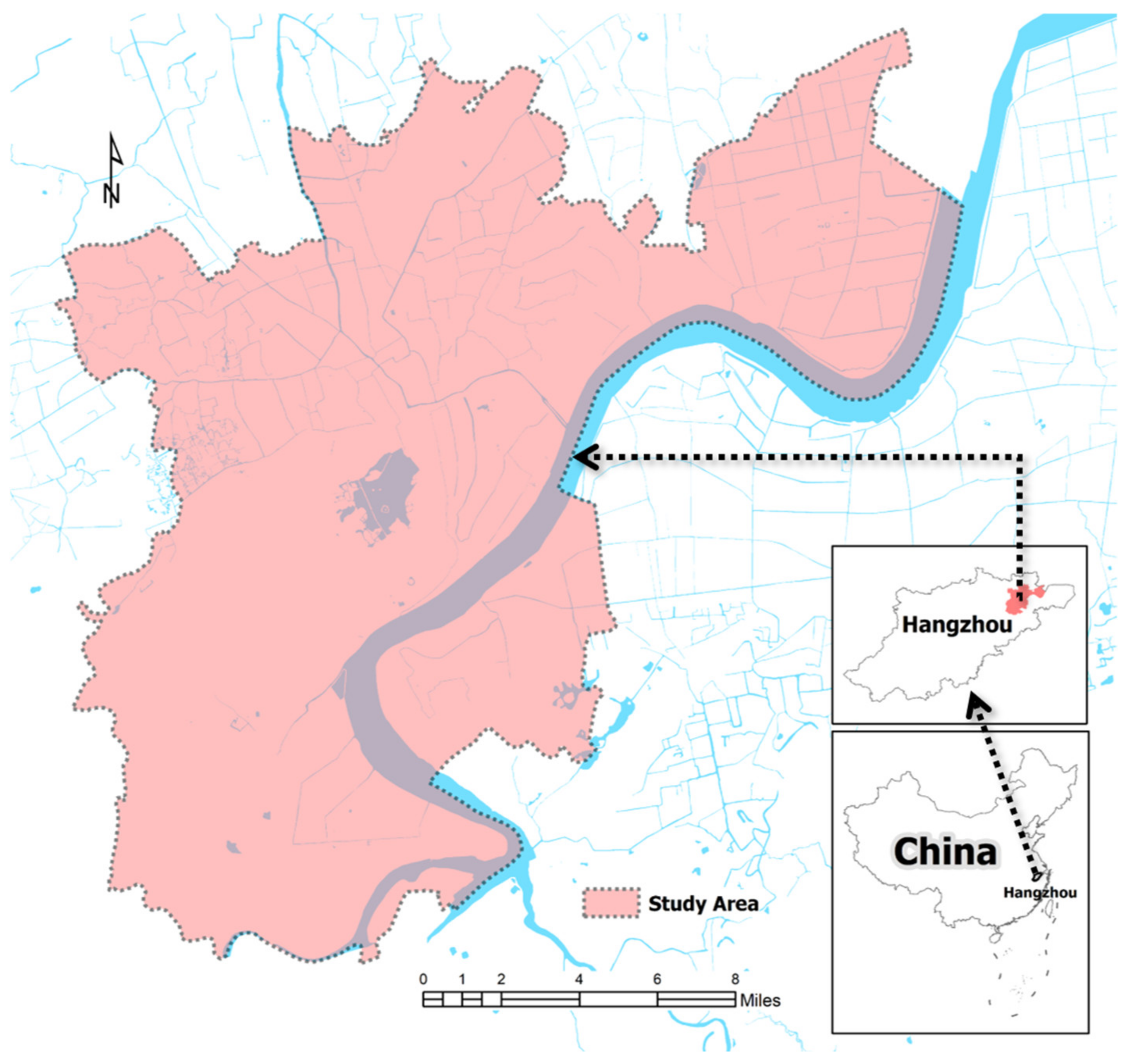
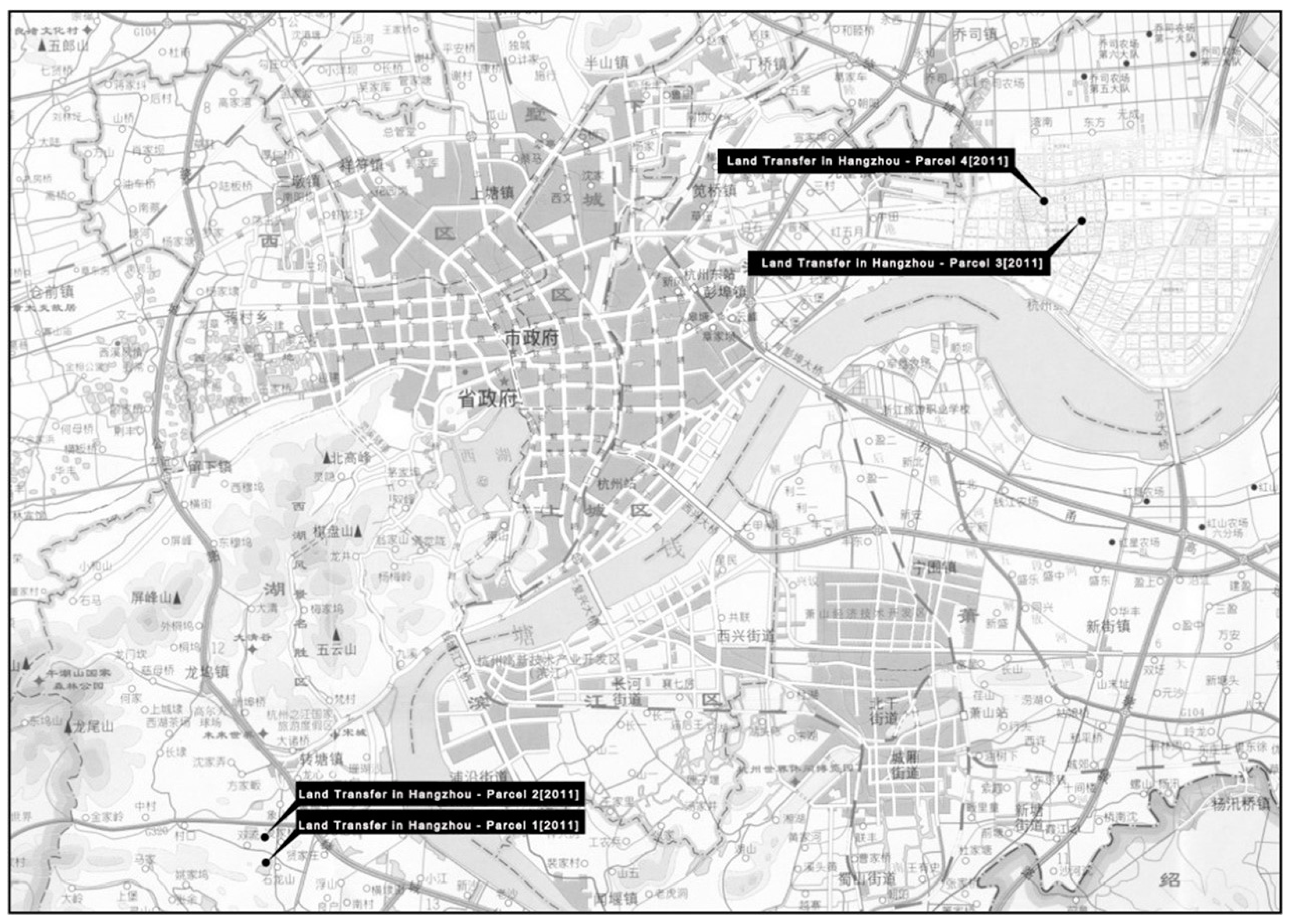
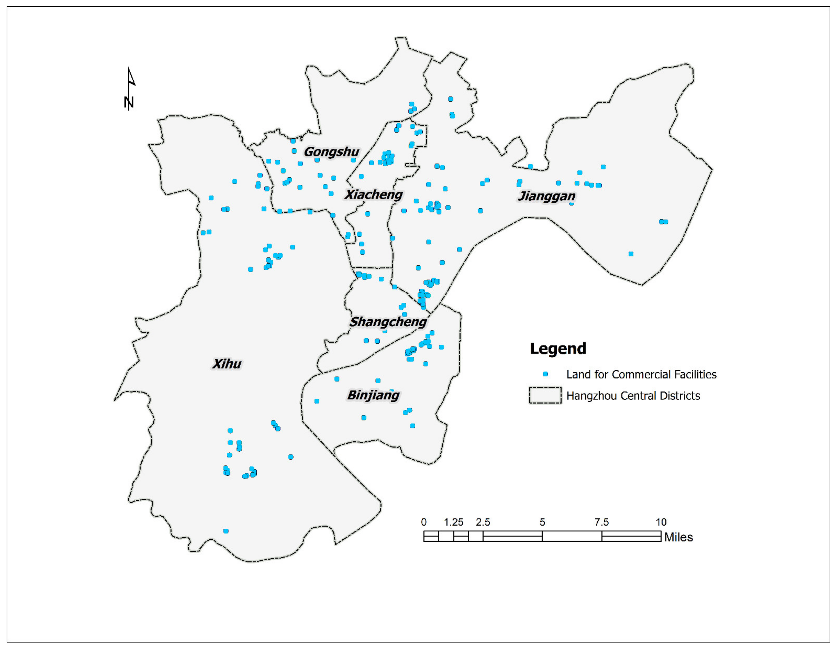
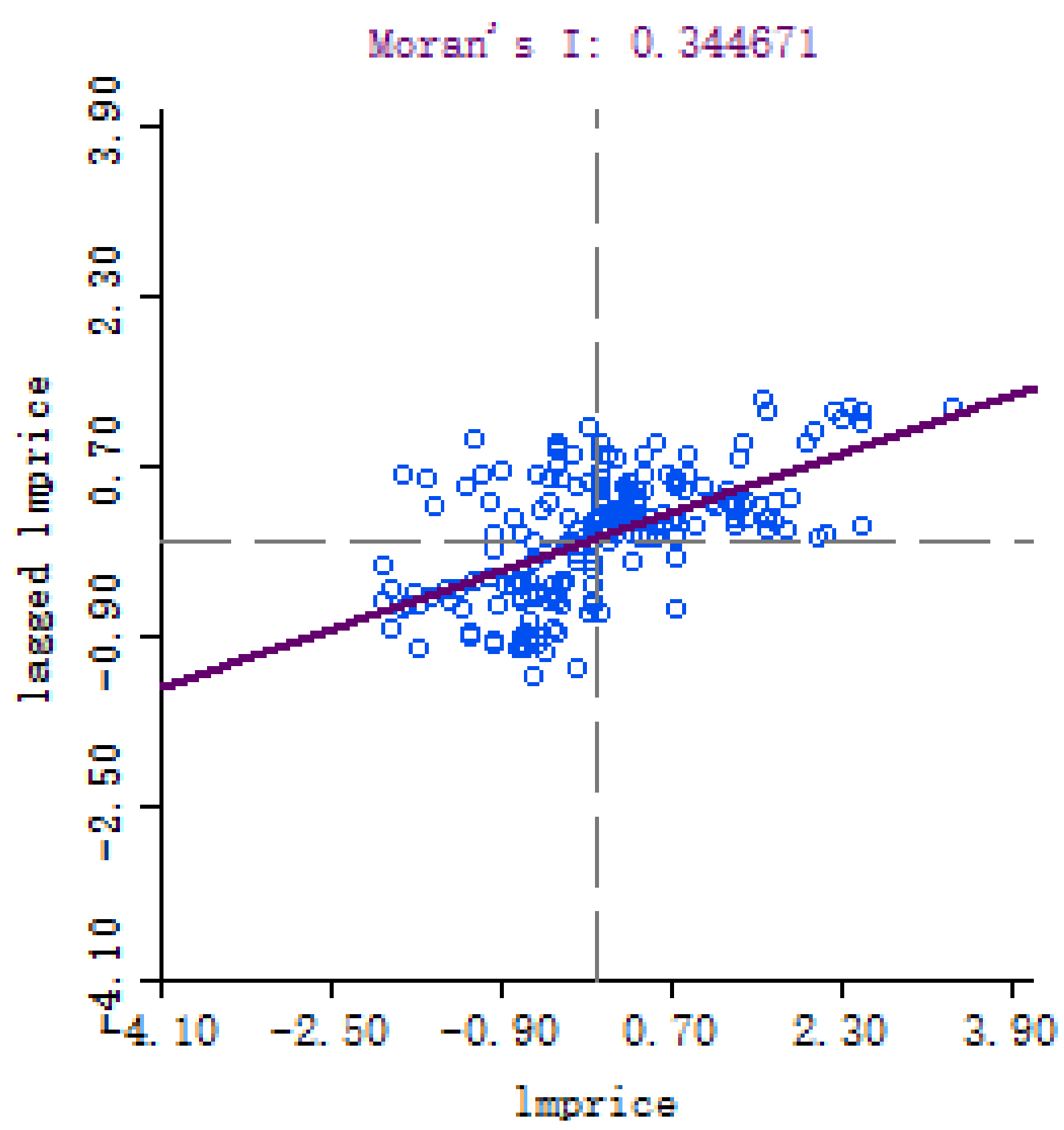
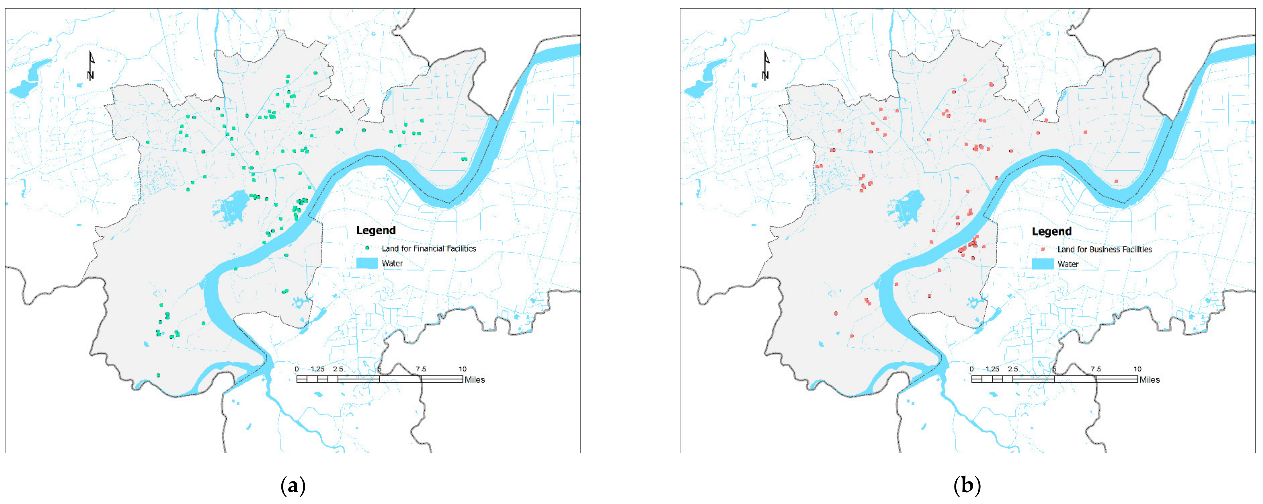
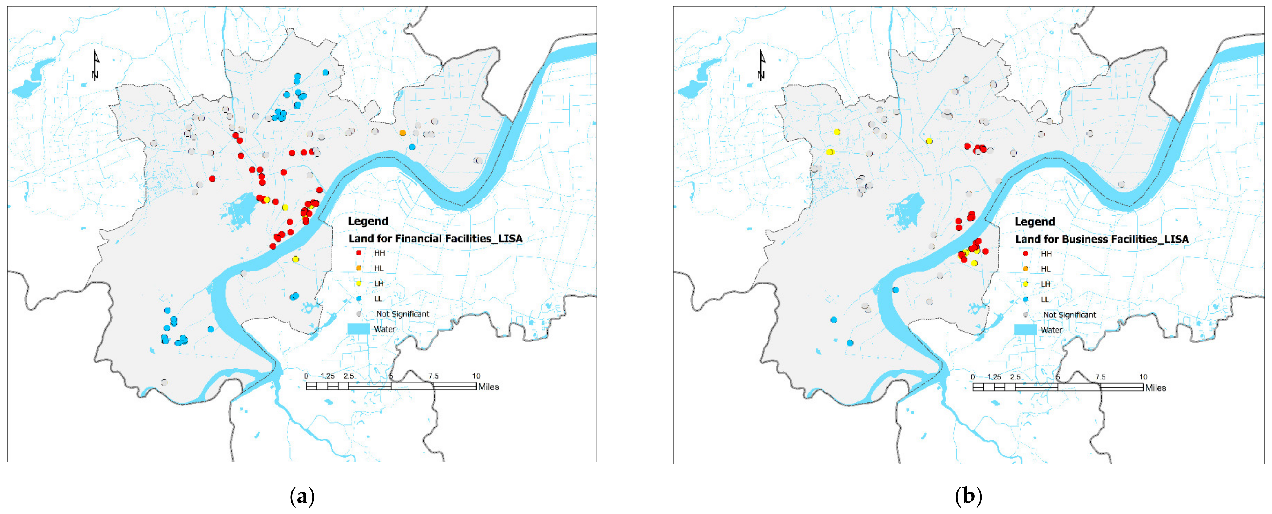
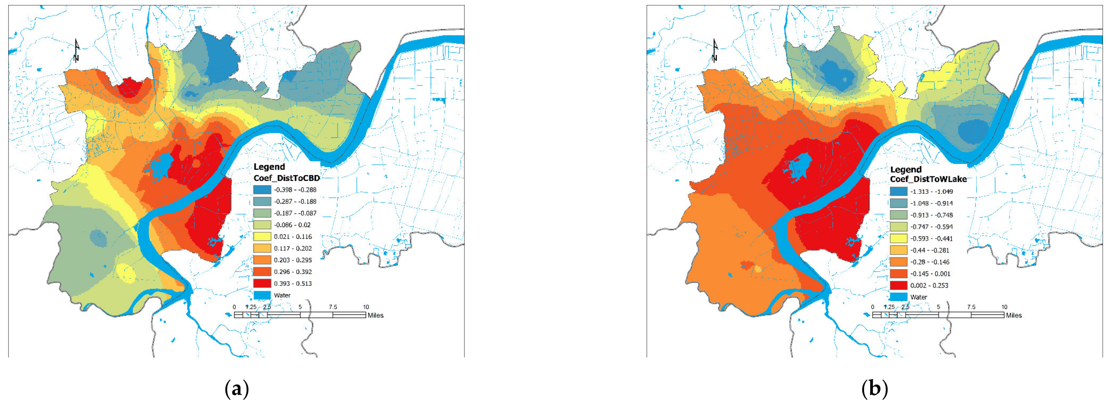
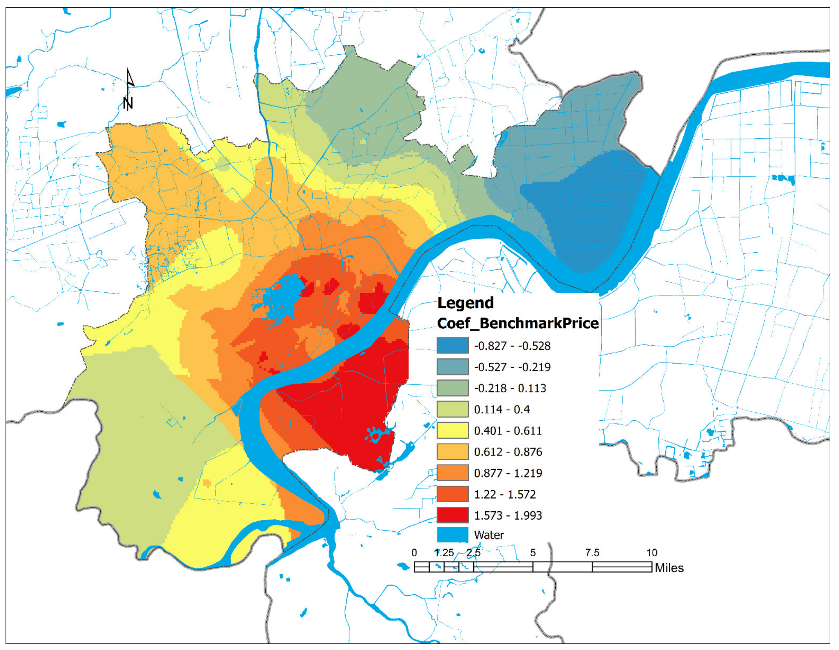
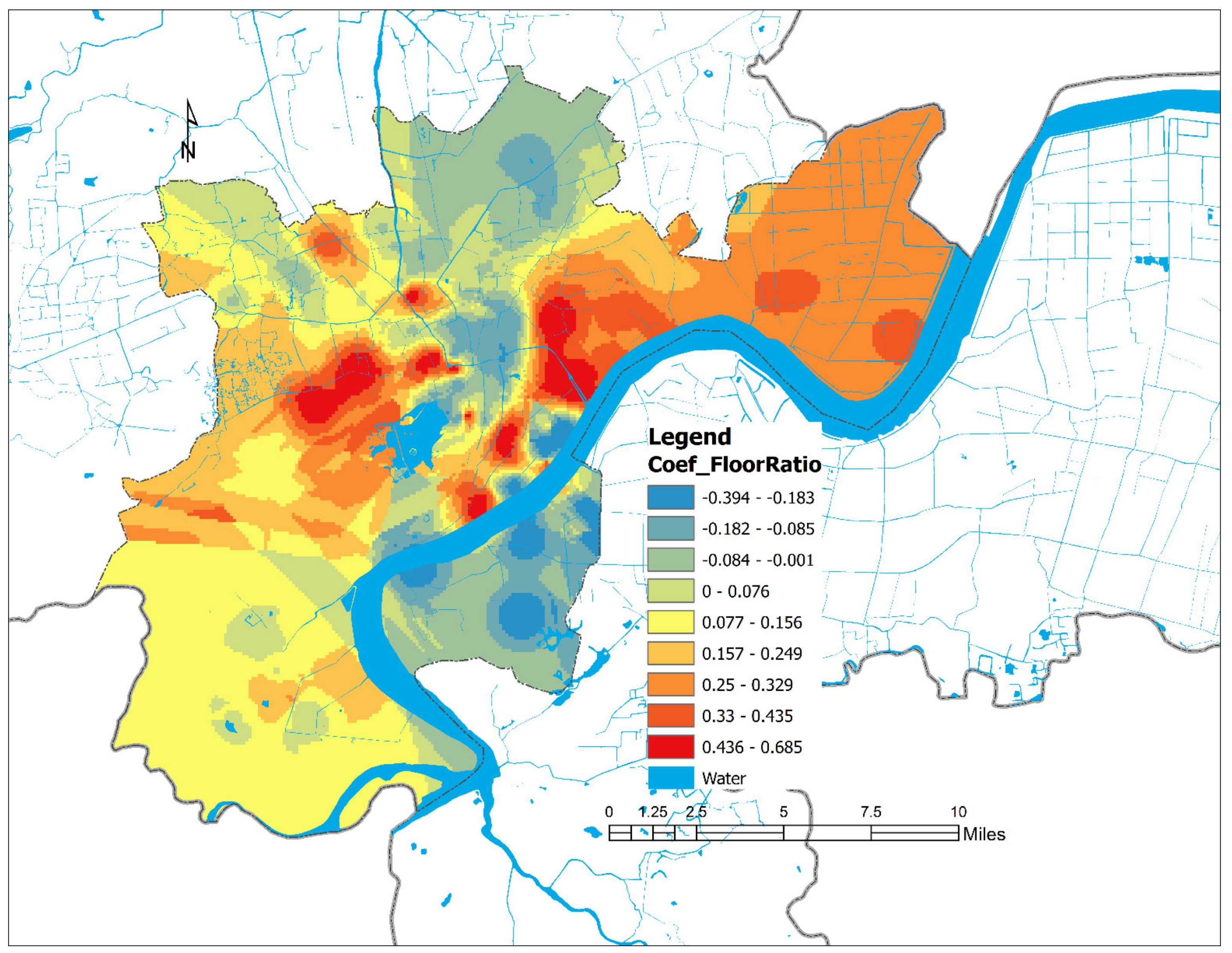
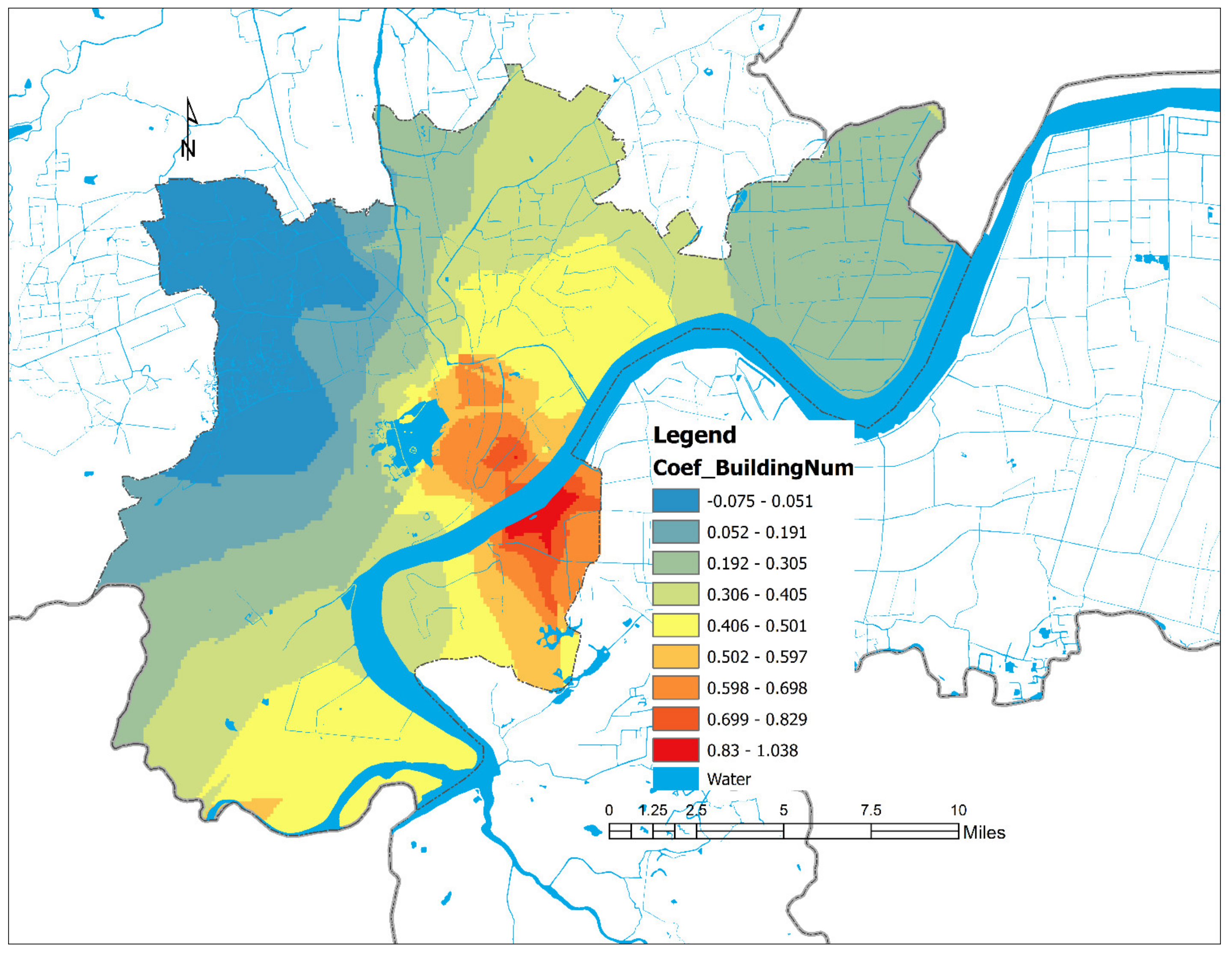
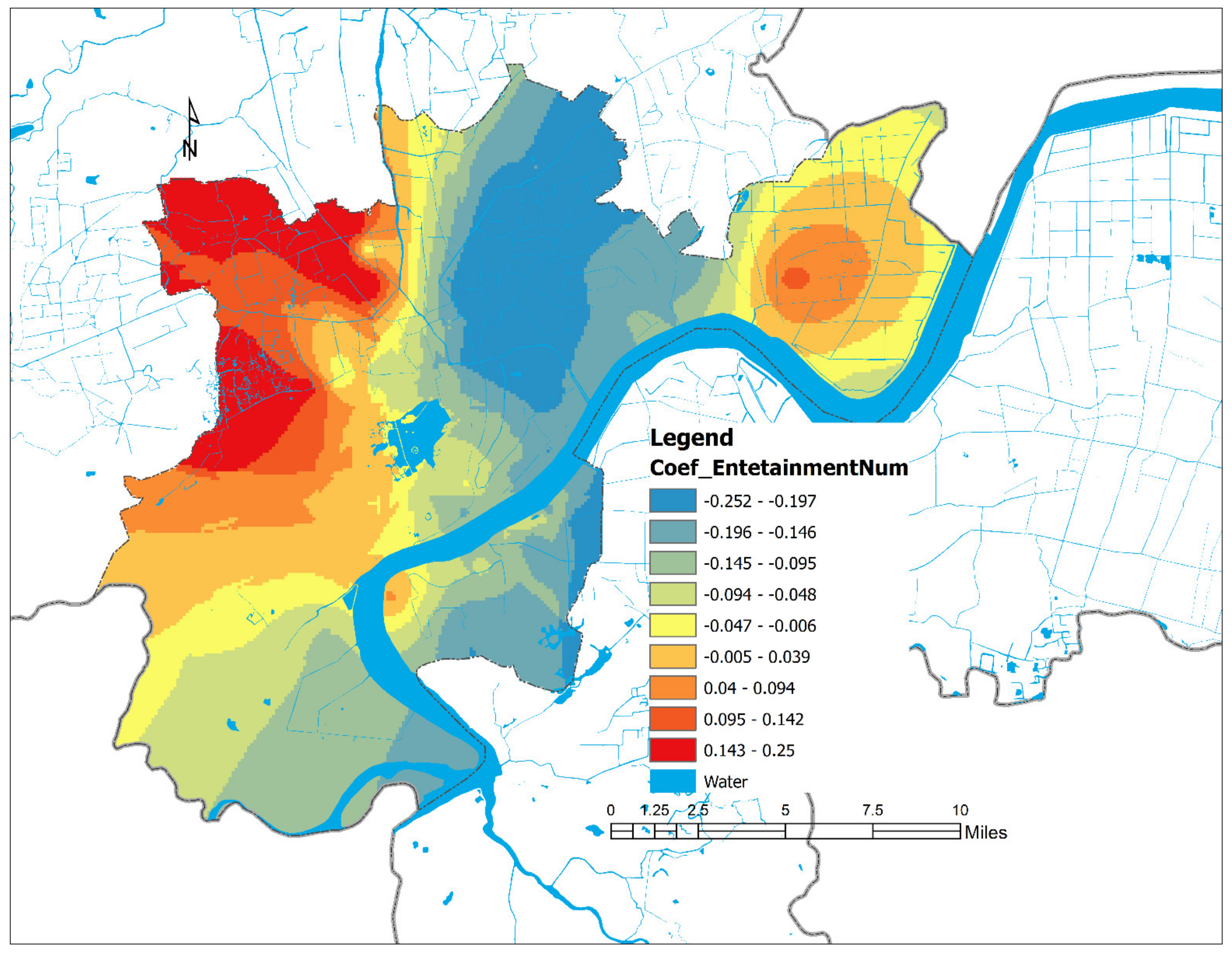
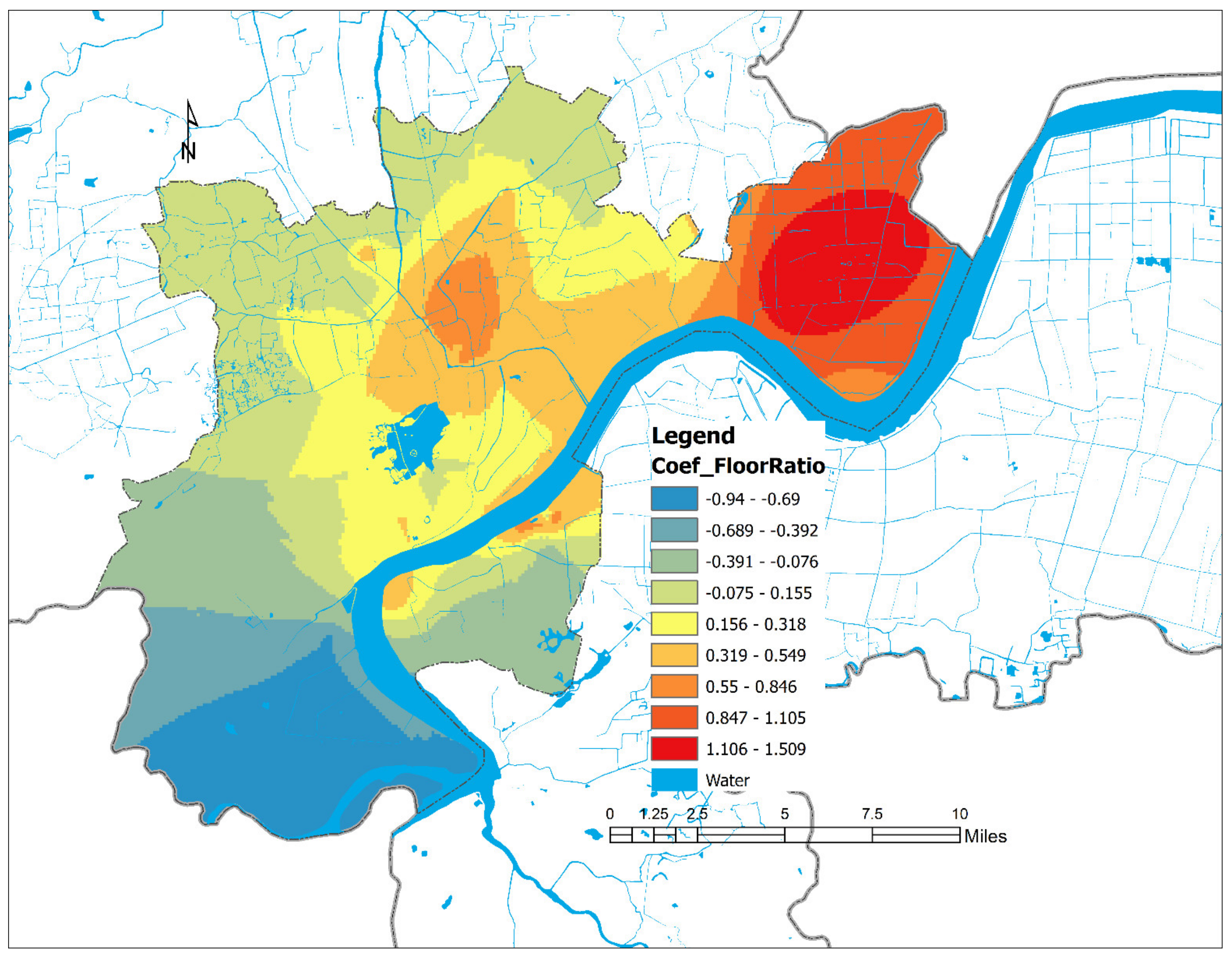
Table 1.
Factors affecting the spatiotemporal evolution of commercial land prices in the main urban areas of Hangzhou.
Table 1.
Factors affecting the spatiotemporal evolution of commercial land prices in the main urban areas of Hangzhou.
| Factor Type | Influencing Factors | Impact Factor |
|---|---|---|
| Geographical factor | Location centrality | CBD1: Distance from Wulin CBD |
| CBD2: Distance from Hubin CBD | ||
| CBD3: Distance from Qianjiang CBD | ||
| Traffic accessibility | SD: Distance from train station | |
| BD: Distance from bus stop | ||
| AD: Distance from airport | ||
| BUSN: Number of bus stops | ||
| Business agglomeration | BUN: Number of surrounding office buildings | |
| Neighborhood factor | Socioeconomic level | EL: Block commercial economic proportion |
| PL: Land price level of the block | ||
| Completeness of living service facilities | EN: Number of surrounding recreational facilities | |
| STD: Number of car parks | ||
| GN: Administrative agencies | ||
| HSD: Distance from the nearest college | ||
| Plot characteristic factor | Parcel area | AR: Parcel area |
| Frontage | RD: Frontage situation | |
| Plot ratio | FRO: Parcel plot ratio |
Table 2.
Statistics on the number of sample points for commercial land transactions in Hangzhou.
| Year | Shangcheng District | Xiacheng District | Jianggan District | Gongshu District | Xihu District | Binjiang District | Subtotal |
|---|---|---|---|---|---|---|---|
| 2006 | 2 | 4 | 2 | 3 | 3 | 14 | 28 |
| 2007 | 6 | 7 | 19 | 4 | 4 | 4 | 44 |
| 2008 | 0 | 5 | 7 | 2 | 5 | 7 | 26 |
| 2009 | 5 | 15 | 10 | 3 | 6 | 3 | 42 |
| 2010 | 1 | 2 | 16 | 7 | 7 | 0 | 33 |
| 2011 | 3 | 5 | 11 | 2 | 5 | 4 | 28 |
| 2012 | 3 | 1 | 15 | 5 | 14 | 4 | 42 |
| 2013 | 2 | 2 | 14 | 7 | 12 | 3 | 40 |
| 2014 | 2 | 0 | 12 | 3 | 7 | 3 | 27 |
| 2015 | 0 | 1 | 0 | 6 | 6 | 1 | 14 |
| Total | 24 | 42 | 106 | 42 | 69 | 43 | 324 |
Table 3.
Design of the corresponding attribute field of the graph database.
| Field Name | Data Type | Description |
|---|---|---|
| ID | Integer | Sample serial number, unique code |
| Serial Number | Integer | Sample data original encoding |
| Parcel name | Character (10) | Hangzhou Land Bureau Reserve Center Number |
| Transfer area | Floating point | Sample land area, unit: square meters |
| Planned building area | Floating point | Sample land planning area, unit: square meters |
| Total Transfer Price | Floating point | Sample land transfer total price, unit: Yuan |
| Land Location | Integer | Location of sample points: 1-Shangcheng District; 2-Xiacheng District; 3-Jianggan District; 4-Gongshu District; 5-Xihu District; 6-Binjiang District |
| Four parcels of land | Character (50) | Description of four parcels of sample plot |
| Transferee | Character (20) | Sample unit bidding unit name |
| Current features | Character (20) | Name of surface architecture in 2015 (incomplete) |
| Development Status | Integer | Development status of sample plot in 2015:1- completed; 2- under construction; 3 - did not start |
| Benchmark land price | Integer | Benchmark land price class |
| Unit price | Floating point | The current transaction unit price of the modified sample plot, unit: Yuan/m2 |
| Floor price | Floating point | The current transaction floor price of the modified sample plot, unit: Yuan/m2 |
| Plot ratio | Floating point | Upper limit of the plot ratio of the sample points |
| Transfer data | Date | Sample point transfer date |
| Distance from city main road | Floating point | The shortest straight line distance between the sample point and the city’s main road, unit: meter |
| Distance from passenger train station | Floating point | The shortest straight line distance between the sample point and the railway station, unit: meter |
| Distance from passenger bus station | Floating point | The shortest straight line distance between the sample point and the bus station, unit: meter |
| Distance from airport | Floating point | The shortest straight line distance between the sample point and the airport, unit: meter |
| Distance from CBD | Floating point | The shortest straight line distance between the sample point and the CBD, unit: meter |
| Distance from West Lake | Floating point | The shortest straight line distance between the sample point and the West Lake, unit: meter |
| Distance from the Qiantang River | Floating point | The shortest distance between the sample point and Qiantang River, unit: meter |
| X coordinate | Floating point | Cartesian coordinates converted by latitude and longitude, obtained by CentroidX (Obj) |
| Y coordinate | Floating point | Cartesian coordinates converted by latitude and longitude, obtained by CentroidY (Obj) |
Table 4.
Classification table of urban land use in Hangzhou in 2005.
| Land Category | Meaning |
|---|---|
| Commercial land | Commercial land, such as shopping malls, supermarkets, trade, services, finance, securities, trusts, futures, insurance, gas stations, hotels, resorts, restaurants, tourism, golf courses, entertainment, telecommunications business sites, etc. |
| Comprehensive land | Comprehensive land, such as offices, office buildings, education, science and technology, culture, health, sports and operational parking lots, and operational storage (including supporting warehouses for shopping malls, supermarkets, and warehouses for external lease) |
| Residential land | Various residential land (including land for common residential, apartments, and villas) |
| Industry land | Land for industry, warehousing, transportation, communications (ancillary facilities), water supply, drainage, power supply, heating, gas supply, sanitation, maintenance of public facilities, etc. |
| Other land | Land outside the above range shall be determined by the Hangzhou Land and Resources Bureau according to the actual situation. |
Table 5.
Comprehensive land price index of Hangzhou from 2006 to 2015.
| Year | 2006 | 2007 | 2008 | 2009 | 2010 | 2011 | 2012 | 2013 | 2014 | 2015 |
|---|---|---|---|---|---|---|---|---|---|---|
| Land price index | 140 | 148 | 149 | 148 | 162 | 173 | 179 | 180 | 192 | 205 |
Table 6.
Estimated global Moran’s I index of commercial land prices in Hangzhou’s main district from 2006 to 2015.
Table 6.
Estimated global Moran’s I index of commercial land prices in Hangzhou’s main district from 2006 to 2015.
| Research Data | Moran’s I | Z | P | |
|---|---|---|---|---|
| Commercial land prices | 0.4540 | −0.0046 | 12.8066 | 0.0000 |
Table 7.
Global Moran’s I index estimated by commercial subdivision land prices in the main district of Hangzhou.
Table 7.
Global Moran’s I index estimated by commercial subdivision land prices in the main district of Hangzhou.
| Commercial Subdivision Category | Moran’s I | Z Value | P Value | |
|---|---|---|---|---|
| Commercial land category 1 | 0.4734 | −0.0008 | 17.0323 | 0.0000 |
| Commercial land category 2 | 0.3403 | −0.0028 | 10.42 | 0.0000 |
Table 8.
Statistics of goodness of fit of different models.
| Model | R2 | RSS | AIC |
|---|---|---|---|
| GTWR | 0.7903 | 16.7087 | 147.7910 |
| TWR | 0.7801 | 17.5158 | 151.2080 |
| GWR | 0.6642 | 26.7586 | 223.8970 |
| OLS | 0.5127 | 38.6677 | 255.1580 |
| The increase in GTWR/OLS | 0.2776 | 21.9590 | 107.3670 |
| The increase in GTWR/GWR | 0.1261 | 10.0499 | 76.1060 |
| The increase in GTWR/TWR | 0.0102 | 0.8071 | 3.4170 |
Table 9.
OLS model statistical diagnostic table of Commercial subdivision.
| Inspection Object | R2 | AIC | RSS | F-Statistics | P-Value |
|---|---|---|---|---|---|
| Commercial land category 1 | 0.7066 | 124.311 | 13.843 | 11.5594 | 0.0000 |
| Commercial land category 2 | 0.7395 | 47.118 | 14.935 | 8.2314 | 0.0000 |
Table 10.
Statistically significant factor results of the commercial land category 1 and commercial land category 2 land price OLS model.
Table 10.
Statistically significant factor results of the commercial land category 1 and commercial land category 2 land price OLS model.
| Influencing Factors | Commercial Land Category 1 | Commercial Land Category 2 | ||||||
|---|---|---|---|---|---|---|---|---|
| Coefficient | Standard Deviation | t-Statistics | p-Value | Coefficient | Standard Deviation | t-Statistics | t-Probability | |
| Constant term | −453.222 | 549.7086 | −0.8245 | 0.4117 | −983.0217 | 637.74 | −1.5414 | 0.1287 |
| CBD1 | −0.2259 * | 0.1251 | −1.8045 | 0.0794 | −0.2625 | 0.2651 | −0.9899 | 0.3263 |
| CBD2 | −0.0596 | 0.0813 | −0.732 | 0.4659 | −0.0473 | 0.0885 | −0.5343 | 0.5951 |
| CBD3 | 0.2904 ** | 0.0857 | 3.3898 | 0.001 | −0.0682 | 0.1352 | −0.5044 | 0.6158 |
| AD | 0.4613 | 0.825 | 0.5591 | 0.5774 | 0.9706 | 0.7358 | 1.3191 | 0.1923 |
| BD | 0.0164 | 0.078 | 0.2322 | 0.5456 | −0.0688 | 0.0764 | −0.9227 | 0.36 |
| BUN | 0.0637 | 0.105 | 0.6064 | 0.5333 | 0.2431 ** | 0.1108 | 2.1948 | 0.0321 |
| BUSD | 0.0014 | 0.1223 | −0.6252 | 0.986 | 0.068 | 0.0954 | 0.6489 | 0.5189 |
| AR | −0.1430 ** | 0.0418 | −2.9714 | 0.0037 | −0.0451 | 0.053 | −0.8512 | 0.3981 |
| PL | 0.6183 ** | 0.2223 | 2.781 | 0.0065 | 0.2449 | 0.1921 | 1.2747 | 0.2075 |
| EN | −0.1218 * | 0.0625 | −1.9468 | 0.0544 | −0.1148 * | 0.0604 | −1.8992 | 0.0625 |
| FRO | 0.2196 * | 0.123 | 1.7857 | 0.0773 | 0.3033 ** | 0.1126 | 2.6974 | 0.0091 |
| GN | −0.0264 | 0.0604 | −0.4373 | 0.6628 | −0.1091 | 0.0065 | −1.6646 | 0.1014 |
| EL | 0.083 | 0.1497 | 0.5557 | 0.5797 | 0.1951 | 0.1604 | 1.2186 | 0.2227 |
| RD | −0.0162 | 0.0804 | −0.2016 | 0.8407 | −0.047 | 0.0885 | −0.5343 | 0.5951 |
| SD | −0.0399 | 0.0654 | −0.2147 | 0.8302 | −0.0077 | 0.0597 | −1.302 | 0.198 |
| STD | −0.0399 | 0.0919 | −0.4339 | 0.6653 | 0.1095 | 0.1144 | 9556 | 0.3432 |
| HSD | 0.0248 | 0.0604 | 0.472 | 0.638 | 0.0164 | 0.0357 | 0.3069 | 0.7601 |
| POINT_X | 10.886 | 15.0401 | 0.5319 | 0.5954 | 35.5291 * | 20.4364 | 1.7385 | 0.0874 |
| POINT_Y | 16.3086 | 30.3465 | 0.4175 | 0.6768 | 21.0141 | 45.0903 | 0.5769 | 0.5662 |
| Time | 6.2066 ** | 1.3896 | 6.0026 | 0.0088 | 11.7271 ** | 2.0518 | 5.7154 | 0 |
Note: Values marked with * and ** passed the statistical test with statistical values of 10%, 5%, and 1%, respectively.
Table 11.
GTWR goodness of fit statistics of different commercial land types.
| Commercial Subdivision | R2 | RSS | AIC |
|---|---|---|---|
| Commercial land category 1 | 0.8623 | 16.5496 | 71 |
| Commercial land category 2 | 0.7644 | 14.5258 | 57 |
Table 12.
GTWR regression results of commercial land category 1.
| Impact Factor | Minimum Value | Maximum Value | Mean Value | Median Value |
|---|---|---|---|---|
| AR | −0.2961 | 0.0873 | −0.1377 | −0.1465 |
| FRO | −0.4 | 0.7 | 0.075 | 0.026 |
| EN | 0.359 | 0.1751 | −0.1323 | 0.13468 |
| PL | −0.829 | 1.9907 | 0.7994 | 0.7445 |
| CBD2 | −1.3431 | 0.2568 | −0.2385 | −0.132 |
| CBD3 | −0.3958 | 0.51655 | 0.1545 | 0.2 |
Table 13.
GTWR Regression results of commercial land category 2.
| Minimum Value | Maximum Value | Mean Value | Median Value | |
|---|---|---|---|---|
| FRO | −0.94112 | 1.5131 | 0.2602 | 0.3122 |
| EN | −0.2529 | 0.253 | −0.89 | −0.1075 |
| BUN | −0.197 | 1.2499 | 0.4444 | 0.3993 |
Publisher’s Note: MDPI stays neutral with regard to jurisdictional claims in published maps and institutional affiliations. |
© 2021 by the authors. Licensee MDPI, Basel, Switzerland. This article is an open access article distributed under the terms and conditions of the Creative Commons Attribution (CC BY) license (http://creativecommons.org/licenses/by/4.0/).
Share and Cite
MDPI and ACS Style
Garang, Z.; Wu, C.; Li, G.; Zhuo, Y.; Xu, Z. Spatio-Temporal Non-Stationarity and Its Influencing Factors of Commercial Land Price: A Case Study of Hangzhou, China. Land 2021, 10, 317. https://doi.org/10.3390/land10030317
AMA Style
Garang Z, Wu C, Li G, Zhuo Y, Xu Z. Spatio-Temporal Non-Stationarity and Its Influencing Factors of Commercial Land Price: A Case Study of Hangzhou, China. Land. 2021; 10(3):317. https://doi.org/10.3390/land10030317
Chicago/Turabian StyleGarang, Zhuoma, Cifang Wu, Guan Li, Yuefei Zhuo, and Zhongguo Xu. 2021. "Spatio-Temporal Non-Stationarity and Its Influencing Factors of Commercial Land Price: A Case Study of Hangzhou, China" Land 10, no. 3: 317. https://doi.org/10.3390/land10030317
Note that from the first issue of 2016, this journal uses article numbers instead of page numbers. See further details here.