The Resilient Recurrent Behavior of Mediterranean Semi-Arid Complex Adaptive Landscapes
by
 , , ,
, , ,
Irene Petrosillo
1, 
Donatella Valente
1,*,
Christian Mulder
2,
Bai-Lian Li
3,
K. Bruce Jones
4 and
Giovanni Zurlini
1 1
Landscape Ecology Laboratory, Department of Biological and Environmental Sciences and Technologies, ECOTEKNE, University of Salento, 73100 Lecce, Italy
2
Department of Biological, Geological and Environmental Sciences, University of Catania, 95131 Catania, Italy
3
Department of Botany and Science & Plant Sciences, University of California, Riverside, CA 92521, USA
4
Desert Research Institute, Las Vegas, NV 89119, USA
*
Author to whom correspondence should be addressed.
Land 2021, 10(3), 296; https://doi.org/10.3390/land10030296
Submission received: 25 January 2021
/
Revised: 18 February 2021
/
Accepted: 10 March 2021
/
Published: 13 March 2021
(This article belongs to the Section Landscape Ecology)
Abstract
:Growing external pressures from human activities and climate change can exacerbate desertification, compromising the livelihoods of more than 25% of the world’s population. The dryland mosaic is defined by land covers that do not behave similarly, and the identification of their recurring or irregular changes over time is crucial, especially in areas susceptible to become desertified. To this aim, the methodological approach of this research is based on the integration of non-linear data analysis techniques, such as recurrence plots (RPs) and recurrence quantification analysis (RQA), applied to the Enhanced Vegetation Index (EVI), which is a functional ecological proxy of above ground net primary production. The research exploits the recurring change detected in vegetation cover over time to gauge the predictable (resilient) behavior of the EVI as well as its chaoticity in a semi-arid Mediterranean region (Apulia, Italy). Interestingly, the results have shown the spatial rendering of recurrence variables, confirming the well-known hot spots of soil degradation and desertification taking place in the region, which are characterized by greater EVI chaoticity, but they have also identified new potential candidate sites. As a result, the susceptibility to land degradation, as measured by the EVI-RQA approach, can help in measuring land desertification with evident operational benefits for landscape planning. The novelty of the research lies in the spatially explicit identification of resilient and less resilient areas to desertification that can support the definition of more targeted interventions and conservation priorities for better planning and sustainable management of Mediterranean drylands.
1. Introduction
Complex adaptive systems [1] such as socio-ecological landscapes (SELs) [2,3] show generally nonstationary and complex behavior and are usually assumed to respond smoothly to gradual change in climate, habitat fragmentation or exploitation. Such a condition can be sporadically interrupted by abrupt shifts towards a radically different regime [4]. Resilient SELs can adapt the behavior of the system (adaptability) to changes in external drivers and internal processes and remain in the current domain of stability or basin of attraction [2].
Research and practice in SELs are increasingly converging on a series of a few general lessons as they apply to sustainable development in drylands [5]: (1) the need to adopt an integrated approach, (2) a greater awareness of slowly changing conditions, (3) the recognition of non-linear processes since dryland systems are not in equilibrium, and therefore often show multiple ecological and social states, and (4) cross-scale interactions must be expected. In our approach, we have tried to address these lessons and to synergize them in the analytical techniques adopted.
Land degradation has been defined by the Millennium Ecosystem Assessment (MEA) as “a persistent net loss of capacity to yield provisioning, regulating, and supporting ecosystem services” [6]. The MEA refers to desertification as the same degradation process in drylands (i.e., semi-arid, arid and dry sub-humid zones). In this context, landscape services [7] directly or indirectly sustain the quality of human life and are provided by physical structures and processes called “supporting services” [6,8], among which the above-ground net primary production (ANPP) is a key-controlling factor determining most of the landscape service provisioning capacities [6]. Such essential supporting services influence the entire ecosystem functioning, governing most of provisioning and regulating services (e.g., food, water cycling and regulation, nutrient cycling) and even some cultural services, which tend to shift in concert with it [8,9,10]. Thus, a reduction in ANPP at a site is often viewed as land degradation [5] that, if exacerbated, can lead to a state of irreversible desertification [11]. As such, efforts to reduce the risk of undesirable state transitions such as land degradation and desertification should include an assessment of gradual or irregular changes or transitions in ANPP, rather than merely trying to control disturbances [4].
Vegetation cover is the primary determinant of SEL mosaics and is quite responsive to land cover transformations at all scales, as all climate changes and anthropogenic influences have a spatial outcome. Therefore, current integrated approaches to monitoring and assessing land degradation and desertification (LDD) often rely on two technological aspects: (1) the remote sensing of vegetation cover and (2) the analysis of satellite data (vegetation indices) through specific tools, such as geographic information systems (GIS) and time series analysis techniques [12].
However, while most of the integrated approaches to assess LDD focus mainly on the selection of one or few vegetation indices and try to link the generated spatial information with a variety of environmental and socio-economic data in a single framework, less emphasis is placed on the adequacy and effectiveness of time series analysis techniques to extract useful information from the analysis of time series behavior [12,13].
Since natural or human-dominated processes can have a distinct recurrent behavior, e.g., periodicities (as seasonal or Milankovich cycles), but also irregular cycles like ENSO (the El Niño-Southern Oscillation), the study of recurrence is becoming essential as it is a fundamental property of deterministic dynamical systems to be studied, and it is also typical of non-linear or chaotic systems [14]. It allows the measurement of resilience in terms of stability/predictability, which can be defined as the probability of a system’s multiple states to persist and recur [15].
In this perspective, the purpose of this research is to demonstrate the effectiveness of the recurrence quantification analysis (RQA) [14] to provide for the region of interest (a) the estimate of the recurring resilience-related variables from the behavior of the Enhanced Vegetation Index (EVI) time series over the entire 14-year period, (b) the spatialization of the recurrence variables on the regional scale to identify hot spots with different stability/predictability as well as chaoticity of space-time functional dynamics because of climate change and/or water scarcity or human activities, and (c) the validation of this mapping with the confirmation of the well-known land degradation and desertification hot spots in the region as well as the identification of new sites as potential candidates to become desertified. To this aim, the available functional dynamics of vegetation covers in a Mediterranean semi-arid region have been analyzed in terms of possible recurrent and, therefore, predictable behaviors through: (a) time series of the Enhanced Vegetation Index (EVI), which is an ecological functional proxy of ANPP [16,17] and its changes can reflect the effects of changes associated with climate, land conversion, and farming practices as well as drought and fire, and (b) the use of non-linear data analysis techniques such as recurrence plots (RPs) and recurrence quantification analysis (RQA) [14] applied to the average EVI time series extracted from satellite multitemporal images.
It is interesting to note that these techniques, unlike those normally used, do not involve any manipulation of the original data and are fully independent from binding hypotheses and signal transformations. They are also applicable to relatively short time series and provide resilience-related recurrence variables that refer to stability/predictability and, conversely, chaoticity (the condition of being chaotic) [14]. We argue that the greater the stability/predictability of time series belonging to a land cover class, as shown by the recurrence of states within preferred bounds (adaptability), the higher the likelihood that such a class will be resilient to contagious and non-contagious stress, often showing, but not necessarily, a regular recurrent behavior [18]. Conversely, all the unfavorable biophysical factors that promote desertification in Mediterranean drylands, such as erratic precipitation (mainly during the winter), high summer temperatures with frequent drought events, poor and erodible soils, extensive deforestation with frequent wildfires and land abandonment [19], are expected to reverberate on the chaotic EVI temporal behavior, as highlighted by RP-RQA.
2. Materials and Methods
2.1. Study Area
Dryland landscapes are, in general, characterized by water scarcity and high climate variability, with strong weather extremes. In the Mediterranean basin, drylands are characterized by a strong multifunctionality since they coevolved with humans for millennia [20,21]. These landscapes are characterized by a progressive land degradation with the consequent loss of crucial services such as food production, soil quality regulation, water regulation, climate regulation, identity value, and people’s sense of belonging to semi-arid landscapes and their associated recreational services [22,23].
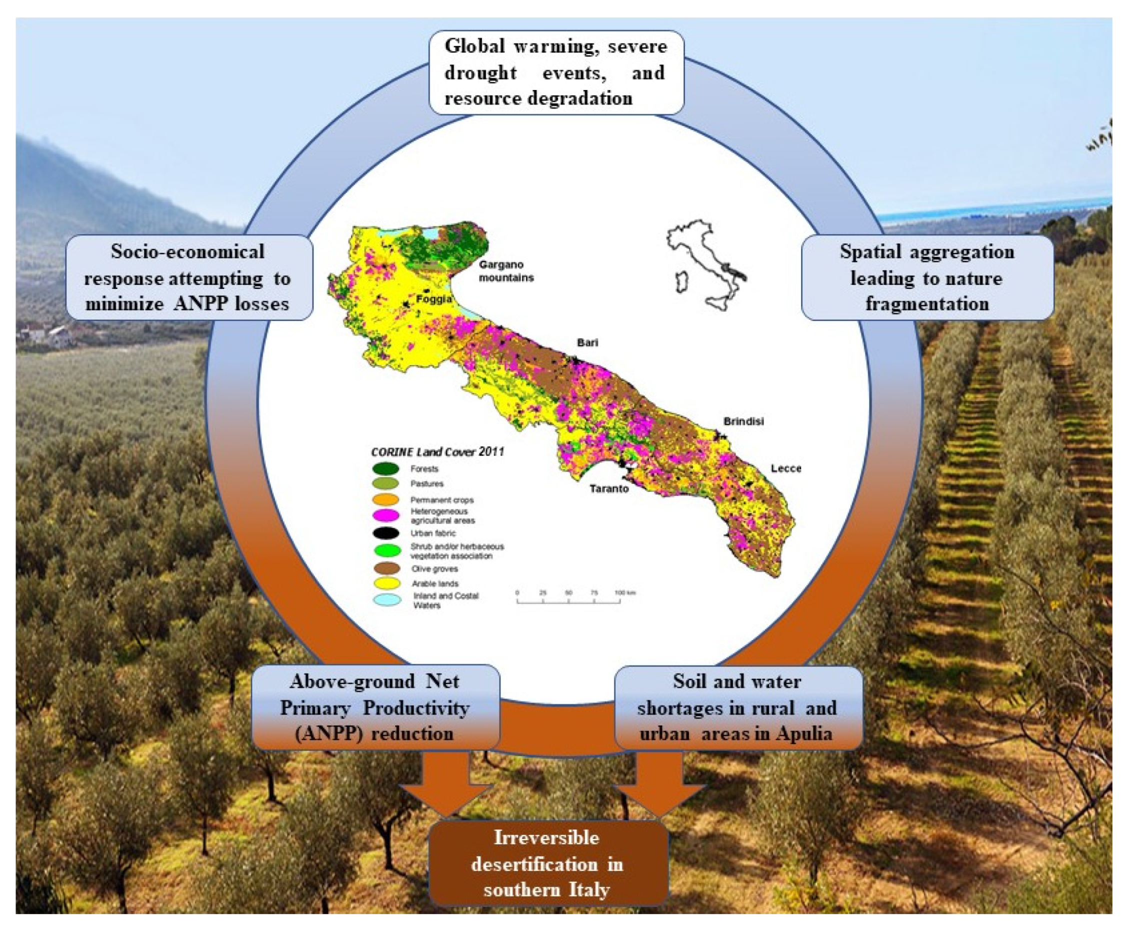
The study area (Figure 1) represents a typical Mediterranean semi-arid region [24], where more than 82% of the area is constituted by agroecosystems, critically dependent on water availability [25], where extensive forest clearances have occurred since the middle Holocene [26,27], slowly leading to desertification [28,29].
A robust and consistent picture of climate change over the Mediterranean has emerged, consisting of both a pronounced decrease in precipitation, especially in the summer season, and a temperature increase, with its maximum in the summer leading to an increased frequency of high-temperature events [30,31]. The main landscape changes responsible for land desertification are given by the merging of arable lands [32], a contraction of vineyards, and the expansion of olive groves, plantations, and urban areas, with large increases in energy use, water consumption, and fertilizer applications, leading to extensive biodiversity loss (Figure 1) [33]. As a result, the main vulnerability of the region relates to its persistent water scarcity and its water budget deficit (about 350 mm/year), requiring regular water imports from nearby regions and forcing the exploitation of aquifers [34,35].
The introduction of new farm machinery and strains of cereals and trees, along with the overexploitation of water resources for irrigated agriculture and the extensive application of fertilizers, represent the main socio-economic drivers of soil erosion and LDD in Mediterranean Europe [35] as well as in Apulia [29]. The net irrigation requirements are expected to increase in the next century, with a maximum of 65% for intensive olive groves due to the excessive pumping of groundwater [25]. This will increase water stress by the intensity, extent, timing, and duration of water availability [36] as well salinity intrusion in groundwater, one of the main drivers for the salinization of coastal soils.
The northern and central parts of the region are dominated by arable lands, whereas the central and southern parts of the region are dominated by extensive century-old as well as intensive olive groves, and other rural areas (Figure 1). The few natural habitats are unevenly distributed as forested areas concentrated in the Gargano peninsula, as well as a few remnants of evergreen forests interspersed with olive groves. In addition, natural drylands are present with shrub and/or herbaceous vegetation and permanent pastures (Figure 1), including semi-arid grasslands, garigues, steppes and pastures, all collected here under the name of Grasslands, present in Daunia and Murgia Apennines.
2.2. Materials: Real World Time Series of Vegetation Indices
The normalized difference vegetation index (NDVI) has been widely used over the last few decades in the satellite-based modeling of ANPP for terrestrial vegetation [37,38,39]. However, several limitations have been observed when applying the NDVI index in dry land area research [23,40]; therefore, in this research, the enhanced vegetation index (EVI) [40] was preferred as it has been used in the satellite-based modeling of ANPP [41], is found more linearly correlated with the green leaf area index (LAI) in crop fields [42], is less prone to greenness saturation and has higher robustness to atmospheric conditions and soil background relative to NDVI [13,40,43]. Moreover, perennial and annual vegetation types that green up in deserts at rates and times characteristic for their distinct species can be easily captured by EVI data [44].
Integrated approaches based on time series of vegetation indices have mostly used linear techniques focusing on different aspects of temporal complexity. Recently, the “normalized spectral entropy”, a non-linear analysis, has been developed to describe the degree of regularity (orderliness) and to characterize heterogeneity within an ecological time series based on its power spectrum [18,21,45], pointing to the system’s self-organization strength [46]. However, because of non-stationarity, noise, relatively short time series [47] and frequently complex shapes of recurrent periodicities, more advanced methods are needed for quantifying non-linear dynamics [21,48].
2.3. Methods
The methodology is based on two steps:
First step: satellite data harmonization and cross-correlation with temperature and precipitation.
The Moderate Resolution Imaging Spectroradiometer (MODIS, https://modis.gsfc.nasa.gov/ accessed on 25 June 2018), onboard the NASA Terra and Aqua satellites, provides both NDVI and EVI images with high temporal frequency and medium spatial resolution, allowing us to gauge the continuous flow of ANPP. MODIS EVI images (USGS, https://glovis.usgs.gov/ accessed on 25 June 2018) are already filtered from daily data, although further filtering was necessary to keep the most reliable EVI. To this end, a simple filter (to avoid high drops of EVI between two high EVI values) was applied as in [49], and then, to build the most reliable EVI profile, a simple gap-fill approach has been used to implement the method of Xiao et al. [16,43].
For each pixel belonging to the Apulia region, we extracted EVI time series relative to 323 EVI maximum value composite MODIS images acquired by the two MODIS platforms TERRA and AQUA with a spatial resolution of 250 m (MOD13Q1 v.005 and MYD13Q1 v.005) and with a sampling time (Δt) of 16 days over fourteen years (2000–2014). To facilitate interpretation, EVI time series for each location were associated with land cover classes according to the 2011 4th level CORINE land cover map (https://www.dataset.puglia.it/dataset/uso-del-suolo-2011-uds accessed on 25 June 2018) (Figure 1).
Finally, cross-correlation analyses of EVI with temperature and precipitation were performed on a ten-day basis, acquired from the Italian National Environmental Information System (http://www.sinanet.isprambiente.it/it/sia-ispra accessed on 25 June 2018), and related to six weather stations distributed throughout the Apulia region inside or in proximity to the types of land cover analyzed in this study. This was performed to evaluate how the EVI and associated RAQ metrics were related to precipitation and temperature. Understanding this is central to being able to pull out signals of other perturbations, as well as responses to drought.
Step 2: Recurrence Plots/Recurrence Quantification Analysis.
Recurrence Plots (RPs) and Recurrence Quantification Analysis (RQA) are non-linear time series analysis techniques [14] with growing application in different fields [50,51,52,53,54,55] because of their applicability to relatively short time-series, full independence from constraining assumptions (outliers, linearity, stationarity) and signal transformations (detrending, noise filtering).
In this research, RP-RQA was performed on the average time series of the four main types of land cover (Forests, Olive Groves, Arable Lands, Grasslands) representing 94.2% of the entire Apulia region, with a sampling time of 16 days over fourteen years (2000–2014). The recurrence is the time it takes for the trajectory of an EVI series to return to its original state.
A brief overview of RP and RQA is reported below, but more details of the principles and algorithms can be found in [14,21].
A landscape state consists of state variables describing all the important properties of dynamical systems; therefore, it can be mathematically depicted by a vector
with embedding dimension m and time delay τ.
The temporal evolution of the state is expressed by the phase space trajectory of the dynamical system. Formally, the RP is based on the recurrence matrix:
where N is the number of measured states , i.e., the length of the time series reduced by the number (m − 1) τ; ε is a threshold distance; and ║·║ is a norm, i.e., the spatial distance between two points xi and xj in the phase space trajectory. The choice of m is usually based on counting false nearest neighbors when increasing m and choosing the value of m where the number of false nearest neighbors goes to zero [14]. The delay τ must be selected to minimize the autocorrelations between the time series points, e.g., by using mutual information. The parameter ε is crucial as systems often do not recur exactly but just approximately to a formerly visited state. The appropriate threshold ε can be selected by following three methods, i.e., mean or maximum phase space diameter, recurrence point density, and standard deviation of the observational noise [14].
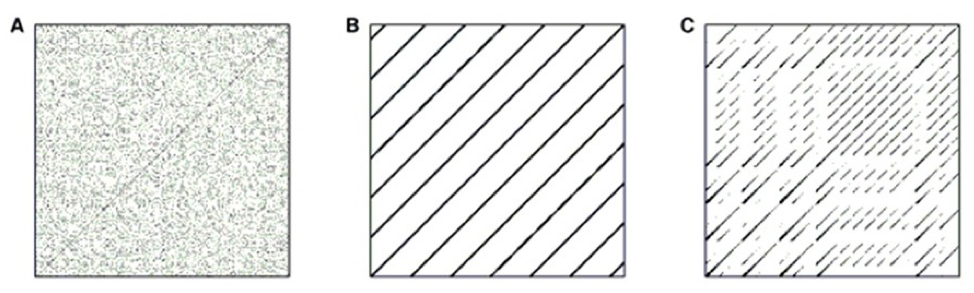
The RP is a graphical representation of this recurrence matrix (Figure 2), where black points represent those time points where the spatial distance between two states and is falling below the threshold ε and, therefore, the system recurs [14,54]. For illustrative purposes, the RPs of three typical synthetic time series (A, B, C) are presented (Figure 2). In particular, the trajectory with regular oscillations (Figure 2B) is the least common in nature, but the possibility given by RQA to analyze more complex but recurrent oscillation trends represents the strength of the RQA approach. Diagonal lines in the RP indicate that the temporal evolution of states is similar at different times and, therefore, can point to deterministic processes; vertical or horizontal lines in the RP indicate that some states do not change or change very slowly for some time and can suggest laminar or persistent states.
Periodic motion is reflected in the RP by uninterrupted diagonals, and the vertical distance between them corresponds to the period of the oscillation. These uninterrupted diagonals represent the “predictability time”, i.e., the time that two trajectories are nearby before diverging out in state space, and the longest diagonal represents the maximum time.
We first estimate the value of τ from the first minimum of the average mutual information and space-time separation plots, and then m for ≤5% false-nearest neighbors. The estimated minimum embedding dimension is the one that initially gives a significant fraction of false nearest neighbors with the threshold ε, which in our case study varies from 0.08 to 0.13 among land covers.
RQA allows the estimation of recurrence variables [48], all concurring to provide a quantitative picture of spatiotemporal dynamics. In particular, the recurrence rate (REC) is the ratio of all recurrent states, namely recurrence points closer than ε to all possible states and, therefore, the probability of the recurrence of a certain state. The ratio of recurrence points forming diagonal structures to all recurrence points is called the determinism (DET) and gives indications about the predictability of service provisioning by the dynamical landscape. The laminarity (LAM) is the proportion of recurrence points forming vertical lines and is related to the number of laminar phases in the system (intermittency). LAM reveals laminar states, i.e., where some states do not change or change slowly and, hence, the state is stable for some time. The divergence (DIV) is simply 1/Lmax, where Lmax is the maximum predictability time given by the length of the longest diagonal line in the plot excluding the main diagonal line. DIV gauges the rate at which trajectories diverge and is the hallmark for dynamic chaos. The higher the DIV, the more chaotic (less stable) the signal is [14].
Recurrence variables can be interpreted in terms of landscape adaptability; a few of their corresponding theoretical descriptors are given in Table 1
3. Results
3.1. EVI Time Series and Cross-Correlations with Climate Data
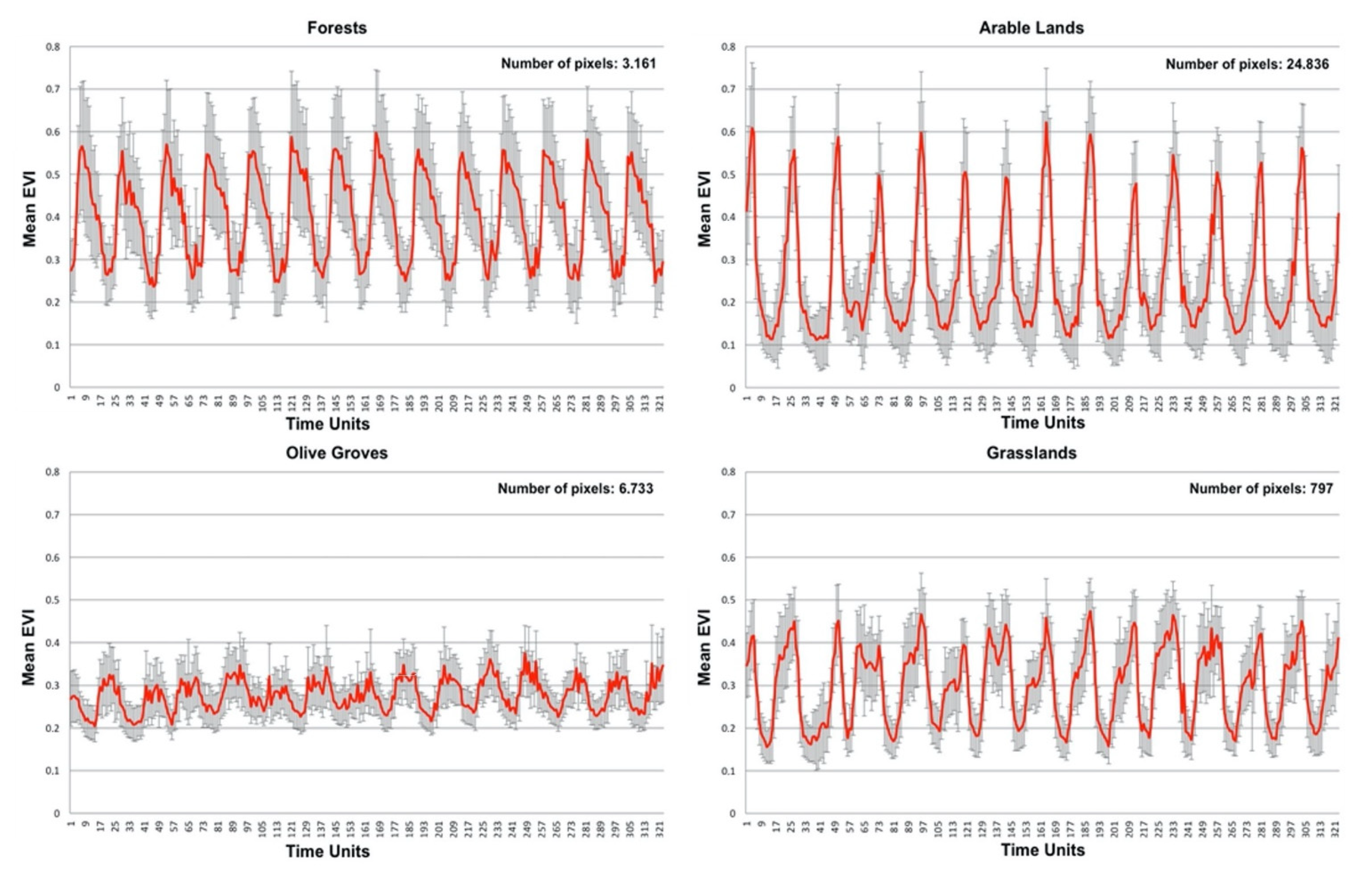
Mean EVI time series of the Apulia region provide a picture of land cover types fluctuating around some trends (increasing or decreasing) or stable average, but with clear differences in the regularities of periodicities and amplitudes of the processes (Figure 3). Broadleaf Forests present the highest average EVI with clear periodicities, with a maximum EVI in late spring (May) and a minimum in winter (February). In contrast, Olive Groves show irregular periodicities with lower amplitude, with a maximum EVI in winter (January) and a minimum in summer (July). Arable Lands show periodicities that clearly reflect the cycle of agricultural practices such as sowing, irrigation and growing, and harvesting, with a maximum EVI in spring (April) and a minimum in July. Grasslands, including semi-arid grasslands, garigues, steppes and pastures, show irregular periodicities with higher amplitude than Olive Groves but with a similar average EVI, with reduced photosynthetic activity in the summer.
Cross-correlations of the EVI with temperature and precipitation demonstrate that most of the time series are consistent with a climatic forcing and variability (Figure 4). However, cross-correlations for Forests are antithetical to those of other types of land cover as forests’ greater self-organization makes them almost independent of precipitation events. In contrast, there is an evident direct correlation between the EVI of Forests and temperature. For Arable Lands, the cross-correlations with both precipitation and temperature are negative, highlighting that water availability is not dependent on precipitation events, but on groundwater for irrigation. The cross-correlation between precipitation and Olive Groves behaves similarly to Grasslands, which shows a strong dependence on precipitation events. However, Olive Groves are negatively related to temperature, with the highest EVI in winter.
3.2. RP and RQA Analysis
The visual appearance of recurrence plots (Figure 5) provides many hints about the functional dynamics of land covers and their stability and predictability.
Distances between diagonal lines, i.e., the period of the oscillation appear rather similar among the types of land cover. Higher predictability, determinism, recurrence rates and Lmax shown by Forests and Arable Lands mean that the dynamics of both land cover types are rather persistent and predictable, with strong periodic components (Table 2). Relatively high laminarity means intermittency in the EVI of Forests whenever some states do not change or change slowly.
Forests and Arable Lands are more stable and resilient than Olive Groves and Grasslands, with effects on the provision of landscape services associated with the first two land cover classes. Forests and Arable Lands are rather quasi-periodic, but with determinism (DET) greater for Forests than for Arable Lands (Table 2). For Arable Lands, some states do not change or change slowly as an effect of human-managed balancing feedback loops at work (irrigation versus drought, soil fertilization versus soil impoverishment, etc.).
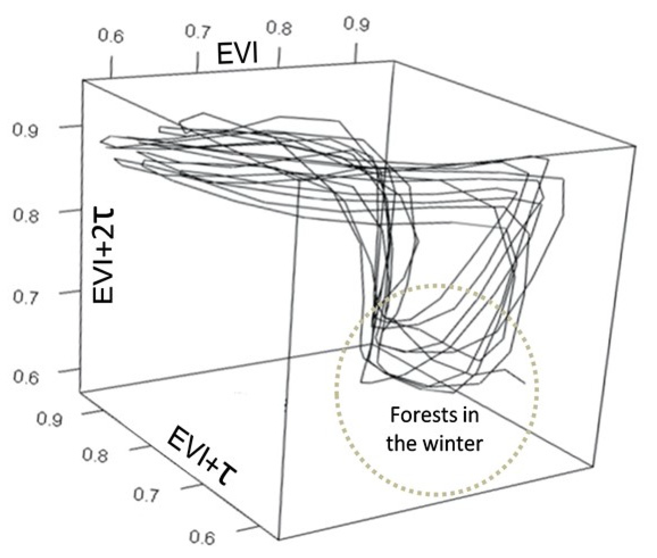
The three-dimensional reconstruction of the EVI time delays in the phase space for Forests shows that the trajectories remained approximately in the same phase space in fourteen years, exhibiting the greatest stability and predictability with a minimum EVI in winter (Figure 6). Such a three-dimensional reconstruction supports the existence of much less temporal variation in CO2 fluxes than commonly assumed for trees subjected to periodic photosynthetic down-regulation [62].
3.3. Maps of Recurrence Variables and Hot Spots Undergoing Degradation and Desertification (LDD)
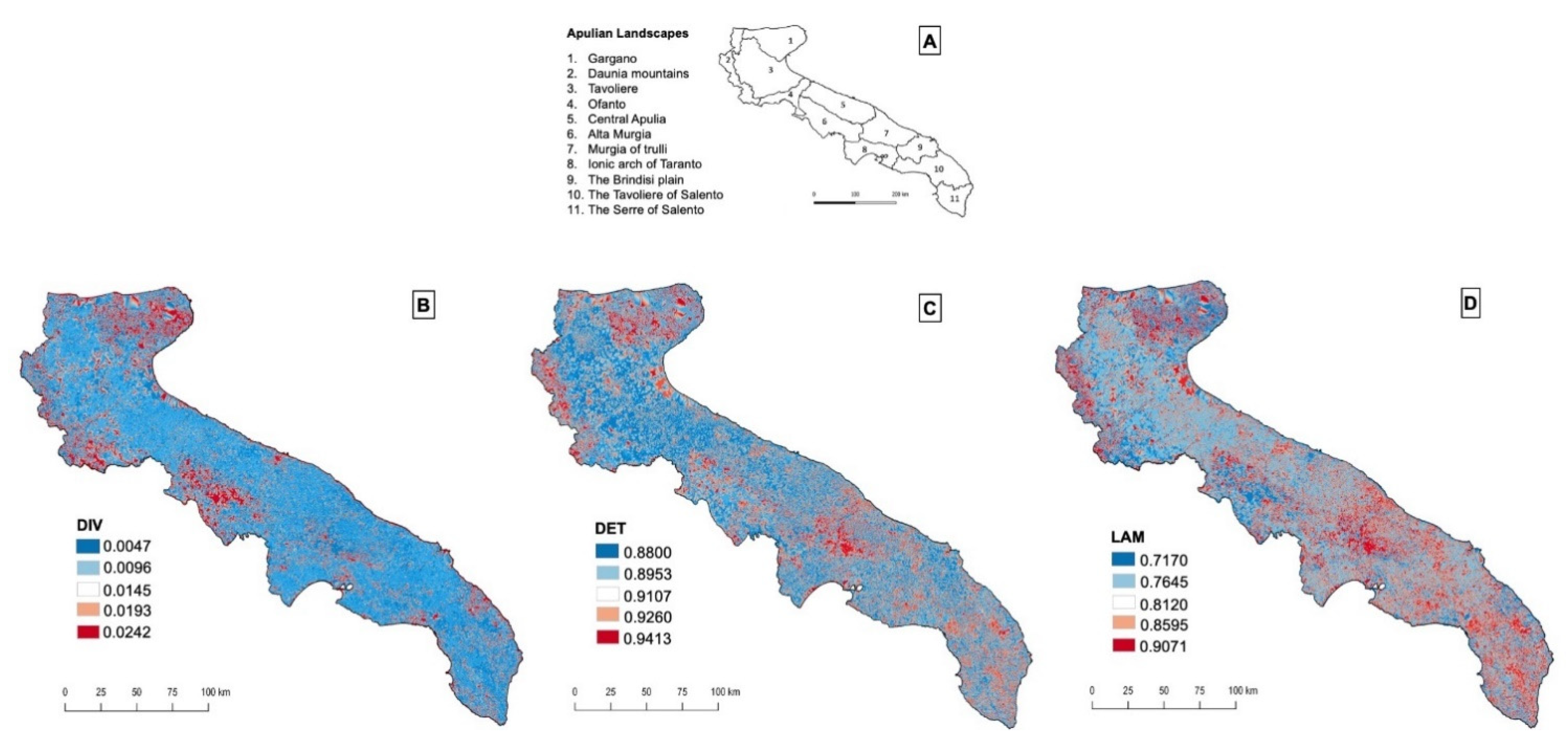
The most significant recurrence variables related to predictability (Determinism, DET; Laminarity, LAM) and chaoticity (Divergence, DIV) for Apulia were mapped (Figure 7B–D) for the four most representative land cover types (Forests, Olive Groves, Arable Lands, Grasslands) together with recurrence estimates of other Corine land covers (Figure 1) [63] derived from randomly selected MODIS pixels.
The maps clearly show regions characterized by a greater recurrence (high predictability, DET, LAM, Figure 7C,D) mainly linked to the National Park of Gargano (1 in Figure 7A), Murgia of Trulli (7 in Figure 7A), the northern Daunia mountains (2 in Figure 7A) and extensive olive groves (9,10,11 in Figure 7A).
Conversely, evident and coherent space clusters, less predictable and with more chaoticity (higher divergence, DIV) (Figure 7B), are clearly identifiable in central Alta Murgia (6 in Figure 7A), in the Gargano plateau (1 in Figure 7A) and in the southern Daunia mountains (2 in Figure 7A). In all these areas, the Grasslands class, including semi-arid grasslands, garrigue, steppes and permanent pastures, has its highest concentration. These three areas correspond exactly to already known regional hot spots [19,29,31,64,65] with land desertification in progress.
More specifically, the central Alta Murgia area (6 in Figure 7A) is a limestone plateau primarily used as pastures with widespread surface features: karst and layers of outcropping rock with discontinuous and thin soils where xeric grasslands cover almost 24% of the total area. In this area, the Alta Murgia National Park is present (67,739 ha), which covers most of the territory and represents one of the most important conservation areas in Europe for the presence of habitats listed in the 92/43/EEC Habitat Directive with the highest priority for conservation, such as semi-natural dry grasslands and scrubland facies on calcareous substrates (Festuco-Brometalia), pseudo-steppe with grasses and annuals of the Thero-Brachypodietea* and eastern sub-Mediteranean dry grasslands (Scorzoneratalia villosae) [66].
In this area, the greatest decrease (−26%) in the extent of xeric grasslands from 1990 to 2018 is already known, and it has been mainly due to their conversion to Arable Lands [67] by extensive interventions of mechanical “stone crushing” (up to pulverization) of the soil-calcareous rock with the emergence of less productive shrublands [67]. This practice is banned nowadays.
As a result, in reclaimed arable lands, crops (mainly wheat) cover the thin soil for few months a year, and this increases the exposure to extreme weather events. The soil structural characteristics worsen as the percentage of organic matter decreases and the inert fine particles increase. Therefore, during heavy rains, even with moderate slopes, part of these low-quality soils can slide along the slopes [19]. Therefore, some pixels belonging to Arable Lands also contributed to the chaoticity in the area.
Another relevant cluster of high divergence with more chaotic greenness behavior is represented by the Gargano karst plateau (1 in Figure 7A), which occupies, from west to east, the central nucleus of the Gargano National Park. It is characterized by rangelands with bald and stony ridges alternating with woods. It is a karst environment, characterized by fields of sinkholes and tombs, with the alternation of semi-arid grasslands and pastures with trees, arable land and wooded areas. Here, the frequency of fires [21,68] has historically promoted the adaptation of evergreen trees such as Pinus halepensis and grasses such as Hyparrhenia hirta and Brachypodium ramosum, which can recover after fire disturbances [21]. The severity of the fire event influences the surface hydrological response and the consequent loss of soil. In the years following the fire, soil loss could be quite high and soil degradation processes much greater than before the event [19].
Finally, the third spatial cluster of high divergence is the South Daunia mountains (2 in Figure 7A), mainly associated with semi-arid grasslands, garrigue, steppes and permanent pastures, but also with land degradation for slope instability and subsequent landslides during seasonal rainfalls because of land use conversion and land abandonment [69,70]. Most of the unfavorable biophysical factors affecting Alta Murgia also occur substantially for southern Daunia.
4. Discussion
There are several approaches proposed for land degradation and desertification (LDD) analysis. One of the most popular spatially evaluates variables and indicators without considering their dynamics to map specific LDD issues through the recombination of thematic layers (e.g., [19,31,34,71]). However, all these studies are static and limited to the generation of desertification risk maps.
On the other hand, remote sensing-based analyses of vegetation cover decline rely on a wide range of change detection methods [72]. One approach is based on image classification when multitemporal Land Use Land Cover (LULC) maps are compared to identify changes (e.g., [73]). Such classification-based analyses, however, fail to evaluate the temporal evolution of LDD processes and can lead to high mapping inaccuracies due to error propagation between LULC classification results. Trend analyses of multi-year satellite images allow the capture of gradual LDD processes [74], but they are not independent from constraining assumptions like linearity. Trend analyses were routinely employed for LDD assessment using coarse- and multi-temporal imagery [75].
The present non-linear approach, based on the integration EVI-RQA, represents a clear novelty in the approaches for LDD assessment. It is a multi-temporal satellite analysis where non-linear time series analysis techniques are applied to extract information from time series of EVI pixels useful to analyze their complex behavior. It can also be useful in making the MEA definition of LDD operational, as poor and erodible soils, erratic precipitation (mainly during the winter), high summer temperatures with frequent drought events, land use conversion, extensive deforestation with frequent wildfires, and land abandonment can significantly reduce the ability of vegetation cover to provide, regulate and support landscape services. All these factors reverberate on the greater chaotic behavior of the EVI time series over time, mainly for the general Grasslands class (divergence, DIV; Table 2, Figure 7B). Therefore, greater chaoticity (less resilience) of the EVI over time can indicate LDD.
The results have shown that Forests and Arable Lands are more stable and resilient than Olive Groves and Grasslands, with effects on the provision of landscape services associated with the first two land cover classes. Forests and Arable Lands are rather quasi-periodic, but with determinism (DET) greater for Forests than for Arable Lands (Table 2). Specifically, for Arable Lands, some states do not change or change slowly, as highlighted by relatively high DET just with some intermittency, so that some states change slowly because of agricultural practices characterized by some periodic components. However, under human control, there are stress-responsive life-history strategies as for wheat (Triticum turgidum ssp. durum), whose cultivars exhibit traits adapted to both drought and heat [76].
The recurrent behavior of EVI trajectories as a proxy of ANPP indicates that services provided by Forests and Arable Lands are expected to continue with current balancing feedback loops at work. Some Mediterranean forests show, according to Garbulsky and colleagues [77], a low temporal variability in their EVI, being the coefficient of variation less than 10%. This is confirmed by the high DET, REC, Lmax and LAM values and the relatively very low DIV values for Forests (Table 2). Moreover, Mediterranean forests exhibit the highest determinism of the EVI (A N P P) (Table 2), suggesting a strong self-organizing component resistant to the noise structure of the hydroclimatic forcing. These results are like those for European temperate forests, which are largely able to maintain relatively constant physiological settings and water retention even during severe drought and heat events [78]. Apulian evergreen forests are apparently in balance with the Mediterranean climate. This because their sclerophyllous oaks (Quercus ilex, Q. calliprinos and Q. coccifera) and Pinus halepensis represent the woody climax at the end of successional dynamics that can be achieved where biophysical factors remain favorable [79,80].
Permanent Olive Groves have seen their concentration and intensification increase like in other Mediterranean countries [81]. Olive Grove time series show shorter and more interrupted diagonals (Figure 5); therefore, this land cover class is less periodic and less persistent than the century-old olive groves, which are more sparsely distributed probably because the management is based on traditional ecological knowledge and it is considered a best sustainable practice with benefits for the provision of landscape services. Hence, the recurrence rate of Olive Groves is lower than Forests and Arable Lands (Table 2). Their behavior appears more like Grasslands as satellite images also capture the grassy vegetation of the undergrowth. Olive Groves are moderately irrigated, and those laminarity states mainly occur because of balancing physiological feedback controls that determine under summer water stress less stomatal conductance and lower photosynthetic rates to avoid drought-induced hydraulic failure [82], and hence lower values of EVI. As a result of the adaptation of single olive trees to drought, traditional olive groves present an opposite periodicity with a maximum EVI in winter, and this can explain the lower amplitude of their periodic component.
In addition, the slight increasing trend of EVI time series of Olive Groves (Figure 3) may reflect the merging and enlarging of olive groves with the transition from ancient and traditionally managed farms, consisting of widely spaced century-old olive trees surrounded by a grassland matrix used for grazing animals, to modern and mechanical managed farms where olive trees are tightly packed with fewer grasses and more shrubs [81]. This replacement can be interpreted in terms of biodiversity loss as well as a decrease in the landscape services provided by century-old olive groves.
Natural Grasslands are also known for physiological balancing feedback loops inhibiting or reducing photosynthetic activity to adjust their responses to drought. Despite these adaptations, divergence is greatest for Grasslands, implying a more chaotic (less stable) signal (Table 2). This occurs because the structural dynamics and eco-physiological activity of xeric grasslands are mainly driven by discrete inputs or “pulses” of increasing seasonal precipitation [83] (Figure 4). Furthermore, there is an added spatial chaotic effect due to the unceasing conversion of natural Grasslands to Arable Lands through stone removal and crushing. From Table 2, it is evident that the divergence of Grasslands is six times greater than that of Forests. Finally, predictability decreases significantly from closed canopies to open drylands, i.e., from Forests to Grasslands, while chaoticity increases (Table 2). If degradation and desertification worsen due to climate change and/or water shortages, xeric grasslands are likely the first system to degrade, and, therefore, this land cover type should be monitored as it represents the weakest state through which desertification can occur and spread.
5. Conclusions
The spatialization of recurrence variables from non-linear RP-RQA represents a clear novelty among the integrated approaches used for the monitoring and assessment of soil degradation and desertification (LDD). Its strength lies in the applicability to relatively short time-series, its complete independence from binding hypotheses and signal transformations, and in the provision of resilience-related recurrence variables that can be applied spatially to inform planning and management choices. This is fundamental to identify new sustainable landscape planning, intervention, and management choices, based on functional stability and predictability patterns. The approach could be used alone or alongside the traditional ones, based mainly on static structural knowledge.
The approach presented here measures persistent recurrence and chaoticity over time, and it appears to provide an efficient method to quantify and spatialize functional dynamic stability and predictability in dryland SELs, as well as to gauge the phase and function instabilities, which are otherwise undetectable. The mapping of the recurrence variables summarizes the (ir)regularity of the different land cover functional dynamics, providing a powerful insight to discriminate between areas with different stability/predictability in the landscape.
The effectiveness of this approach is validated by its ability to confirm already known hot spots with ongoing land desertification processes. However, its potentiality is to identify new areas of interest where to focus new more specific in situ investigations. In this perspective, the divergence (DIV) variable, represented by the chaoticity (lower resilience) of the EVI time series over time, could be used as a novel index, making the MEA definition of LDD operational.
The challenging goal of achieving the neutrality of soil degradation (LDN) by 2030 set by the United Nation Sustainable Development Goal (SDG) requires new conceptual strategies for analyzing and designing landscape sustainability models. In the case of drylands, they could include the strategic conservation of forests and xeric grasslands as well as the strategic planning of landscape conversion to reduce the intensity of water and soil stress.
Finally, it is well known that the future is not likely to be a simple extrapolation of the recent past because unexpected events can suddenly happen, as well as the recent exacerbated effects of climate change. However, having the knowledge of recent recurrence dynamics of vegetation cover from non-linear RP-RQA and of the spatial distribution of recurrence variables can assist in management and policies and foster the stability and short-term predictability (resilience) of dryland dynamics, guaranteeing the provision of landscape services.
Author Contributions
Conceptualization, G.Z., I.P., K.B.J., B.-L.L.; software, D.V.; validation, D.V., I.P., C.M.; formal analysis, I.P., D.V., C.M.; investigation, D.V., I.P.; resources, D.V., I.P.; data curation, D.V., G.Z., C.M.; writing—original draft preparation, G.Z., C.M., K.B.J., I.P.; writing—review and editing, K.B.J., C.M., I.P., D.V.; visualization, D.V.; supervision, I.P., G.Z. All authors have read and agreed to the published version of the manuscript.
Funding
This research received no external funding.
Institutional Review Board Statement
Not applicable.
Informed Consent Statement
Not applicable.
Data Availability Statement
Data available on request.
Conflicts of Interest
The authors declare no conflict of interest.
References
- Levin, S.A. Ecosystems and the biosphere as complex adaptive systems. Ecosystems 1998, 1, 431–436. [Google Scholar] [CrossRef]
- Berkes, F.; Colding, J.; Folke, E. Navigating Social–Ecological Systems: Building Resilience for Complexity and Change; Cambridge University Press: Cambridge, UK, 2003. [Google Scholar]
- Zaccarelli, N.; Petrosillo, I.; Zurlini, G.; Riitters, K.H. Source/sink patterns of disturbance and cross-scale mismatches in a panarchy of social-ecological landscapes. Ecol. Soc. 2008, 13, 26. [Google Scholar] [CrossRef]
- Scheffer, M.; Carpenter, S.R. Catastrophic regime shifts in ecosystems: Linking theory to observation. Trends Ecol. Evol. 2003, 18, 648–656. [Google Scholar] [CrossRef]
- Reynolds, J.F.; Smith, D.M.S.; Lambin, E.F.; Turner, B.L., II; Mortimore, M.; Batterbury, S.P.J.; Downing, T.E.; Dowlatabadi, H.; Fernández, R.J.; Herrick, J.E.; et al. Global Desertification: Building a Science for Dryland Development. Science 2007, 316, 847–851. [Google Scholar] [CrossRef] [PubMed] [Green Version]
- Reid, W.V.; Mooney, H.A.; Cropper, A.; Capistrano, D.; Carpenter, S.R.; Chopra, K.; Dasgupta, P.; Dietz, T.; Duraiappah, A.K.; Hassan, R.; et al. Ecosystems and Human Well-Being: Synthesis; Island Press: Washington, DC, USA, 2005. [Google Scholar]
- Termorshuizen, J.W.; Opdam, P. Landscape services as a bridge between landscape ecology and sustainable development. Landsc. Ecol. 2009, 24, 1037–1052. [Google Scholar] [CrossRef]
- Costanza, R.; Fisher, B.; Mulder, K.; Liu, S.; Christopher, T. Biodiversity and ecosystem services: A multi-scale empirical study of the relationship between species richness and net primary production. Ecol. Econ. 2007, 61, 478–491. [Google Scholar] [CrossRef]
- Odum, H. Environment, Power, and Society; John Wiley & Sons: New York, NY, USA, 1971. [Google Scholar]
- Gaston, K.J. Global patterns in biodiversity. Nature 2000, 405, 220–227. [Google Scholar] [CrossRef]
- Vogt, J.V.; Safriel, U.; von Maltitz, G.; Sokona, Y.; Zougmore, R.; Bastin, G.; Hill, J. Monitoring and assessment of land degradation and desertification: Towards new conceptual and integrated approaches. Land Degrad. Dev. 2011, 22, 150–165. [Google Scholar] [CrossRef]
- Dubovyk, O. The role of Remote Sensing in land degradation assessments: Opportunities and challenges. Eur. J. Remote Sens. 2017, 50, 601–613. [Google Scholar] [CrossRef]
- Zhang, G.; Biradar, C.M.; Xiao, X.; Dong, J.; Zhou, Y.; Qin, Y.; Zhang, Y.; Liu, F.; Ding, M.; Thomas, R.J. Exacerbated grassland degradation and desertification in Central Asia during 2000–2014. Ecol. Appl. 2018, 28, 442–456. [Google Scholar] [CrossRef] [PubMed] [Green Version]
- Marwan, N.; Romano, M.C.; Thiel, M.; Kurths, J. Recurrence plots for the analysis of complex systems. Phys. Rep. 2007, 438, 237–329. [Google Scholar] [CrossRef]
- Peterson, G.D. Estimating Resilience Across Landscapes. Conserv. Ecol. 2002, 6, 17. [Google Scholar] [CrossRef] [Green Version]
- Xiao, X.; Hollinger, D.; Aber, J.; Goltz, M.; Davidson, E.A.; Zhang, Q.; Moore, B. Satellite-based modeling of gross primary production in an evergreen needleleaf forest. Remote Sens. Environ. 2004, 89, 519–534. [Google Scholar] [CrossRef]
- Petrosillo, I.; Semeraro, T.; Zaccarelli, N.; Aretano, R.; Zurlini, G. The possible combined effects of land-use changes and climate conditions on the spatial-temporal patterns of primary production in a natural protected area. Ecol. Indic. 2013, 29, 25. [Google Scholar] [CrossRef]
- Zurlini, G.; Li, B.-L.; Zaccarelli, N.; Petrosillo, I. Spectral entropy, ecological resilience, and adaptive capacity for understanding, evaluating, and managing ecosystem stability and change. Glob. Chang. Biol. 2015, 21, 1377–1378. [Google Scholar] [CrossRef] [PubMed]
- Ladisa, G.; Todorovic, M.; Liuzzi, G.T. A GIS-based approach for desertification risk assessment in Apulia region, SE Italy. Phys. Chem. Earth Parts A B C 2012, 49, 103–113. [Google Scholar] [CrossRef]
- Nieto-Romero, M.; Oteros-Rozas, E.; González, J.A.; Martín-López, B. Exploring the knowledge landscape of ecosystem services assessments in Mediterranean agroecosystems: Insights for future research. Environ. Sci. Policy 2014, 37, 121–133. [Google Scholar] [CrossRef]
- Zurlini, G.; Marwan, N.; Semeraro, T.; Jones, K.B.; Aretano, R.; Pasimeni, M.R.; Valente, D.; Mulder, C.; Petrosillo, I. Investigating landscape phase transitions in Mediterranean rangelands by recurrence analysis. Landsc. Ecol. 2018, 33, 1617–1631. [Google Scholar] [CrossRef]
- Tarrasón, D.; Ravera, F.; Reed, M.S.; Dougill, A.J.; Gonzalez, L. Land degradation assessment through an ecosystem services lens: Integrating knowledge and methods in pastoral semi-arid systems. J. Arid Environ. 2016, 124, 205–213. [Google Scholar] [CrossRef]
- Smith, W.K.; Dannenberg, M.P.; Yan, D.; Herrmann, S.; Barnes, M.L.; Barron-Gafford, G.A.; Biederman, J.A.; Ferrenberg, S.; Fox, A.M.; Hudson, A.; et al. Remote sensing of dryland ecosystem structure and function: Progress, challenges, and opportunities. Remote Sens. Environ. 2019, 233, 111401. [Google Scholar] [CrossRef]
- Pueyo, Y.; Alados, C.L. Effects of fragmentation, abiotic factors and land use on vegetation recovery in a semi-arid Mediterranean area. Basic Appl. Ecol. 2007, 8, 158–170. [Google Scholar] [CrossRef]
- Kapur, B.; Pasquale, S.; Tekin, S.; Todorovic, M.; Sezen, S.M.; Özfidaner, M.; Gümü, Z. Prediction of climatic change for the next 100 years in Southern Italy. Sci. Res. Essays 2010, 5, 1470. [Google Scholar]
- Caroli, I.; Caldara, M. Vegetation history of Lago Battaglia (eastern Gargano coast, Apulia, Italy) during the middle-late Holocene. Veg. Hist. Archaeobotany 2007, 16, 317–327. [Google Scholar] [CrossRef]
- Di Rita, F.; Simone, O.; Caldara, M.; Gehrels, W.R.; Magri, D. Holocene environmental changes in the coastal Tavoliere Plain (Apulia, southern Italy): A multiproxy approach. Palaeogeogr. Palaeoclimatol. Palaeoecol. 2011, 310, 139–151. [Google Scholar] [CrossRef]
- Perini, L.; Ceccarelli, T.; Zitti, M.; Salvati, L. Insight desertification process: Bio-physical and socio-economic drivers in Italy. Ital. J. Agrometeorol. 2009, 3, 45–55. [Google Scholar]
- Benassi, F.; Cividino, S.; Cudlin, P.; Alhuseen, A.; Lamonica, G.R.; Salvati, L. Population trends and desertification risk in a Mediterranean region, 1861–2017. Land Use Policy 2020, 95, 104626. [Google Scholar] [CrossRef]
- Giorgi, F.; Lionello, P. Climate change projections for the Mediterranean region. Glob. Planet. Chang. 2008, 63, 90–104. [Google Scholar] [CrossRef]
- Salvati, L.; Mavrakis, A.; Colantoni, A.; Mancino, G.; Ferrara, A. Complex Adaptive Systems, soil degradation and land sensitivity to desertification: A multivariate assessment of Italian agro-forest landscape. Sci. Total Environ. 2015, 521–522, 235–245. [Google Scholar] [CrossRef]
- Metzger, M.J.; Rounsevell, M.D.A.; Acosta-Michlik, L.; Leemans, R.; Schröter, D. The vulnerability of ecosystem services to land use change. Agric. Ecosyst. Environ. 2006, 114, 69–85. [Google Scholar] [CrossRef]
- Petrosillo, I.; Zaccarelli, N.; Zurlini, G. Multi-scale vulnerability of natural capital in a panarchy of social-ecological landscapes. Ecol. Complex. 2010, 7, 359–367. [Google Scholar] [CrossRef]
- Salvati, L.; Bajocco, S.; Ceccarelli, T.; Zitti, M.; Perini, L. Towards a process-based evaluation of land vulnerability to soil degradation in Italy. Ecol. Indic. 2011, 11, 1216–1227. [Google Scholar] [CrossRef]
- Briassoulis, H. Mediterranean Desertification—Framing The Policy Context. EU DG for Research: Sustainable Development, Global Change and Ecosystem; Publications Office of the EU: Luxembourg, 2003. [Google Scholar]
- Acosta-Michlik, L.A.; Kumar, K.S.K.; Klein, R.J.T.; Campe, S. Application of fuzzy models to assess susceptibility to droughts from a socio-economic perspective. Reg. Environ. Chang. 2008, 8, 151–160. [Google Scholar] [CrossRef]
- Potter, C.; Tan, P.N.; Steinbach, M.; Klooster, S.; Kumar, V.; Myneni, R.; Genovese, V. Major disturbance events in terrestrial ecosystems detected using global satellite data sets. Glob. Chang. Biol. 2003, 9, 1005–1021. [Google Scholar] [CrossRef] [Green Version]
- Fu, X.; Tang, C.; Zhang, X.; Fu, J.; Jiang, D. An improved indicator of simulated grassland production based on MODIS NDVI and GPP data: A case study in the Sichuan province, China. Ecol. Indic. 2014, 40, 102–108. [Google Scholar] [CrossRef]
- Yan, D.; Scott, R.L.; Moore, D.J.P.; Biederman, J.A.; Smith, W.K. Understanding the relationship between vegetation greenness and productivity across dryland ecosystems through the integration of PhenoCam, satellite, and eddy covariance data. Remote Sens. Environ. 2019, 223, 50–62. [Google Scholar] [CrossRef]
- Huete, A.; Didan, K.; Miura, T.; Rodriguez, E.P.; Gao, X.; Ferreira, L.G. Overview of the radiometric and biophysical performance of the MODIS vegetation indices. Remote Sens. Environ. 2002, 83, 195–213. [Google Scholar] [CrossRef]
- Potter, C.; Klooster, S.; Genovese, V. Net primary production of terrestrial ecosystems from 2000 to 2009. Clim. Chang. 2012, 115, 365–378. [Google Scholar] [CrossRef] [Green Version]
- Boegh, E.; Soegaard, H.; Broge, N.; Hasager, C.B.; Jensen, N.O.; Schelde, K.; Thomsen, A. Airborne multispectral data for quantifying leaf area index, nitrogen concentration, and photosynthetic efficiency in agriculture. Remote Sens. Environ. 2002, 81, 179–193. [Google Scholar] [CrossRef]
- Xiao, X.; Braswell, B.; Zhang, Q.; Boles, S.; Frolking, S.; Moore, B. Sensitivity of vegetation indices to atmospheric aerosols: Continental-scale observations in Northern Asia. Remote Sens. Environ. 2003, 84, 385–392. [Google Scholar] [CrossRef]
- Wallace, C.; Thomas, K. An Annual Plant Growth Proxy in the Mojave Desert Using MODIS-EVI Data. Sensors 2008, 8, 7792–7808. [Google Scholar] [CrossRef] [Green Version]
- Zaccarelli, N.; Li, B.-L.; Petrosillo, I.; Zurlini, G. Order and disorder in ecological time-series: Introducing normalized spectral entropy. Ecol. Indic. 2013, 28, 22–30. [Google Scholar] [CrossRef]
- Li, B.-L. Why is the holistic approach becoming so important in landscape ecology? Landsc. Urban Plan. 2000, 50, 27–41. [Google Scholar] [CrossRef]
- Strang, G. Wavelets. Am. Sci. 1994, 83, 250–255. [Google Scholar]
- Marwan, N. A historical review of recurrence plots. Eur. Phys. J. Spec. Top. 2008, 164, 3–12. [Google Scholar] [CrossRef] [Green Version]
- Soudani, K.; Maire, G.; Dufrêne, E.; François, C.; Delpierre, N.; Ulrich, E.; Cecchini, S. Evaluation of the onset of green-up in temperate deciduous broadleaf forests derived from Moderate Resolution Imaging Spectroradiometer (MODIS) data. Remote Sens. Environ. 2008, 112, 2643–2655. [Google Scholar] [CrossRef]
- Vretenar, D.; Paar, N.; Ring, P.; Lalazissis, G.A. Nonlinear dynamics of giant resonances in atomic nuclei. Phys. Rev. E 1999, 60, 308–319. [Google Scholar] [CrossRef] [Green Version]
- Rustici, M.; Caravati, C.; Petretto, E.; Branca, M.; Marchettini, N. Transition Scenarios during the Evolution of the Belousov−Zhabotinsky Reaction in an Unstirred Batch Reactor. J. Phys. Chem. A 1999, 103, 6564–6570. [Google Scholar] [CrossRef]
- Marwan, N.; Wessel, N.; Meyerfeldt, U.; Schirdewan, A.; Kurths, J. Recurrence-plot-based measures of complexity and their application to heart-rate-variability data. Phys. Rev. E 2002, 66, 026702. [Google Scholar] [CrossRef] [Green Version]
- Belaire-Franch, J.; Contreras, D.; Tordera-Lledó, L. Assessing nonlinear structures in real exchange rates using recurrence plot strategies. Phys. D Nonlinear Phenom. 2002, 171, 249–264. [Google Scholar] [CrossRef] [Green Version]
- Marwan, N.; Kurths, J.; Foerster, S. Analysing spatially extended high-dimensional dynamics by recurrence plots. Phys. Lett. A 2015, 379, 894–900. [Google Scholar] [CrossRef] [Green Version]
- Li, S.; Zhao, Z.; Wang, Y.; Wang, Y. Identifying spatial patterns of synchronization between NDVI and climatic determinants using joint recurrence plots. Environ. Earth Sci. 2011, 64, 851–859. [Google Scholar] [CrossRef]
- Gallopín, G.C. Linkages between vulnerability, resilience, and adaptive capacity. Glob. Environ. Chang. 2006, 16, 293–303. [Google Scholar] [CrossRef]
- Tonkin, J.D.; Bogan, M.T.; Bonada, N.; Rios-Touma, B.; Lytle, D.A. Seasonality and predictability shape temporal species diversity. Ecology 2017, 98, 1201–1216. [Google Scholar] [CrossRef] [Green Version]
- Colwell, R.K. Predictability, Constancy, and Contingency of Periodic Phenomena. Ecology 1974, 55, 1148–1153. [Google Scholar] [CrossRef]
- Walker, B.; Holling, C.S.; Carpenter, S.R.; Kinzig, A. Resilience, Adaptability and Transformability in Social—Ecological Systems. Ecol. Soc. 2004, 9, 5. [Google Scholar] [CrossRef]
- Carpenter, S.; Walker, B.; Anderies, J.M.; Abel, N. From Metaphor to Measurement: Resilience of What to What? Ecosystems 2001, 4, 765–781. [Google Scholar] [CrossRef]
- Wuertz, D.; Setz, T.; Chalabi, Y. R Package ‘fNonlinear’. Available online: http://cran.r-project.org/web/packages/fNonlinear/index.html (accessed on 25 June 2020).
- Garbulsky, M.F.; Peñuelas, J.; Gamon, J.; Inoue, Y.; Filella, I. The photochemical reflectance index (PRI) and the remote sensing of leaf, canopy and ecosystem radiation use efficienciesA review and meta-analysis. Remote Sens. Environ. 2011, 115, 281–297. [Google Scholar] [CrossRef]
- Heymann, Y.; Steenmans, C.; Croissille, G.; Bossard, M. Corine Land Cover. Technical Guide; Commission of the European Communities: Luxembourg, 1994. [Google Scholar]
- Santarsiero, V.; Nolè, G.; Lanorte, A.; Tucci, B.; Saganeiti, L.; Pilogallo, A.; Scorza, F.; Murgante, B. Assessment of Post Fire Soil Erosion with ESA Sentinel-2 Data and RUSLE Method in Apulia Region. (Southern Italy); Springer: Cham, Germany, 2020; pp. 590–603. [Google Scholar]
- Salvati, L.; Zitti, M.; Perini, L. Fifty Years on: Long-term Patterns of Land Sensitivity to Desertification in Italy. Land Degrad. Dev. 2016, 27, 97–107. [Google Scholar] [CrossRef]
- Fracchiolla, M.; Terzi, M.; D’Amico, F.S.; Tedone, L.; Cazzato, E. Conservation and pastoral value of former arable lands in the agro-pastoral system of the Alta Murgia National Park (Southern Italy). Ital. J. Agron. 2017, 11. [Google Scholar] [CrossRef] [Green Version]
- Tarantino, C.; Adamo, M.; Blonda, P. Long-Term Change Monitoring of Natural Grasslands Ecosystem in Support Of SDG 15.3.1. In Proceedings of the EGU General Assembly Conference Abstracts, Vienna, Australia , 3–8 May 2020. [Google Scholar]
- Zurlini, G.; Petrosillo, I.; Jones, K.B.; Zaccarelli, N. Highlighting order and disorder in social-ecological landscapes to foster adaptive capacity and sustainability. Landsc. Ecol. 2013, 28, 1161–1173. [Google Scholar] [CrossRef]
- Pellicani, R.; Spilotro, G. Evaluating the quality of landslide inventory maps: Comparison between archive and surveyed inventories for the Daunia region (Apulia, Southern Italy). Bull. Eng. Geol. Environ. 2015, 74, 357–367. [Google Scholar] [CrossRef]
- Pisano, L.; Dragone, V.; Vennari, C.; Vessia, G.; Parise, M. The Influence of Slope Instability Processes in Demographic Dynamics of Landslide-Prone Rural Areas. In Landslides and Engineered Slopes. Experience, Theory and Practice; Cascini, L., Aversa, S., Picarelli, L., Scavia, C., Eds.; Associazione Geotecnica Italiana: Rome, Italy, 2016. [Google Scholar]
- Ferrara, A.; Kosmas, C.; Salvati, L.; Padula, A.; Mancino, G.; Nolè, A. Updating the MEDALUS-ESA Framework for Worldwide Land Degradation and Desertification Assessment. Land Degrad. Dev. 2020, 31, 1593–1607. [Google Scholar] [CrossRef]
- Higginbottom, T.; Symeonakis, E. Assessing Land Degradation and Desertification Using Vegetation Index Data: Current Frameworks and Future Directions. Remote Sens. 2014, 6, 9552–9575. [Google Scholar] [CrossRef] [Green Version]
- Yiran, G.A.B.; Kusimi, J.M.; Kufogbe, S.K. A synthesis of remote sensing and local knowledge approaches in land degradation assessment in the Bawku East District, Ghana. Int. J. Appl. Earth Obs. Geoinf. 2012, 14, 204–213. [Google Scholar] [CrossRef]
- Ghazaryan, G.; Dubovyk, O.; Kussul, N.; Menz, G. Towards an Improved Environmental Understanding of Land Surface Dynamics in Ukraine Based on Multi-Source Remote Sensing Time-Series Datasets from 1982 to 2013. Remote Sens. 2016, 8, 617. [Google Scholar] [CrossRef] [Green Version]
- Santos, F.; Dubovyk, O.; Menz, G. Monitoring Forest Dynamics in the Andean Amazon: The Applicability of Breakpoint Detection Methods Using Landsat Time-Series and Genetic Algorithms. Remote Sens. 2017, 9, 68. [Google Scholar] [CrossRef] [Green Version]
- Aprile, A.; Havlickova, L.; Panna, R.; Marè, C.; Borrelli, G.M.; Marone, D.; Perrotta, C.; Rampino, P.; de Bellis, L.; Curn, V.; et al. Different stress responsive strategies to drought and heat in two durum wheat cultivars with contrasting water use efficiency. BMC Genom. 2013, 14, 821. [Google Scholar] [CrossRef] [PubMed] [Green Version]
- Garbulsky, M.F.; Filella, I.; Verger, A.; Peñuelas, J. Photosynthetic light use efficiency from satellite sensors: From global to Mediterranean vegetation. Environ. Exp. Bot. 2014, 103, 3–11. [Google Scholar] [CrossRef]
- Rennenberg, H.; Loreto, F.; Polle, A.; Brilli, F.; Fares, S.; Beniwal, R.S.; Gessler, A. Physiological Responses of Forest Trees to Heat and Drought. Plant Biol. 2006, 8, 556–571. [Google Scholar] [CrossRef]
- Pignatti, S. Flora d’Italia; Edagricole: Bologna, Italy, 1982. [Google Scholar]
- Biondi, E.; Casavecchia, S.; Guerra, V.; Medagli, P.; Beccarisi, L.; Zuccarello, V. A contribution towards the knowledge of semideciduous and evergreen woods of Apulia (southeastern Italy). Fitosociologia 2004, 41, 3–28. [Google Scholar]
- Ortega, M.; Pascual, S.; Elena-Rosselló, R.; Rescia, A.J. Land-use and spatial resilience changes in the Spanish olive socio-ecological landscape. Appl. Geogr. 2020, 117, 102171. [Google Scholar] [CrossRef]
- Angelopoulos, K.; Dichio, B.; Xiloyannis, C. Inhibition of photosynthesis in olive trees (Olea europaea L.) during water stress and rewatering. J. Exp. Bot. 1996, 47, 1093–1100. [Google Scholar] [CrossRef] [Green Version]
- Huxman, T.E.; Cable, J.M.; Ignace, D.D.; Eilts, J.A.; English, N.B.; Weltzin, J.; Williams, D.G. Response of net ecosystem gas exchange to a simulated precipitation pulse in a semi-arid grassland: The role of native versus non-native grasses and soil texture. Oecologia 2004, 141, 295–305. [Google Scholar] [CrossRef] [PubMed]
Figure 1.
The Apulia Region with the main drivers responsible for land degradation and desertification.
Figure 1.
The Apulia Region with the main drivers responsible for land degradation and desertification.

Figure 2.
Recurrence plots of three prototypical systems: (A) uniformly distributed white noise, (B) fully predictable oscillating motion with sine frequency, and (C) irregular and unpredictable chaotic system [14].
Figure 2.
Recurrence plots of three prototypical systems: (A) uniformly distributed white noise, (B) fully predictable oscillating motion with sine frequency, and (C) irregular and unpredictable chaotic system [14].

Figure 3.
Mean Enhanced Vegetation Index (EVI) time trajectories with standard deviations for pixels of the four main land cover classes (Forests, Arable Lands, Olive Groves, and Grasslands) in Apulia region over 14 years, in 16-day time units.
Figure 3.
Mean Enhanced Vegetation Index (EVI) time trajectories with standard deviations for pixels of the four main land cover classes (Forests, Arable Lands, Olive Groves, and Grasslands) in Apulia region over 14 years, in 16-day time units.

Figure 4.
Cross-correlation analysis between the Enhanced Vegetation Index (EVI) and (left) the mean monthly temperature and (right) bimonthly cumulative precipitations for the main land covers. Dotted lines indicate 95% confidence intervals for the correlation coefficient (CCF) at lag zero.
Figure 4.
Cross-correlation analysis between the Enhanced Vegetation Index (EVI) and (left) the mean monthly temperature and (right) bimonthly cumulative precipitations for the main land covers. Dotted lines indicate 95% confidence intervals for the correlation coefficient (CCF) at lag zero.

Figure 5.
Recurrence plots (RPs) for the main land cover classes in the Apulia region based on 14-year Enhanced Vegetation Index (EVI) time series.
Figure 5.
Recurrence plots (RPs) for the main land cover classes in the Apulia region based on 14-year Enhanced Vegetation Index (EVI) time series.
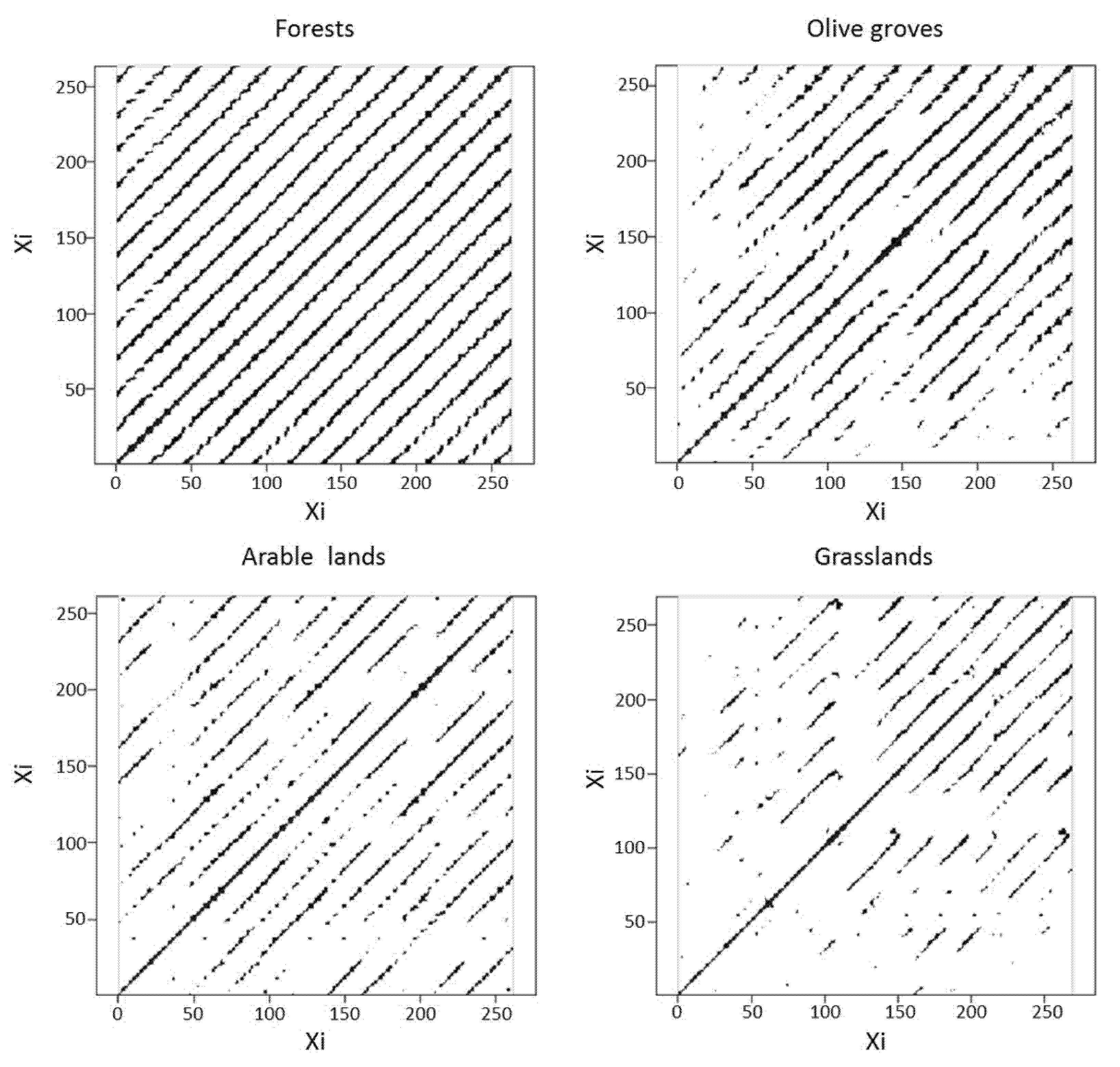
Figure 6.
Three-dimensional reconstruction of the EVI signal in phase space for Forests in Apulia over 14 years using time delays (see the convergence of trajectories in forest phase space during the winter season).
Figure 6.
Three-dimensional reconstruction of the EVI signal in phase space for Forests in Apulia over 14 years using time delays (see the convergence of trajectories in forest phase space during the winter season).

Figure 7.
(A) The Atlas of the eleven main large landscapes characterizing Apulia Region, and the maps of the main recurrence variables (B) Divergence, (C) Determinism, (D) Laminarity.
Figure 7.
(A) The Atlas of the eleven main large landscapes characterizing Apulia Region, and the maps of the main recurrence variables (B) Divergence, (C) Determinism, (D) Laminarity.


Table 1.
Relationships between some recurrence variables (stability metrics) and theoretical descriptors of landscape adaptability.
Table 1.
Relationships between some recurrence variables (stability metrics) and theoretical descriptors of landscape adaptability.
| Recurrence Variable—Stability Metrics | System’s Adaptability Theoretical Descriptors |
|---|---|
| Determinism (DET): the percentage of recurrence points, which form diagonal lines. It gauges the stability and predictability of the dynamical system [14]. | Stability: concentrates on the adaptive capacity of the system to remain within the same domain because of mutually reinforcing structures and processes [56]. |
| Resilience: the probability that a system’s multiple states will persist [15]. | |
| Predictability: the reliability of event recurrence [57]. | |
| Laminarity (LAM): the percentage of recurrence points, which form vertical lines (laminar phases) in the system where some states do not change or change slowly (intermittency) and, hence, the state is trapped for some time [14]. | Constancy: when the state of the system remains the same [58]. |
| Divergence (DIV): the inverse of the length of the longest diagonal line (L max). It gauges the rate at which trajectories diverge and is the hallmark for critical transitions and dynamic chaos [14]. | Precariousness: the proximity or trajectory of an ecosystem state to a threshold that if crossed will result in a regime shift or critical transition [4,59]. Chaoticity: The condition of being chaotic. |
| The longest diagonal line in the plot (L max): the maximum predictability time; the smaller the divergence, the higher the system’s trajectory stability and predictability [14]. | Stability: qualities of a stability domain that resist changes in state or shifts in regime [60]. |
| Resilience: the probability that a system’s multiple states will persist [15]. | |
| Predictability: the reliability of event recurrence [57]. |
Recurrence plots (RPs) and recurrence quantification analysis (RQA) were performed using the R Package “fNonlinear” [61]. Confidence intervals for the recurrence variables were derived from RQAs of 100 random Enhanced Vegetation Index (EVI) time series extracted from each land cover.
Table 2.
Results of RQA for EVI time series for the four land cover classes (Forests, Arable Lands, Olive Groves, Grasslands) in the Apulia region (95% confidence intervals in brackets).
Table 2.
Results of RQA for EVI time series for the four land cover classes (Forests, Arable Lands, Olive Groves, Grasslands) in the Apulia region (95% confidence intervals in brackets).
| Forests | Arable Lands | Olive Groves | Grasslands | |
|---|---|---|---|---|
| DET | 0.948 (0.940–0.956) | 0.930 (0.920–0.938) | 0.880 (0.870–0.890) | 0.891 (0.880–0.901) |
| REC | 0.125 (0.115–0.130) | 0.084 (0.077–0.091) | 0.056 (0.050–0.062) | 0.038 (0.030–0.040) |
| LAM | 0.932 (0.922–0.942) | 0.888 (0.878–0.898) | 0.768 (0.760–0.776) | 0.717 (0.705–0.729) |
| Lmax | 227.03 (218.40–235.60) | 195.10 (187.68–202.50) | 117.20 (112.75–121.65) | 41.3 (39.73–42.87) |
| DIV | 0.0041 (0.0044–0.0040) | 0.0051 (0.0053–0.0049) | 0.0085 (0.0089–0.0080) | 0.0250 (0.0262–0.0242) |
Publisher’s Note: MDPI stays neutral with regard to jurisdictional claims in published maps and institutional affiliations. |
© 2021 by the authors. Licensee MDPI, Basel, Switzerland. This article is an open access article distributed under the terms and conditions of the Creative Commons Attribution (CC BY) license (http://creativecommons.org/licenses/by/4.0/).
Share and Cite
MDPI and ACS Style
Petrosillo, I.; Valente, D.; Mulder, C.; Li, B.-L.; Jones, K.B.; Zurlini, G. The Resilient Recurrent Behavior of Mediterranean Semi-Arid Complex Adaptive Landscapes. Land 2021, 10, 296. https://doi.org/10.3390/land10030296
AMA Style
Petrosillo I, Valente D, Mulder C, Li B-L, Jones KB, Zurlini G. The Resilient Recurrent Behavior of Mediterranean Semi-Arid Complex Adaptive Landscapes. Land. 2021; 10(3):296. https://doi.org/10.3390/land10030296
Chicago/Turabian StylePetrosillo, Irene, Donatella Valente, Christian Mulder, Bai-Lian Li, K. Bruce Jones, and Giovanni Zurlini. 2021. "The Resilient Recurrent Behavior of Mediterranean Semi-Arid Complex Adaptive Landscapes" Land 10, no. 3: 296. https://doi.org/10.3390/land10030296
Note that from the first issue of 2016, this journal uses article numbers instead of page numbers. See further details here.