
Fully Portraying Patch Area Scaling with Resolution: An Analytics and Descriptive Statistics-Combined Approach

1
Faculty of Geosciences and Environmental Engineering, Southwest Jiaotong University, Chengdu 611756, China
2
State-Province Joint Engineering Laboratory of Spatial Information Technology for High-Speed Railway Safety, Southwest Jiaotong University, Chengdu 611756, China
3
National Collaborative Innovation Center for Rail Transport Safety, Southwest Jiaotong University, Chengdu 611756, China
*
Author to whom correspondence should be addressed.
Land 2021, 10(3), 262; https://doi.org/10.3390/land10030262
Submission received: 31 January 2021
/
Revised: 24 February 2021
/
Accepted: 3 March 2021
/
Published: 5 March 2021
(This article belongs to the Special Issue Multiscale Geospatial Approaches for Landscape Ecology)
Abstract
:Scale effects are inherent in spatial analysis. Quantitative knowledge about them is necessary for properly interpreting and scaling analysis results. The objective of this study was to systematically model patch area scaling and the associated uncertainty. A hybrid approach was taken to tackle the difficulty involved. Recognizing that patch’s size and shape play the key role in shaping its scaling behavior, a function model of patch area scaling based on patch morphology was first conceptually formulated. It was then substantiated by sampling and interpolating in the scale-integrated domain of patch morphology, which is characterized by a one-dimensional size index, namely the relative support range (RSR), and a compactness index, namely filling. The area scaling model obtained unveils a simple consistent scaling pattern of all patches and an overall fading range between 0.12 and 3.16 in terms of RSR. The uncertainty model built exhibits a filling-dependent pattern of the variance of patch area, which can be as large as 0.67 (i.e., 67%) in terms of standard deviation. The models were validated by using them to predict patch and class area scaling of the test patches and landscapes. This study demonstrated the basic feasibility of analytically modeling scaling behavior. It also revealed the uncertainty of scale effects is very significant due to the inevitable randomness in rasterization.
1. Introduction
Scale effects refer to the phenomenon that changing the resolution of data used or the extent of study results in varied analysis results [1]. With the increasing use of remote sensing and geographic information system (GIS) for acquiring and analysing spatial data, scale effects have become more and more aware of over decades. They have been encountered in the simple calculation of area or length of geometries [2,3], the straightforward derivation of slope and slope aspect from digital elevation model [4], the modeling of flooding area [5], normalized difference vegetation index (NDVI) [6], and biomass [7] etc. For a relatively recent review, please refer to Sandel [8].
The scale dependence of spatial analysis makes the result of single-scale analysis no longer reliable and needs to be properly interpreted and treated. Efforts have been made to model scale effects for gaining insights [9,10,11,12,13] and for transforming (i.e., scaling) analysis results obtained at certain scales to other scales [14]. Most of the efforts took an empirical approach to modeling the scaling of a metric by fitting a function to the analysis results at multiple scales. Those models were made valid for their respective study area and scale range, but their applicability elsewhere is doubtful due to their lack of generality [15]. Rare research took an analytical approach so as to make the model built widely applicable. That was likely due to the complexity involved as illustrated in Turner et al. [1]. By means of probabilistic modeling of landscape composition and configuration, they analytically predicted for random landscapes the basic characteristics of the scaling behavior of three landscape level metrics, namely diversity, dominance and contagion. But for realistic cases with spatial autocorrelation, the analytical model became too complicated to formulate and be usable. As can be seen, it is difficult to systematically model scale effects. In the empirical approach, the difficulty lies in finding a way to explore the full variation space of scale effects; while in the analytical approach, the model can be too complicated to build and use.
This study aims to systematically and completely model patch area scaling with resolution in aggregation of raster categorical data. Raster categorical data are classified spatial data in raster data structure. They are often the results of classifying remotely sensed images and widely used in spatial analysis. A typical kind of raster categorical data is that of land use and land cover (LULC), which is indispensable for environmental modeling [16,17,18,19,20,21,22]. A patch in raster categorical data is a group of contiguous cells of the same class. The patch is thus the basic semantic unit in raster categorical data and usually corresponds to an entity or a discernible area in real world. A patch’s area is one of its most important properties and is of great concern to environmental modeling [23,24,25,26,27,28,29]. It is common practice in spatial analysis to aggregate raster data to a needed resolution due to limitations of data availability or computing resources [30,31,32]. However, the behavior of patches in aggregation suffers from scale effects. Generally, those small may vanish while larger ones may survive but with its geometry changed to various degree.
For patch area and the related class area of LULC data in particular, earlier empirical work found that scale effects on them did exhibit certain patterns [13] but no widely applicable conclusions were reached at. More focused and systematic efforts were made in recent years. Lechner et al. [33] studied the influence of patch size and length on accurate mapping of small patches and provided valuable quantitative findings. However, the patches used in their study were all simulated and rectangular in shape, while the shape of real-world patches can be arbitrarily complex. Tan et al. [34] noticed the influence of patch morphology on patch scaling and modeled the aggregation effect on patch area by first classifying patches into different shape classes, and then modeling the aggregation effects on each class separately. Their work demonstrated an interesting approach to modeling patch level scale effects. However, there were some limitations in that work, which mainly were: (1) only a small number of sample patches were used for building the model of each class of patches; (2) the classification didn’t seem necessary and introduced extra complication to the modeling; (3) the uncertainty of aggregation was not taken into account.
The objective of this study was to build a quantitative model of patch area scaling that can predict a patch’s area at a given aggregation resolution as well as the uncertainty of the predicted area. The main hypothesis was that patch area scaling can be modeled as a function of patch morphology and the resolution. The models were validated by using them to predict patch and class area scaling of the test patches and landscapes. A hybrid approach was taken in this study to tackling the difficulty involved. Recognizing the critical role of patch morphology (i.e., its size and shape) in characterizing patch’s response to rasterization, a conceptual analytical model was first formulated to capture its dominant influence on the scaling behavior of patch area. Although the functional model was only conceptual and had no concrete mathematical form, it provided a domain in which full exploration of the variation of patch area scaling was made possible, i.e., the morphological domain. The conceptual model was then substantiated by first densely sampling in the domain of patch morphology and then using statistics to obtain a descriptive model. With large enough and well distributed sample population, complete and detailed model of patch area scaling was built, together with the associated uncertainty.
The innovation of this study is that a complete patch area scaling model of raster categorical data is built, which unveils a simple consistent pattern of scaling with RSR for all patches and the filling-dependent fading range of different patches. Besides, it’s the first time that the scaling behavior of a spatial analysis metric is systematically modeled for real world situation.
The rest of the paper is organized as follows. Section 2 explains our methods of modeling and data processing. In particular, the conceptual model of patch area scaling based on patch morphology is explained in Section 2.1. Two morphological metrics, namely relative support range and filling, are proposed in Section 2.2. They define a resolution-integrated (i.e., scale-integrated) two-dimensional morphological space in which the variation of patch area with resolution can be fully explored, and thus turn the conceptually analytical model into one that can be built with descriptive statistics. Section 2.3 describes the technical details of data processing for building the scaling model and its associated uncertainty model. Section 3 presents the models built and the validation results. In particular, Section 3.1 shows and analyses the characteristics of the scaling model of patch area built as well as the associated uncertainty model. In Section 3.2, the patch level models are tested with patches other than those for model building. As a further validation and a demonstration of its potential usage, the patch area scaling model is applied to predict class area scaling in Section 3.3. Section 4 provides discussions on the models built. Section 5 draws some conclusions and analyses the potential usage of the models and possible extensions to this work.
2. Materials and Methods
2.1. Formulating Patch Area Scaling
As mentioned above, patches behave differently in the process of aggregation. A closer look can reveal that the behavior of a patch undergoing pixel level aggregation is influenced by both its geometry, i.e., its size and shape, and the aggregation parameters, i.e., the target resolution and the patch’s alignment with raster cells. That is, both the scale of the object, i.e., the patch’s size, and the scale of representation, i.e., the resolution of the raster, play a role. Indeed, it is the interaction of these two ‘scales’ that largely shapes the behavior of a patch undergoing aggregation, while some degree of randomness is inevitable due to the random alignment of patches with respect to the grid of rasterization.
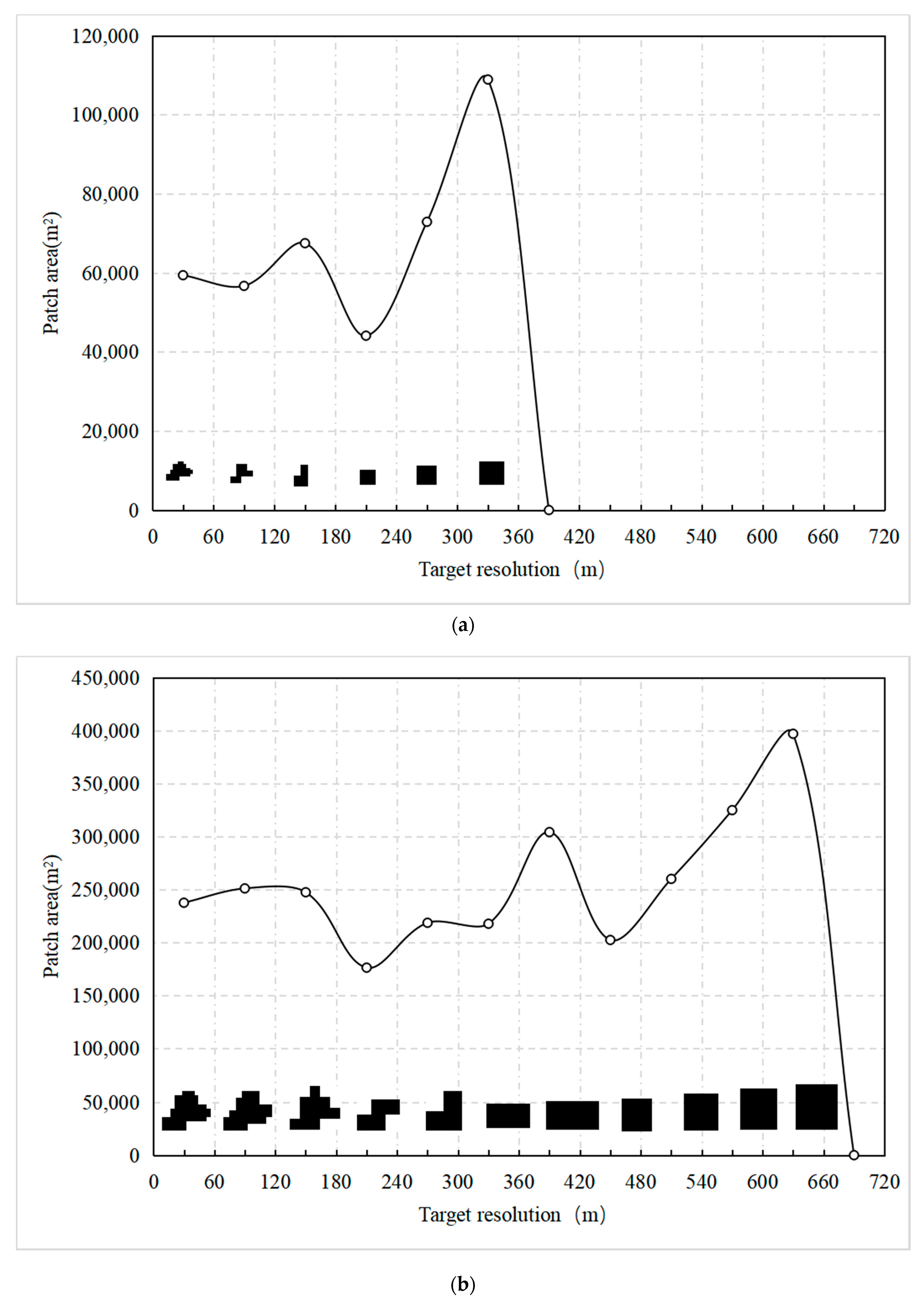
The above analysis can be illustrated with simple experiments. In Figure 1, for the two patches of very similar shape but different size, it is apparent that their area scaling behaviors were similar and the smaller one vanished sooner as expected. In Figure 2, for the two patches of same area but different shape, one compact and one elongated, there was a great difference between their area scaling behaviors. The elongated one gradually diminished almost monotonically while the compact one undulated, lasted much longer, and vanished suddenly. In fact, numerous examples can be found to show that patch area scaling is largely determined by patch morphology, which in this paper refers to patch size and patch shape collectively.
We therefore assume that a patch’s area at a representation resolution is a function of its morphology and the representation resolution, or in formula as:
When inspecting patch area change with resolution, obviously rather than the absolute size it is the relative size of the patch with respect to the representation resolution that matters and plays the primary role. For patches of comparable sizes, the compactness exhibits a significant influence. In addition, to be free from units, patch area at a resolution can be represented by its ratio to the initial value, i.e., area ratio (AR). Formula (1) can thus be transformed to:
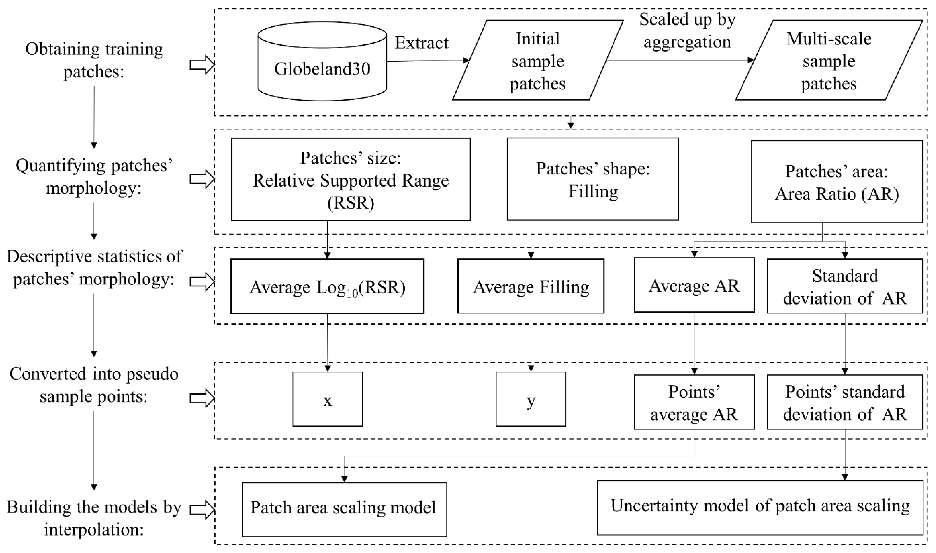
With the above conception and formulation, we model patch area scaling by simply describing the changing of patch area ratio over the patch morphology domain of relative size and compactness with statistics. The overall process of building the patch area scaling model is then as follows: (1) we first find the metrics to quantitatively characterize patch’s relative size and compactness in the next Subsection; (2) and then collect and process sample dataset to statistically describe the patch area scaling and the associated uncertainty. The dataset and its processing methods are described in Section 2.3 together with a processing flow chart.
2.2. Characterizing Patch Morphology
A number of metrics exist that quantify the size and shape of patches [35]. They however are not very suitable for our study of patch scaling. Especially, effective metrics that reflect the resistance of a patch to the discretization effect of representation resolution are still lacking. We therefore propose such a one, namely relative support range, and a supplementary metric of compactness, namely filling, to make the model concise and readily comprehensible. Their definitions, properties and relationship with existing metrics are explained below.
We first define support range (SR) of a patch with Equation (3):
where A is the patch area and P is the patch perimeter.
SR is in fact the width (length of the short side) of a rectangle which has the same A and P as the patch. Therefore, SR essentially indicates the average width of a patch, thus the name support range, when its shape is deemed as a strip that may convolute or branch freely. Regarding SR, it can be observed that: (1) SR is a one-dimensional metric of patch size in the sense that area scales squarely with SR for any shape; (2) for patches of the same shape, the greater SR is, the larger the patch is; (3) for patches of the same area, the larger SR is, the more compact the patch is; (4) SR is a kind of approximation and its performance as a measure of average width will deteriorate when the patch shape goes more and more complicated.
We then define relative support range (RSR) of a patch with Equation (4):
where SR is the support range defined above and R is the representation resolution.
As can be seen, RSR is simply the SR-resolution ratio. Regarding RSR, it can be observed that: (1) RSR measures the one-dimensional size of a patch relative to the resolution and is thus particularly indicative for modeling patch scaling with resolution; (2) if SR can be thought as the width of a patch, RSR can be thought as that width in terms of cell size. Using RSR instead of absolute size metrics for scaling behavior modeling makes compatible the patches with similar shape but different size, and therefore makes the relevant findings independent of the resolution of the sample patches used, i.e., even though the models were built with data of 30 m resolution as explained in the next subsection, they should nevertheless be applicable to data of other resolutions.
As analyzed above, RSR not only is a one-dimensional size metric of a patch but also measures the important narrowness characteristics of patch shape. However, patch shape can be arbitrarily complex. Patches that are indicated by RSR to be narrow and long don’t necessarily extend long and be incompact if they convolute or branch a lot. We therefore supplement RSR with the filling metric so as to better characterize a patch’s compactness, which is considered as the second most important factor that strongly influences patch scaling behavior.
We define filling with Equation (5):
where A is still the patch area and r is the radius of the smallest circumscribing circle of the patch.
Although filling equals one minus the shape metric known as related circumscribing circle, we have it so named to indicate that it stands for the ratio to which a patch fills its smallest circumscribing circle and thus reflects a patch’s overall compactness very well. Apparently, for patches that are indicated narrow and long by RSR, filling can help differentiate the ones that are overall clumpy due to convolution or branching from those that indeed extend long. For calculation simplicity, the smallest circumscribing circle of the minimum bounding box (MBR) of the patch is used instead. So, the theoretical value range of filling is 0~2/π.
2.3. Data and Their Processing
With the patch area scaling model formulated in 2.1 and the needed metrics defined above, we substantiated the model by simply describing the changing of patch area ratio over the RSR-filling domain with statistics. For RSR, its logarithm, Log10(RSR), is used because: (1) while RSR ranges from 0 to positive infinity, its range of main concern is within (0.1~10) as patches of RSR less than 0.1 cannot be represented in general and those with RSR larger than 10 is generally not significantly subject to scale effects; (2) for RSR range of (0.1~10), Log10(RSR) ranges between (−1~1), which is compatible with (0~2/π) of filling. The actual modeling range of Log10(RSR) was set to (−1.56~1.20), which corresponds to (0.03~15.84) of RSR. The actual modeling range of filling was set to its full range, (0~2/π).
Figure 3 shows the flow chart of data processing for building the models. First, initial sample patches were collected. In order to ensure the reliability of modeling results, the number of initial sample patches needs to be large on the one hand, and on the other hand their distribution needs to cover the modeling domain as much as possible. Hence, a huge number of candidate sample patches of 30 m resolution, totalling 1.60 × 10⁷ in number, were extracted from the year-2010 Globeland30 land cover dataset within the geographic extent (72 E–144 E, 20 N–50 N). Globeland30 [36] is the 30-m resolution global land cover data product developed by National Geomatics Center of China (NGCC) and could be downloaded from http://www.globallandcover.com (accessed on 2 December 2020). A subset of the candidate sample patches was then chosen according to their Log10(RSR) and filling to generate the set of initial sample patches. See below for more details of choosing initial sample patches.
Next, the initial sample patches were scaled up by aggregation to a series of coarser resolutions to produce scaled sample patches, and their patch area ratios at each resolution were computed. Fifty resolutions from 90 m to 3030 m with the interval of 60 m were used. Aggregation by majority was adopted to scale initial patches. Each patch was put in a homogenous blank background and aggregated alone. Aggregation was always from the initial patch. Due to the sensitivity of aggregation to start position, each initial patch was aggregated at all possible start positions that make a difference. For scaled patches, RSR was calculated with the initial SR and the current resolution, and filling remained the same because we always aggregate from the initial patch.
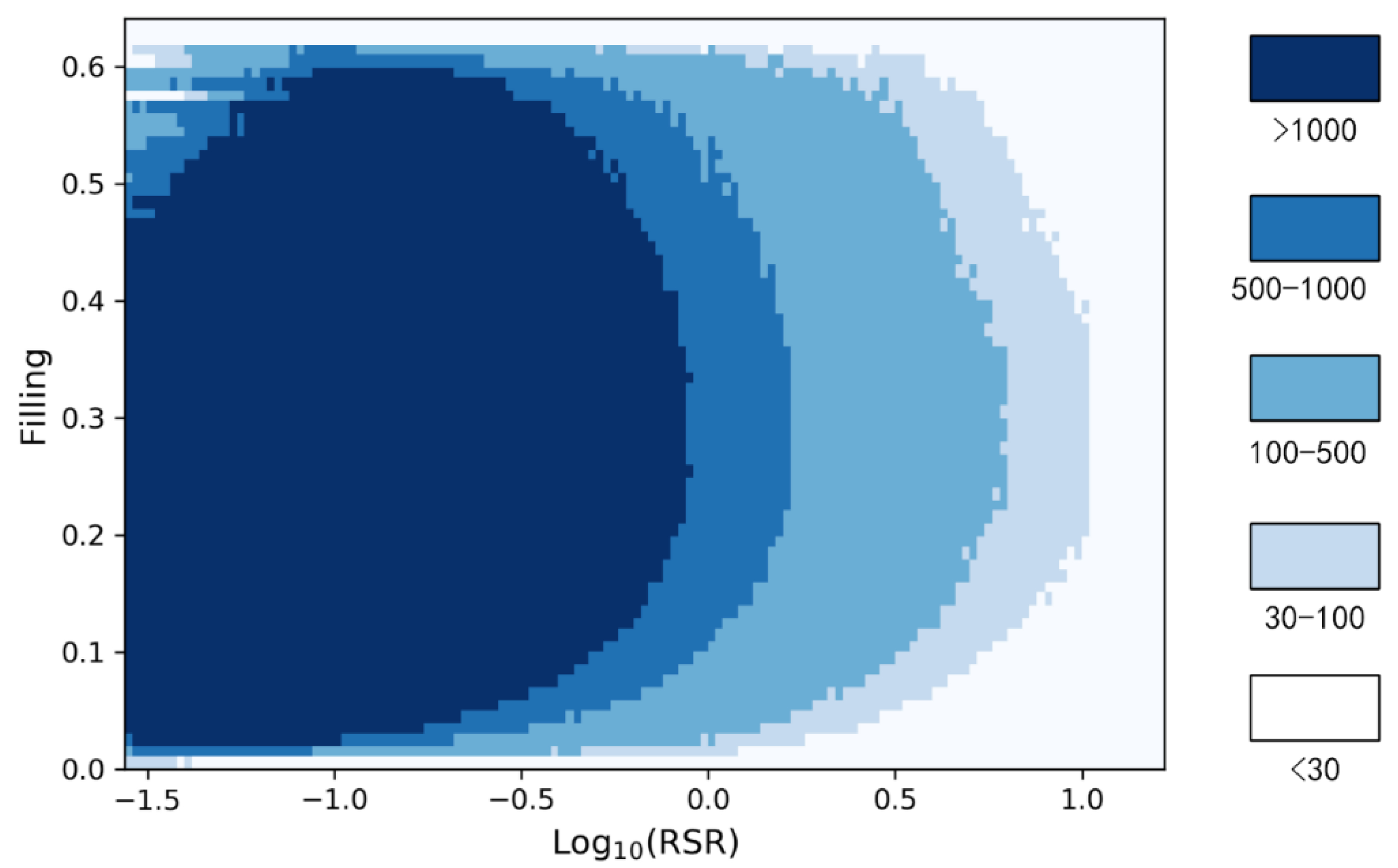
As the number of initial and scaled patches was large, patches of very close morphology were grouped to simplify statistical analysis. Grouping was regularly performed with constant intervals over the (Log10(RSR), filling) domain resulting in a grid of sample groups. The Log10(RSR)-filling domain was gridded into cells of size 0.01*0.01 for grouping sample patches. Sample patches whose Log10(RSR) and filling were within the same cell were taken as a group. For grid cells with more than thirty candidate sample patches, a random subset of thirty was chosen to reduce the sample size. The final distribution of number of sample patches in the Log10(RSR)-filling grid was shown in Figure 4. Each sample group were averaged to generate a pseudo sample point, whose (Log10(RSR), filling) was the centroid of the (Log10(RSR), filling) pairs of the group, area ratio (AR) was the average of the patch area ratios in the group, and AR uncertainty was measured by the standard deviation of the patch area ratios in the group.
Finally, the AR-s and the standard deviations of the pseudo sample points were resampled using ordinary kriging interpolation to produce the grid model of patch area scaling and the associated uncertainty.
3. Results
3.1. The Pair of Models Built
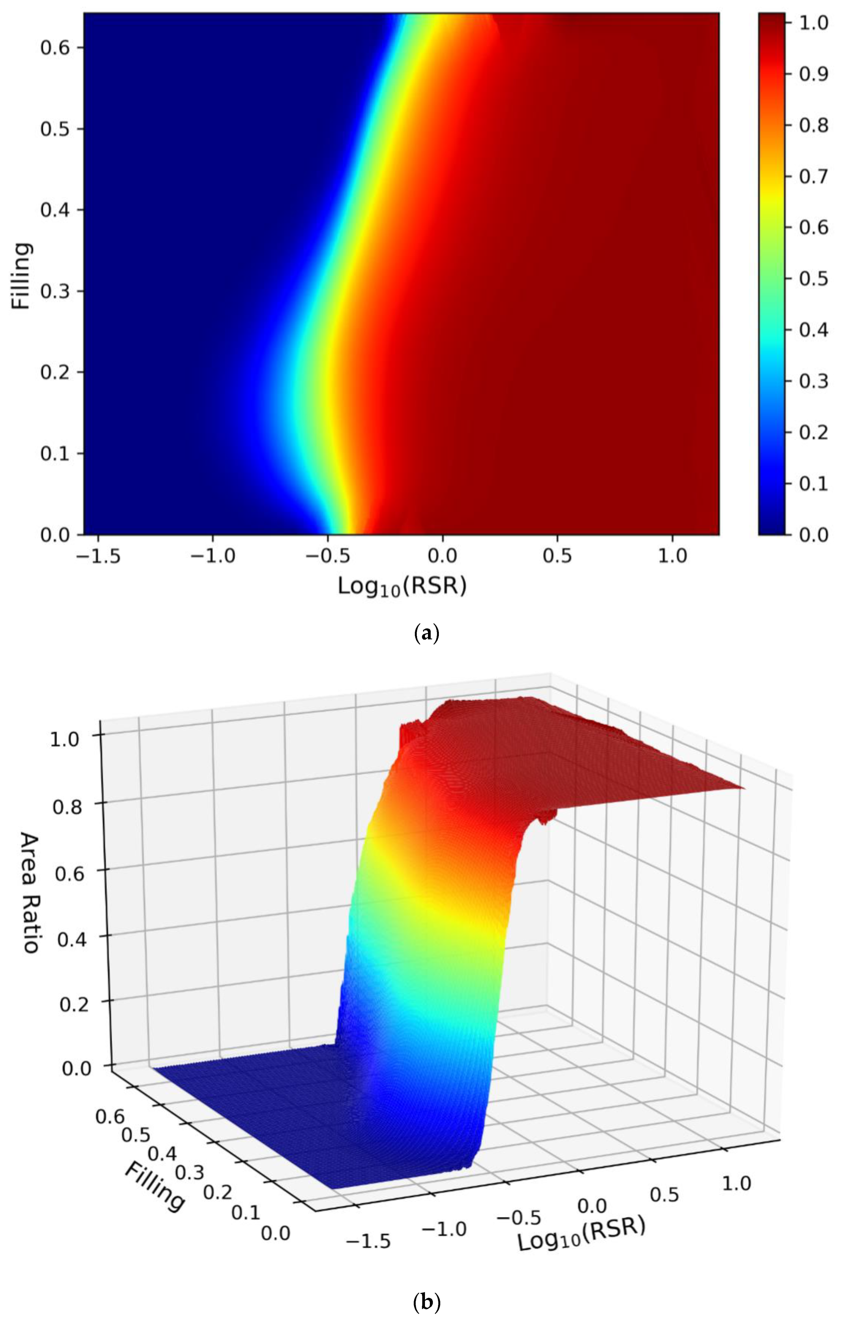
The grid model of patch area scaling built is shown in Figure 5 and that of the uncertainty of patch area scaling is shown in Figure 6. Before making sense of what they tell about patch area scaling, it is worth noting that the models built are complete and detailed in the sense that: (1) they cover the full morphological extent of interest; (2) the scaling model is accompanied by the uncertainty model; (3) they are independent of representation resolution and thus applicable to data of any resolution; (4) they are of high morphological resolution.
The patch area scaling model shown in Figure 5a,b clearly displays a very simple overall pattern of patch area scaling, i.e., patch area ratio changes in a consistent way for all patches in the RSR-filling domain. More specifically, RSR dominates patch area ratio change while filling exhibits the influence of compactness. In fact, the image in Figure 5a suggests that by rotating the axes of RSR and filling, we can even obtain a one-variant model of area ratio scaling for patches of filling greater than 0.2. Given that patch morphology can be arbitrarily complex and different, the existence of such a simple consistent pattern can be surprising. It also indicates the RSR metric indeed characterizes patch area scaling to a great extent while filling is a very good supplement to it, and thus validated our assumptions made in Section 2.1 to some degree.
Some more observations are worth mentioning. Firstly, a range of RSR can be identified with the interval (0.12, 3.16), i.e., (−0.9, 0.5) of Log10(RSR), in which patches diminish gradually till vanishing due to resolution coarsening (the range is called fading range below for brevity). That also means generally patches with RSR larger than 3.16 are not significantly affected (expected AR > 0.98) by the current resolution, and patches with RSR smaller than 0.12 are invisible (expected AR = 0) at the current resolution, and the rest will distort to various extent. In the fading range, the expected patch area decreases almost monotonically with RSR. Secondly, patch compactness significantly influences patch area scaling. Less compact patches are in general more resistant to resolution coarsening in the sense that their area change lags along the RSR axis with respect to compact patches. In addition, compact patches have a much wider fading range than extending ones and vanish much more abruptly than extending ones even though the latter has a much narrower fading range.
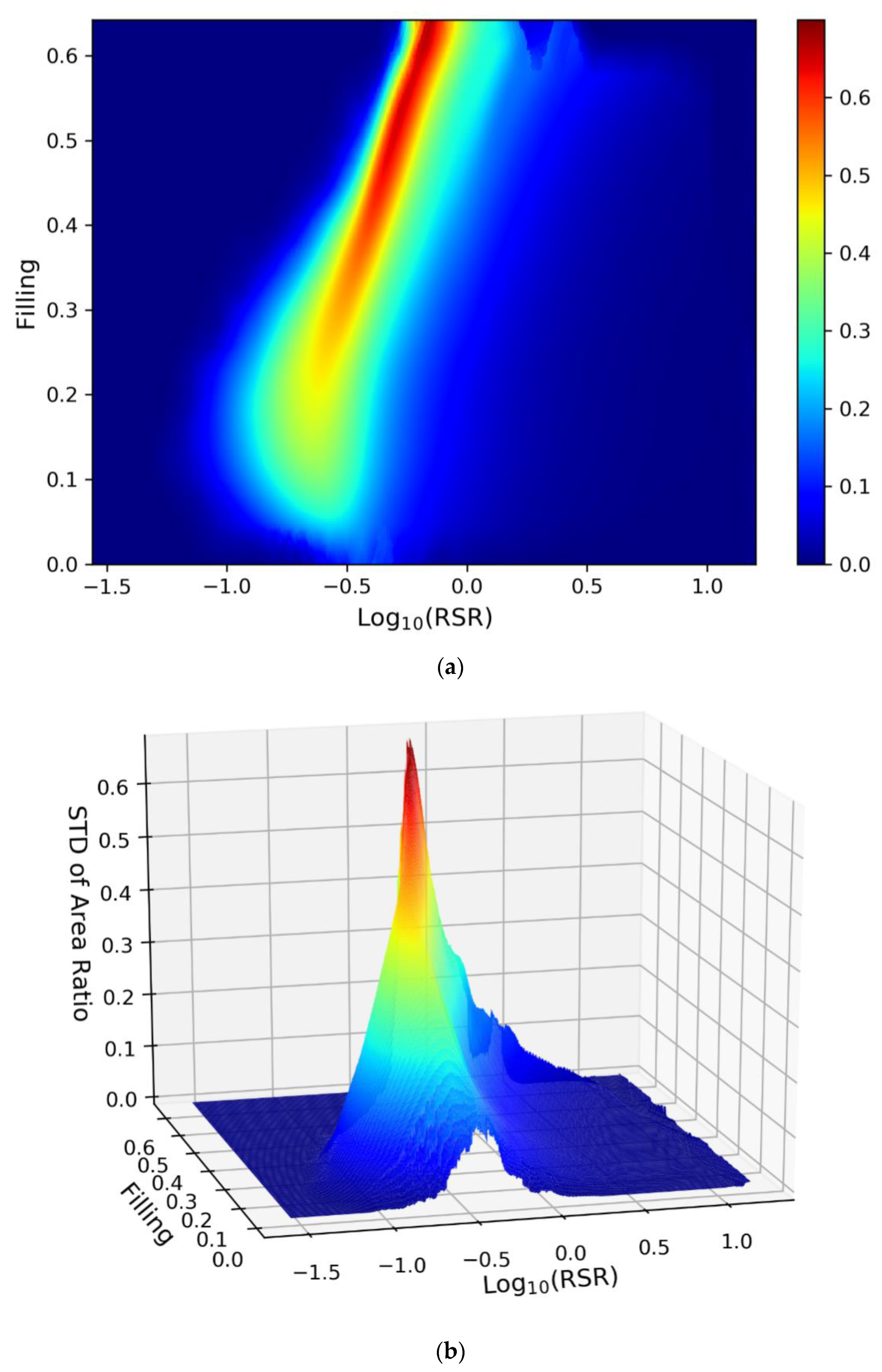
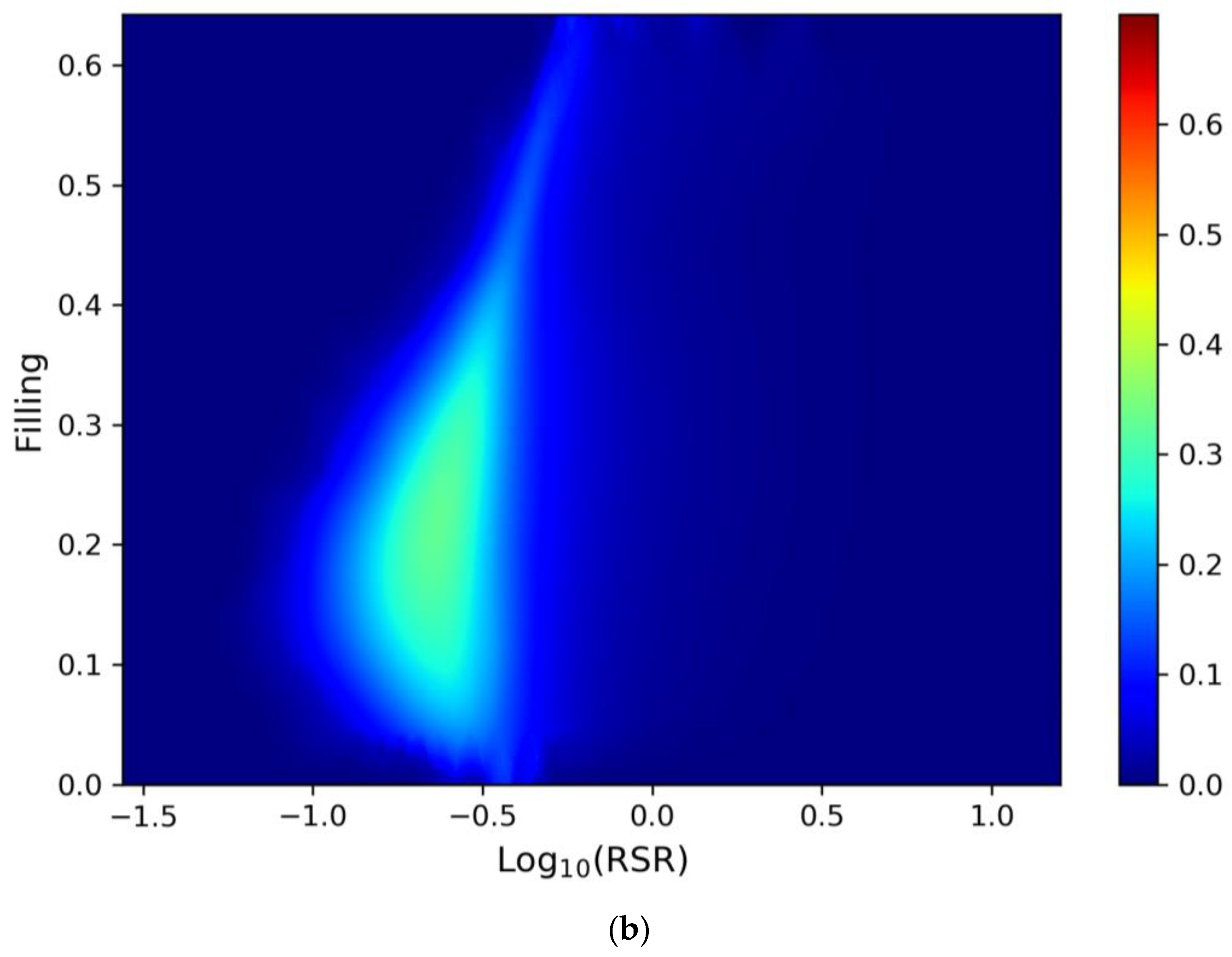
While the area scaling model shows a smooth change of the expectation of area ratio in the fading range, the associated uncertainty model reveals the great uncertainty of area ratio, which can be as large as 0.67 (i.e., 67%) in terms of standard deviation. The overall pattern of uncertainty distribution in the fading range is still simple and looks like a mountain in shape as shown in Figure 6b. There is an apparent ridge line in the mountain-shaped uncertainty distribution as indicated by the color change in Figure 6a and by the surface shape in Figure 6b. The ridge line has its highest value of about 0.67 at the highest filling and its lowest value of about 0.15 when filling approaches zero. That means compact patches has much larger uncertainty than extending ones in the fading range. In addition, for compact patches of filling larger than 0.2, the uncertainty to the right of the ridge line decreases slowly while that to the left decreases quickly. Yet, for extending patches of filling less than 0.2, the uncertainty distribution becomes more and more symmetric around the ridge line as filling decreases to zero.
Again, some details of the uncertainty model are worth noting. When a patch’s RSR is < 0.05 or > 6.31 (i.e., Log10(RSR) < −1.2 or > 0.8 correspondingly), the standard deviation of the patch’s AR is less than 0.02, that is, the patch area scaling has little uncertainty in these RSR ranges. When a patch’s RSR is between 0.05 and 6.31, the standard deviation of patch’s AR varies significantly between 0.02 and 0.67. For the most compact patches, when its RSR is about 0.71 (Log10(RSR) about −0.15 correspondingly), in other words the patch width is 0.71 of the representation resolution, the uncertainty of patch area scaling reaches the maximum. That is because in such situation the representability of a patch is extremely sensitive to its position relative to the cells. For less compact patches, such phenomenon also exists but the peak value shifts leftwards. That is likely due to that RSR is only an assumed average width of patches and its validity deteriorates gradually when patch morphology goes more and more complex.
3.2. Verifying the Models by Predicting Patch Area Scaling
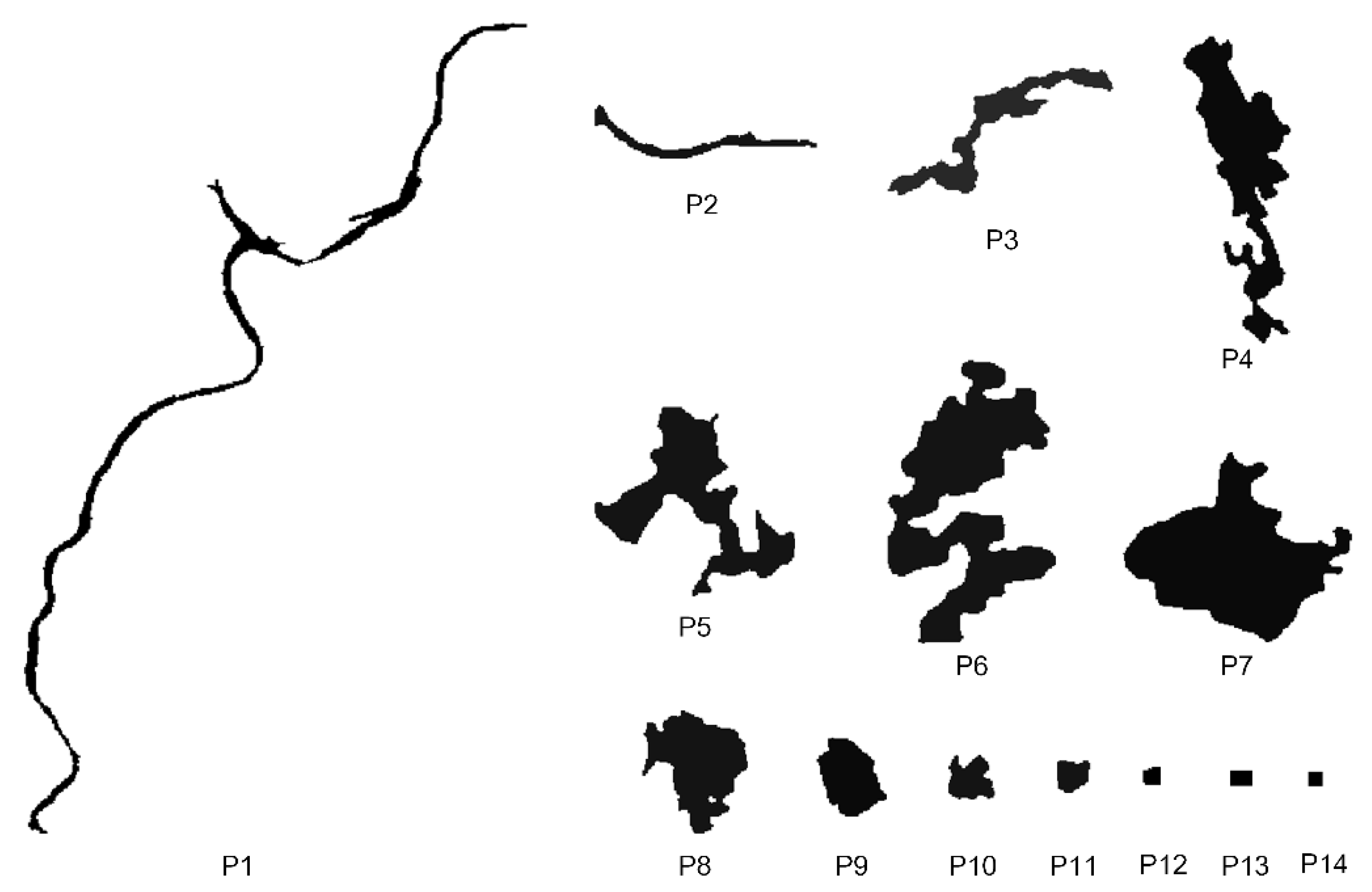
As the models built are complete and detailed, they should then be able to tell in advance the area scaling behavior of any patch reasonably well. Fourteen representative patches of very different morphology were selected to demonstrate the usage and verify the models. They are shown in Figure 7 and numbered from P1 to P14. Their morphological metrics are listed in Table 1. As can be seen from Figure 7 and Table 1, the patches are in general getting more compact and less complex with the increase of filling from P1 to P14.
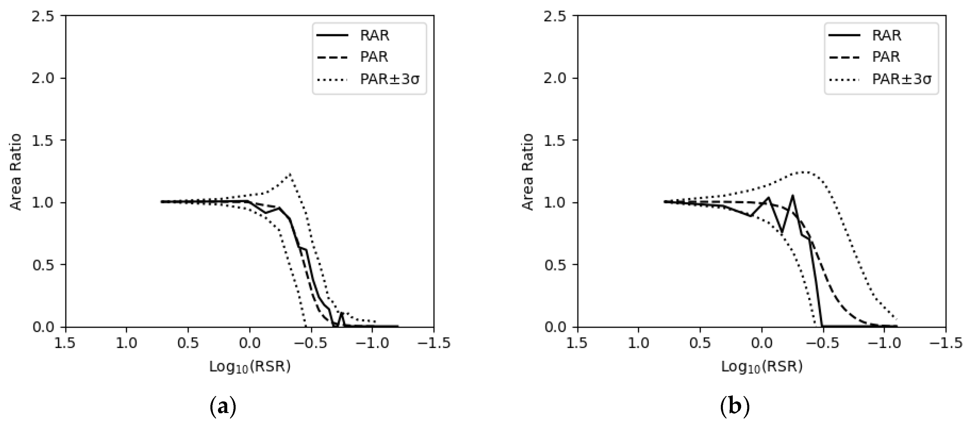
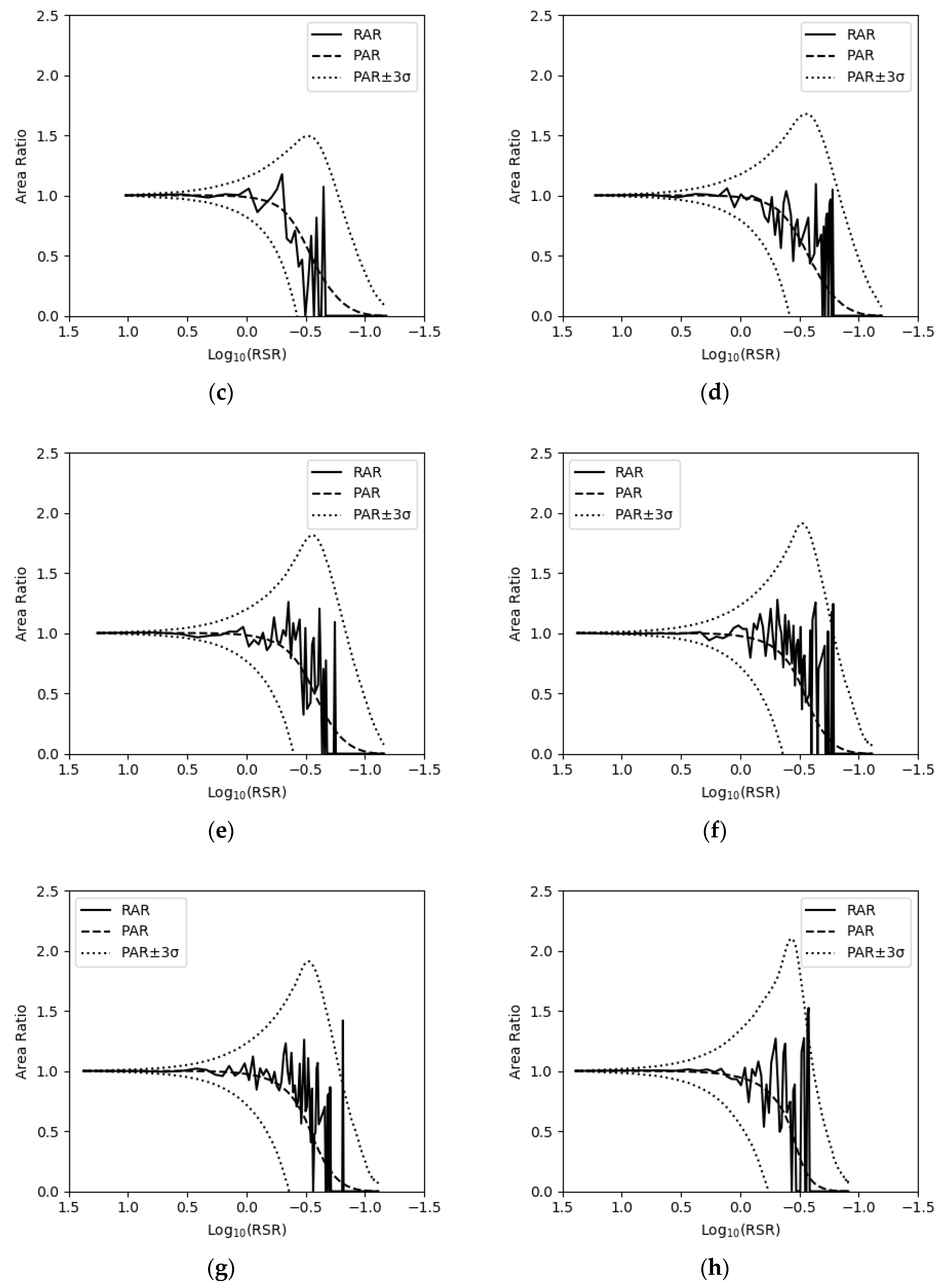
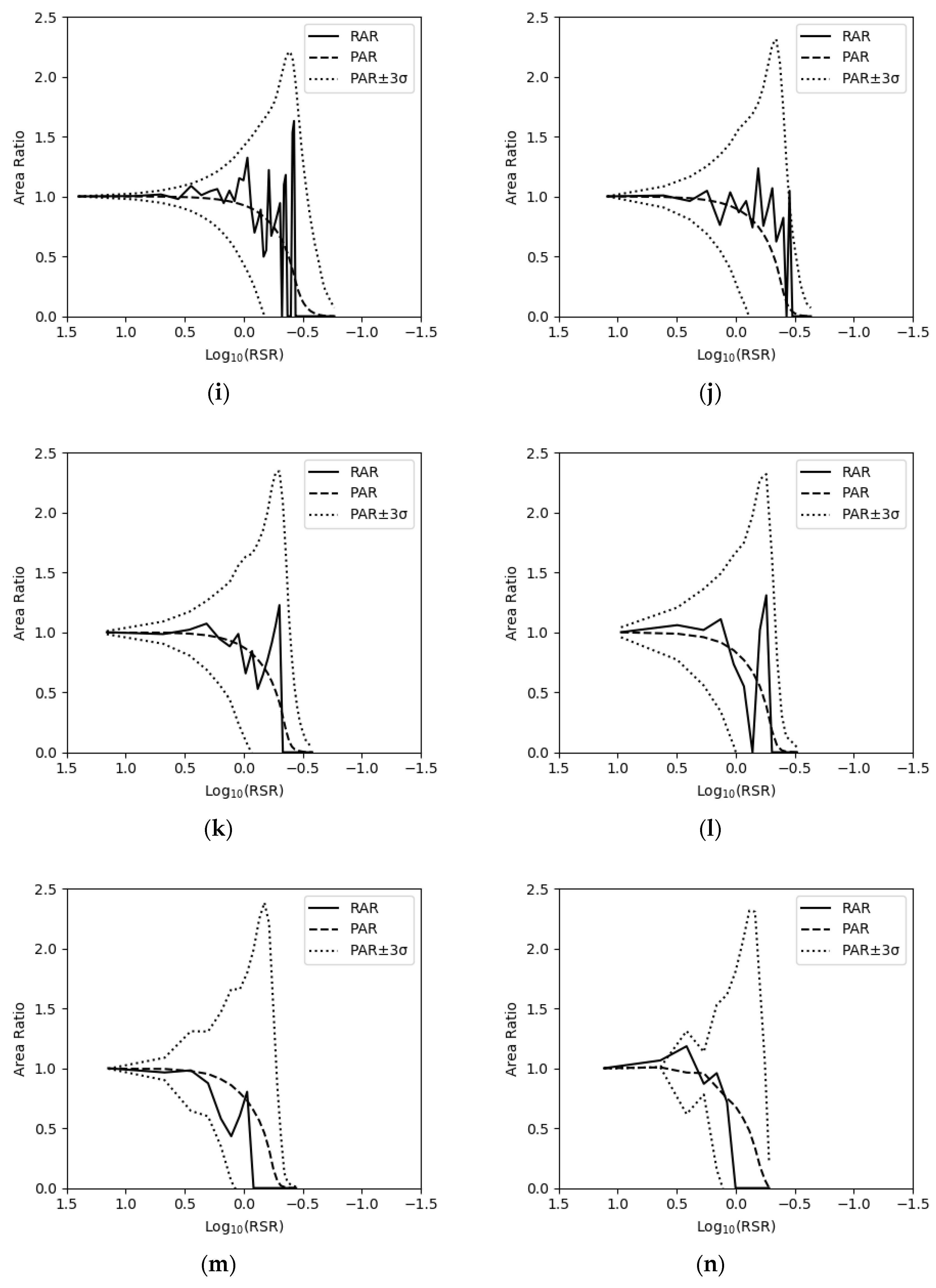
In Figure 8, plotted at a series of resolutions are their real area ratio (RAR), predicted area ratio (PAR) and PAR ± 3σ. The PAR values were obtained by looking up in the patch area scaling model, and σ, the standard deviation of PAR, were obtained by looking up in the uncertainty model. Patch’s RAR was obtained at a random start position of aggregation at each resolution. As can be seen, the overall tendency of RAR and PAR matches well for all the patches and their difference are within 3σ in most cases. In addition, the difference between RAR and PAR varies synchronously with σ along the resolution axis. Therefore, these cases demonstrated that both the scaling and the uncertainty models are valid.
3.3. Applying the Patch Area Scaling Model to Predict Class Area Scaling
As reviewed in the Introduction, it has long been desired to uncover the scaling behavior of the area of a certain LULC class in environmental analysis. As a further verification of the patch area scaling model built and a demonstration of its potential usage, we show here the basic feasibility to use it to predict class area scaling.
At the landscape level, however, the class composition and spatial configuration factors will manifest themselves in aggregation [37] and their working mechanisms demand separate studies. We therefore consider only the single-class landscape in this study and assume that patches are so apart from each other that their interaction in aggregation can be neglected. Under such simplification, class area scaling can be predicted by simply summing up patch area scaling.
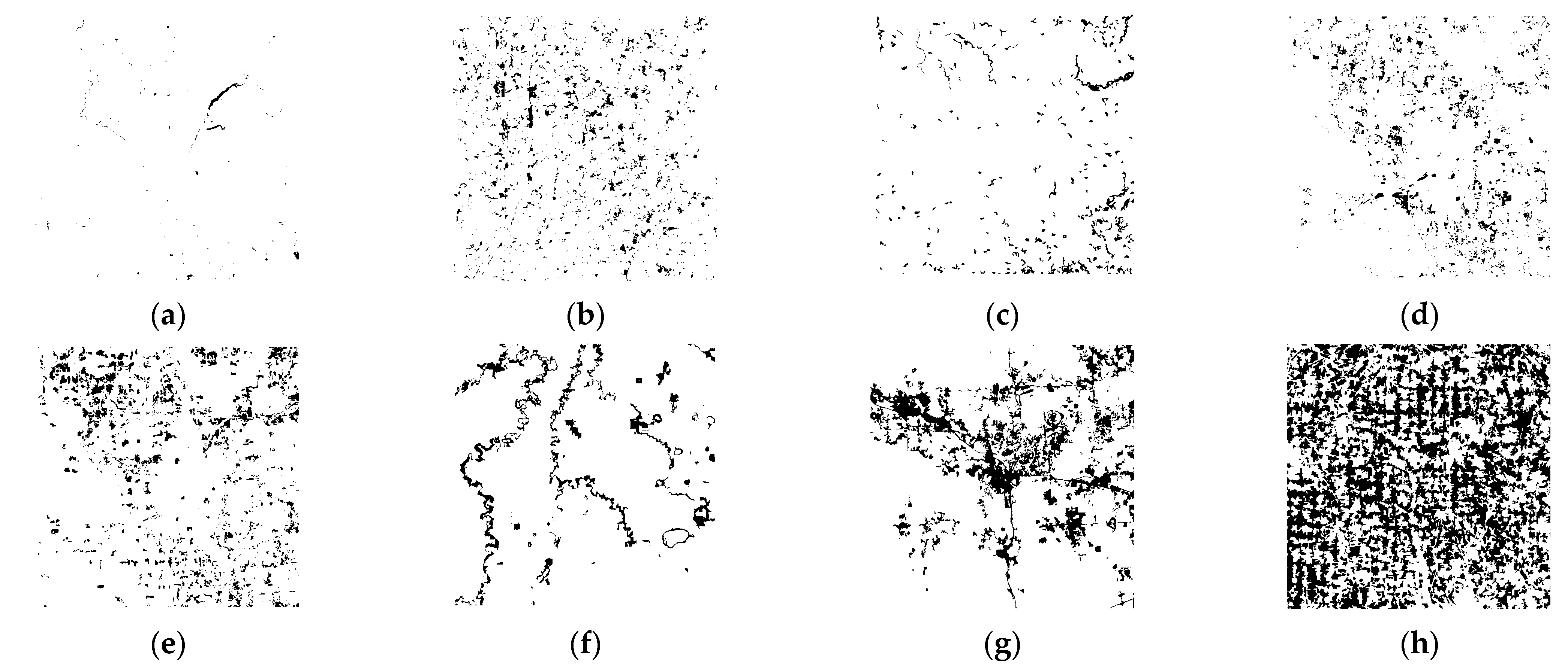
Eight single-class landscapes of different spatial patterns were selected to evaluate the feasibility and performance of predicting class area scaling. The test landscapes are shown in Figure 9 and numbered from C1 to C8. They are all real-world landscapes extracted from GlobalLand30 of 50 km × 50 km extent. Statistics of them are listed in Table 2. As can be seen from Figure 9, patches are gradually getting larger and closer to each other from C1 to C8. Therefore, it is anticipated that our simple method of predicting class area scaling should work for some of the landscapes and fail for others.
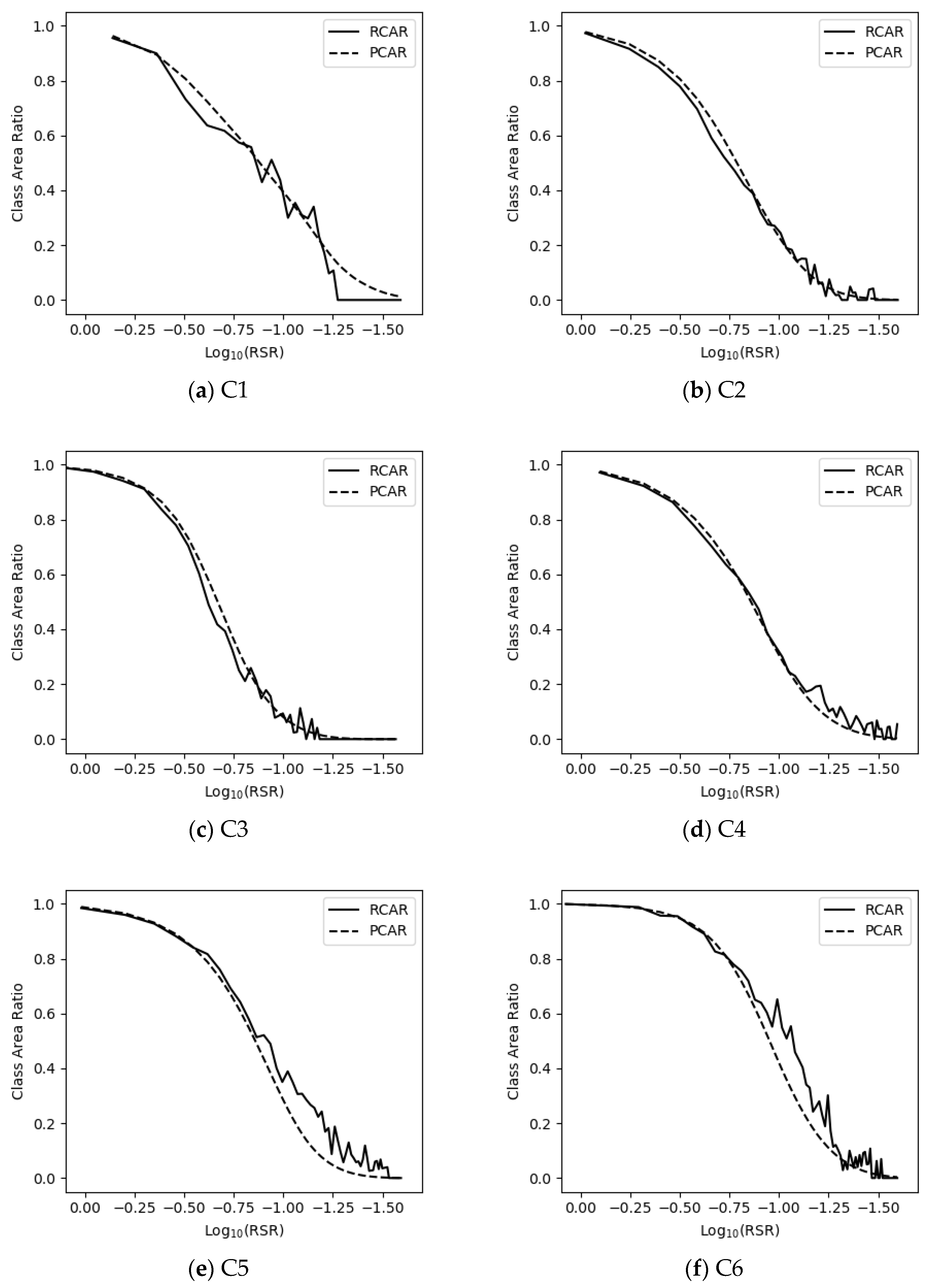
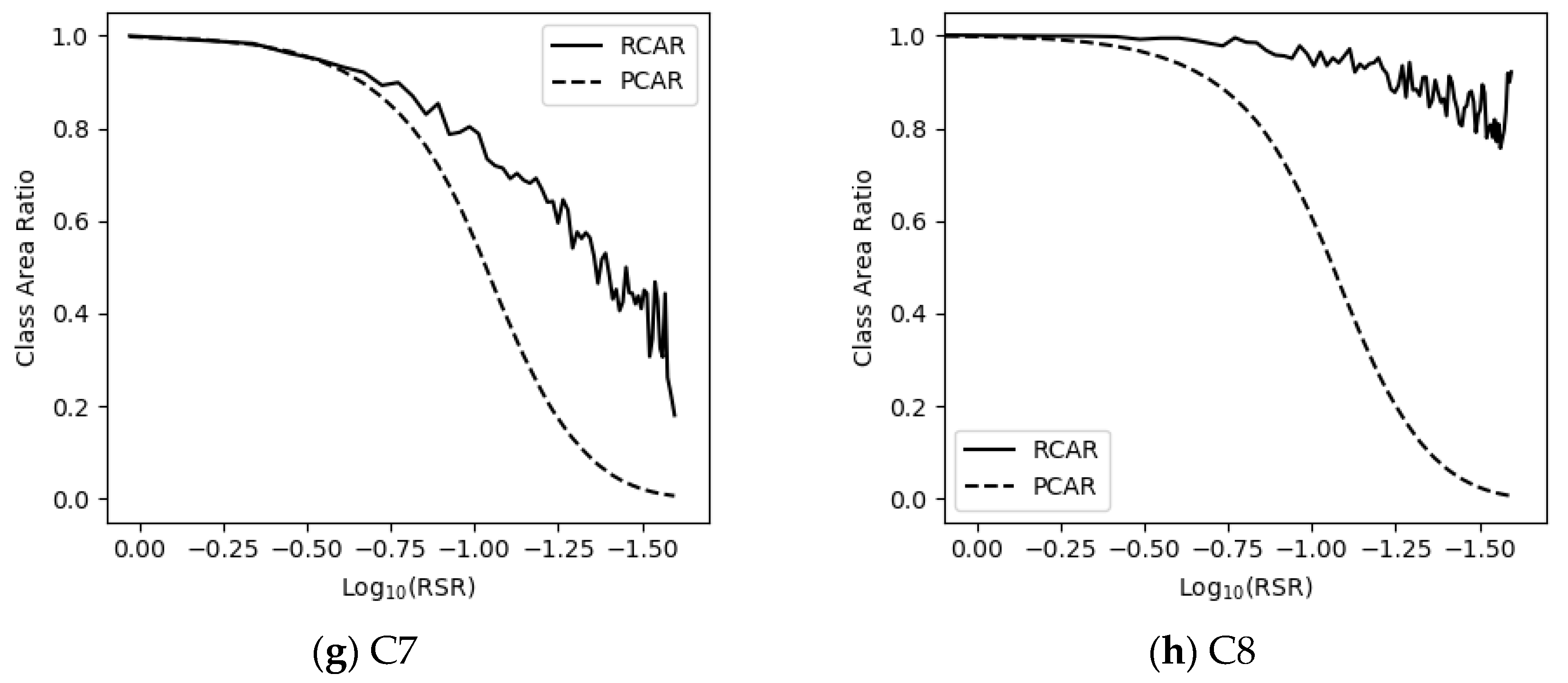
The test landscapes were constantly scaled up until their real class areas ratio (RCAR) and/or predicted class area ratio (PCAR) became zero. Their predicted and real area scaling behaviors are plotted in Figure 10, in which the Log10(RSR) value was the average of all patches in the landscape at a certain resolution. As can be seen, for C1 to C6, class area scaling was predicted quite well as the assumption of dispersive distribution of patches held approximately. That was especially true for C1-C4. Generally, the better the assumption held, the better the prediction was. The prediction error was less than 0.1 (i.e., 10%) in most cases and almost always less than 0.2 in terms of the ratio to initial class area. For the exceptional cases of C7 and C8, it is apparent that our assumption about patch distribution was seriously violated. It can thus be concluded that it is basically possible to predict class area scaling by synthesizing patch area scaling although further study is required to take into account the effects of landscape configuration and composition.
4. Discussions
In the process of building the models, it was found that alternative choices of patch morphological metrics may be used. In addition, the modeled uncertainty included the influence of incomplete characterization of patch morphology with the metrics. We give some discussions on these issues for possible improvement in future study.
4.1. Selection of Metrics for Charactering Patches’ Morphology
Quantifying patch morphology plays a key role in building the patch area scaling model and its uncertainty model. Up to now, there have been many metrics for describing patch morphology [35], mainly including radius of gyration (GYRATE), perimeter-area ratio (PARA), area-perimeter ratio (RAPA), shape index (SHAPE), compactness index (COMPACT), related circumscribing circle (RCC), fractal dimension index (FRAC). In order to select suitable metrics for describing patch morphology from existing and our proposed metrics, i.e., support range (SR) and filling, a correlation analysis and a principal component analysis were conducted [38]. It was found that the combination of GYRATE and SR as the most significant component had a slightly higher variance contribution than that of SR and filling, meaning they may capture more morphological information than the pair we used. Given the close statistic performance of the two pairs, we took into account of model interpretability in making the choice. As we know, two basic elements of patch morphology are the size and the shape. However, both GYRATE and SR are inclined to describe patch size, leaving patch shape less covered. That made us use filling, a patch shape metric, to pair RSR in place of GYRATE in this study. Nevertheless, in future research, GYRATE and SR still can be considered for building the models.
4.2. Inherent Uncertainty of Patch Area Scaling and That Resulting from Modeling Approximation
In Section 3.1, the uncertainty model of patch area scaling model was presented. It should be noted that there were two sources of uncertainty in our modeling. One resulted from the inherent randomness of grid-patch alignment due to rasterization, and the other from the approximation of using the two metrics, i.e., RSR and filling, to characterize patch morphology. In order to clarify their contribution to the observed uncertainty, we estimated them separately. For each sample patch in each of the morphology grid cell specified in Section 2.3, the average and the standard deviation of the area ratios obtained at different start positions of aggregation were first calculated. Then, for each cell, the standard deviation of the area ratios of different patches were averaged (denoted by a_sd_ar for short) as the estimation of the uncertainty resulting from random rasterization, which is plotted in Figure 11a. Similarly, the standard deviation of the averages of area ratios of different patches (denoted by sd_a_ar for short) was calculated as the estimation of the uncertainty resulting from modeling approximation, which is plotted in Figure 11b. By comparing them, it can be found that for patches of filling greater than 0.3, a_sd_ar is much larger than sd_a_ar, and, for patches of filling less than 0.3, a_sd_ar gradually decreases and becomes roughly equal to sd_a_ar when filling is less than 0.2. That means the uncertainty shown in Figure 6 resulted largely from the inherent randomness in rasterization although the approximation made in our modeling did have a share.
5. Conclusions
A complete patch area scaling model was built in this study, which demonstrates the existence of a simple consistent pattern of scaling with RSR for all patches, and the filling-dependent fading range of different patches. This is, to our knowledge, the first time that the scaling behavior of a spatial analysis metric was systematically modeled. That was made possible through an analytics and descriptive statistics-combined approach. The analytical part first conceptually formulated the functional relation between resolution-dependent patch area and patch morphology, the latter of which was quantitatively measured by the proposed metrics of relative support range and filling. The descriptive statistics part substantiated the functional relation as a gridded surface with a vast number of sample patches that almost fully covered the scaling domain of concern.
This study made an important distinction between the certain and the uncertain components of what was indistinctively called scale effect in the literature and provided an uncertainty model accompanying the scaling model. The certain part represents the trend and can largely be predictable when the resolution becomes coarser, and thus seems to be what we want to mean by the term of scale effect. In contrast, the uncertain part is largely due to the randomness in discretization and not predictable, and thus may be more properly called scale uncertainty. Unfortunately, as can be seen from the model built and the cases studied, the uncertain part can often be larger than or comparable with the certain part in magnitude. That warns us to clarify the cause before taking scale effects as certain.
The models built are readily usable for a number of purposes. The scaling model as demonstrated can serve as a lookup table to know in advance the area scaling behavior of any patch of any resolution. It can also be used to scale up patch areas when comparing results of different resolutions. The fading range indicates that a patch is almost free from scale effect only when its RSR is larger than 6.31 and thus provides a basis for choosing a proper data resolution for a study. Correspondingly, the uncertainty model as demonstrated can serve as a lookup table to know in advance the area uncertainty of any patch of any resolution. Another important use of the uncertainty model could be, when interpreting scale effects on patch areas, to help us make sure it is the certain part of scale effects when the corresponding uncertainty is small enough. Maybe, the most important use of the models is for predicting class area scaling by analytical synthetization. To demonstrate that idea, a simple method of summarizing patches’ behavior was proposed to synthesize class area scaling under the dispersive distribution assumption for single-class landscapes, and applied to eight cases. It turned out to perform reasonably well when the assumption held to a reasonable extent.
Extension to this works is considered possible and promising. On the one hand, the hybrid approach to modeling patch area scaling is thought applicable to modeling other patch level metrics, such as perimeter, radius of gyration, and largely those based on patch area and perimeter. With more and more patch level metrics modeled, patch scaling can be decrypted. On the other hand, the synthesizing approach to studying class and landscape levels’ scale effects on raster categorical data can be extended by taking into account the influence of landscape composition and configuration [1,37], thereby making higher level scaling behavior analytically modeled in a bottom-up way. It is considered feasible given the intensive researches done on class and landscape level metrics [39,40].
Author Contributions
Conceptualization, Q.Z. and Z.X.; methodology, Q.Z. and Z.X.; validation, Q.Z.; formal analysis, Q.Z. and Z.X.; resources, Z.X.; writing—original draft preparation, Q.Z.; writing—review and editing, Z.X.; visualization, Q.Z.; supervision, Z.X.; project administration, Z.X.; funding acquisition, Z.X. All authors have read and agreed to the published version of the manuscript.
Funding
This research was funded by National Natural Science Foundation of China, grant number 41971330.
Data Availability Statement
The data that support the findings of this study were derived from the following resources available in the public domain: http://www.globallandcover.com/ (accessed on 2 December 2020).
Acknowledgments
We would like to thank National Geomatics Center of China for providing Globeland30 data (http://www.globallandcover.com/ (accessed on 2 December 2020)).
Conflicts of Interest
The authors declare no conflict of interest.
References
- Turner, M.G.; O’Neill, R.V.; Milne, G.B.T. Effects of changing spatial scale on the analysis of landscape pattern. Landsc. Ecol. 1989, 3, 153–162. [Google Scholar] [CrossRef]
- Openshaw, S. A geographical solution to scale and aggregation problems in region-building, partitioning and spatial modelling. Trans. Inst. Br. Geogr. 1977, 2, 459–472. [Google Scholar] [CrossRef]
- Lam, S.N.; Quattrochi, D.A. On the Issues of Scale, Resolution, and Fractal Analysis in the Mapping Sciences. Prof. Geogr. 1992, 44, 88–98. [Google Scholar] [CrossRef]
- Chen, Y.; Zhou, Q. A scale-adaptive DEM for multi-scale terrain analysis. Int. J. Geogr. Inf. Sci. 2013, 27, 1329–1348. [Google Scholar] [CrossRef]
- Sposito, G. Scale Dependence and Scale Invariance in Hydrology; Cambridge University Press: Cambridge, UK, 1998. [Google Scholar]
- Luan, H.J.; Tian, Q.J.; Yu, T.; Hu, X.L.; Huang, Y.; Du, L.T.; Zhao, L.M.; Wei, X.; Han, J.; Zhang, Z.W. Modeling Continuous Scaling of NDVI Based on Fractal Theory. Spectrosc. Spectr. Anal. 2013, 33, 1857–1862. [Google Scholar]
- Dong, L.; Liu, H.; Riffat, S. Development of small-scale and micro-scale biomass-fuelled CHP systems—A literature review. Appl. Ther. Eng. 2009, 29, 2119–2126. [Google Scholar] [CrossRef] [Green Version]
- Sandel, B. Towards a taxonomy of spatial scale-dependence. Ecography 2015, 38, 358–369. [Google Scholar] [CrossRef]
- Goodchild, M.F. Scale in GIS: An overview. Geomorphology 2011, 130, 5–9. [Google Scholar] [CrossRef]
- Li, X.; Wang, J.; Strahler, A.H. Scale effects and scaling-up by geometric-optical model. Sci. China Ser. E 2000, 43, 17–22. [Google Scholar] [CrossRef]
- Moody, A.; Woodcock, C. Scale-Dependent Errors in the Estimation of Land-Cover Proportions: Implications for Global Land-Cover Datasets. Photogramm. Eng. Remote Sens. 1994, 60, 585–596. [Google Scholar]
- Woodcock, C.E.; Strahler, A.H. The factor of scale in remote sensing. Remote Sens. Environ. 1987, 21, 311–332. [Google Scholar] [CrossRef]
- Wu, J. Effects of changing scale on landscape pattern analysis: Scaling relations. Landsc. Ecol. 2004, 19, 761–782. [Google Scholar] [CrossRef]
- Jones, H.G.; Sirault, X.R.R. Scaling of Thermal Images at Different Spatial Resolution: The Mixed Pixel Problem. Agronomy 2014, 4, 380–396. [Google Scholar] [CrossRef] [Green Version]
- Wu, J.; Jones, K.; Li, H.; Loucks, O. Scaling and Uncertainty Analysis in Ecology: Methods and Applications; Springer: New York, NY, USA, 2006; ISBN 1-4020-4662-6. [Google Scholar]
- Gallo, K.P.; Easterling, D.R.; Peterson, T.C. The influence of land use/land cover on climatological values of the diurnal temperature range. J. Clim. 1996, 9, 163–165. [Google Scholar] [CrossRef] [Green Version]
- Kindu, M.; Schneider, T.; Döllerer, M.; Teketay, D.; Knoke, T. Scenario modelling of land use/land cover changes in Munessa-Shashemene landscape of the Ethiopian highlands. Sci. Total Environ. 2018, 622–623, 534–546. [Google Scholar] [CrossRef]
- Mahmood, R.; Pielke, R.A., Sr.; Hubbard, K.G.; Yogi, D.N.; Syktus, J. Impacts of Land Use/Land Cover Change on Climate and Future Research Priorities. Bull. Am. Meteorol. Soc. 2010, 91, 37–46. [Google Scholar] [CrossRef]
- Bhagawat, R.; Zhang, L.; Hamidreza, K.; Barry, H.; Sushila, R.; Zhang, P. Land Use/Land Cover Dynamics and Modeling of Urban Land Expansion by the Integration of Cellular Automata and Markov Chain. ISPRS Int. J. Geo Inf. 2018, 7, 154. [Google Scholar]
- Baidya Roy, S.; Avissar, R. Impact of land use/land cover change on regional hydrometeorology in Amazonia. J. Geophys. Res. Atmos. 2002, 107, 8037. [Google Scholar] [CrossRef] [Green Version]
- Pielke, R., Sr.; Pitman, A.; Niyogi, D.; Mahmood, R.; Mcalpine, C.; Hossain, F.; Klein Goldewijk, K.; Nair, U.; Betts, R.; Fall, S.; et al. Land use/land cover changes and climate: Modeling analysis and observational evidence. Wiley Interdiscip. Rev. Clim. Chang. 2011, 2, 828–850. [Google Scholar] [CrossRef]
- Turner, B.L., II; Meyer, W.B.; Skole, D.L. Global land-use/land-cover change: Towards an integrated study. Integr. Earth Syst. Sci. 1994, 23, 91–95. [Google Scholar] [CrossRef]
- Etienne, R.S. On optimal choices in increase of patch area and reduction of interpatch distance for metapopulation persistence. Ecol. Model. 2015, 179, 77–90. [Google Scholar] [CrossRef]
- Ferraz, G.; Nichols, J.D.; Hines, J.E.; Stouffer, P.C.; Bierregaard, R.O.; Lovejoy, T.E. A Large-Scale Deforestation Experiment: Effects of Patch Area and Isolation on Amazon Birds. Science 2007, 315, 238–241. [Google Scholar] [CrossRef] [Green Version]
- Hambäck, P.; Englund, G. Patch area, population density and the scaling of migration rates: The resource concentration hypothesis revisited. Ecol. Lett. 2005, 8, 1057–1065. [Google Scholar] [CrossRef]
- Honnay, O.; Endels, P.; Vereecken, H.; Hermy, M. The role of patch area and habitat diversity in explaining native plant species richness in disturbed suburban forest patches in northern Belgium. Biodivers. Res. 1999, 5, 129–141. [Google Scholar] [CrossRef]
- Landeiro, V.L.; Hamada, N.; Godoy, B.S.; Melo, A.S. Effects of litter patch area on macroinvertebrate assemblage structure and leaf breakdown in Central Amazonian streams. Hydrobiologia 2010, 649, 355–363. [Google Scholar] [CrossRef]
- Muad, A.; Foody, G. Impact of Land Cover Patch Size on the Accuracy of Patch Area Representation in HNN-Based Super Resolution Mapping. IEEE J. Sel. Top. Appl. Earth Obs. Remote Sens. 2012, 5, 1418–1427. [Google Scholar] [CrossRef] [Green Version]
- Schtickzelle, N.; Baguette, M. Behavioural responses to habitat patch boundaries restrict dispersal and generate emigration–patch area relationships in fragmented landscapes. J. Anim. Ecol. 2003, 72, 533–545. [Google Scholar] [CrossRef] [PubMed]
- Evans, P. Scaling and assessment of X-ray data quality. Acta Cryst. D. Biol. Cryst. 2006, 62, 72–82. [Google Scholar] [CrossRef]
- Finke, P.A.; Bierkens, M.F.P.; Willigen, P. Choosing Appropriate Upscaling and Downscaling Methods for Environmental Research; IAHS: Wallingford, UK, 2002. [Google Scholar]
- Zhang, W.; Li, T.; Huang, Y.; Zhang, Q.; Bian, J.; Han, P. Estimation of uncertainties due to data scarcity in model upscaling: A case study of methane emissions from rice paddies in China. Geosci. Model Dev. Discuss. 2014, 7, 181–216. [Google Scholar]
- Lechner, A.M.; Stein, A.; Jones, S.D.; Ferwerda, J.G. Remote sensing of small and linear features: Quantifying the effects of patch size and length, grid position and detectability on land cover mapping. Remote Sens. Environ. 2009, 113, 2194–2204. [Google Scholar] [CrossRef]
- Tan, S.; Xu, Z.; Ti, P.; Li, Z. Morphology-based modeling of aggregation effect on the patch area size for GlobeLand30 data. Trans. GIS 2018, 22, 98–118. [Google Scholar] [CrossRef]
- Mcgarigal, K.S.; Cushman, S.A.; Neel, M.C.; Ene, E. FRAGSTATS: Spatial Pattern Analysis Program for Categorical Maps; University of Massachusetts Amherst: Amherst, MA, USA, 2002. [Google Scholar]
- Chen, J.; Ban, Y.; Li, S. China: Open access to Earth land-cover map. Nature 2014, 514, 434. [Google Scholar]
- Qi, Y.; Wu, J. Effects of changing spatial resolution on the results of landscape pattern analysis using spatial autocorrelation indices. Landsc. Ecol. 1996, 11, 39–49. [Google Scholar] [CrossRef]
- Zhang, Q.; Tan, S.; Xu, Z.; Huang, Z. Applicability and simplification study of patch level landscape metrics based on GLC30. Remote Sens. L. Resour. 2017, 029, 98–105. [Google Scholar] [CrossRef]
- Gustafson, E.J. Quantifying landscape spatial pattern: What is the state of the art? Ecosystems 1998, 1, 143–156. [Google Scholar] [CrossRef]
- Lausch, A.; Salbach, C.; Schmidt, A.; Doktor, D.; Pause, M. Deriving phenology of barley with imaging hyperspectral remote sensing. Ecol. Model. 2015, 295. [Google Scholar] [CrossRef]
Figure 1.
The area scaling behaviors of a pair of similar patches of different area. (a) The area scaling of the smaller patch; (b) The area scaling of the bigger patch. The initial patch at 30 m resolution (a) was extracted from the year-2010 Globeland30 data, and the initial patch in (b) was generated by magnifying that of (a) four times. For other resolutions, the patches were obtained by aggregating the initial patches.

Figure 2.
The area scaling behaviors of a pair of dissimilar patches of the same area. (a) The area scaling of an elongated patch; (b) The area scaling of a compact patch. The initial patches at 30 m resolution in (a,b) were extracted from the year-2010 Globeland30 data. For other resolutions, the patches were obtained by aggregating the initial patches.

Figure 3.
The flow chart of building the patch area scaling model and its uncertainty model. Globeland30 is the 30-m resolution global land cover data product developed by NGCC and could be downloaded from http://www.globallandcover.com (accessed on 2 December 2020).
Figure 3.
The flow chart of building the patch area scaling model and its uncertainty model. Globeland30 is the 30-m resolution global land cover data product developed by NGCC and could be downloaded from http://www.globallandcover.com (accessed on 2 December 2020).

Figure 4.
The distribution of number of sample patches in the Log10(RSR)-filling grid.

Figure 5.
The patch area scaling model in 2- and 3-dimentional views. (a) A two-dimensional view of the patch area scaling model; (b) A three-dimensional view of the patch area scaling model.
Figure 5.
The patch area scaling model in 2- and 3-dimentional views. (a) A two-dimensional view of the patch area scaling model; (b) A three-dimensional view of the patch area scaling model.

Figure 6.
The uncertainty model of patch area scaling in 2- and 3- dimensional views. (a) A two-dimensional view of the uncertainty model; (b) A three-dimensional view of the uncertainty model.
Figure 6.
The uncertainty model of patch area scaling in 2- and 3- dimensional views. (a) A two-dimensional view of the uncertainty model; (b) A three-dimensional view of the uncertainty model.

Figure 7.
The representative test patches.

Figure 8.
The predicted and real area scaling behaviors of the test patches (RAR stands for real area ratio. PAR stands for predicted area ratio. σ stands for the standard deviation of PAR given by the uncertainty model.). (a) P1; (b) P2;(c) P3; (d) P4; (e) P5; (f) P6; (g) P7; (h) P8; (i) P9; (j) P10; (k) P11; (l) P12; (m) P13; (n) P14.


Figure 9.
Eight single-class landscapes for test. (a) C1; (b) C2; (c) C3; (d) C4; (e) C5; (f) C6; (g) C7; (h) C8.
Figure 9.
Eight single-class landscapes for test. (a) C1; (b) C2; (c) C3; (d) C4; (e) C5; (f) C6; (g) C7; (h) C8.

Figure 10.
The predicted and real area scaling behaviors of the eight single-class landscapes for test (RCAR stands for real class area ratio, and PCAR stands for predicted class area ratio). (a) C1; (b) C2; (c) C3; (d) C4; (e) C5; (f) C6; (g) C7; (h) C8.
Figure 10.
The predicted and real area scaling behaviors of the eight single-class landscapes for test (RCAR stands for real class area ratio, and PCAR stands for predicted class area ratio). (a) C1; (b) C2; (c) C3; (d) C4; (e) C5; (f) C6; (g) C7; (h) C8.


Figure 11.
The uncertainty resulting from random rasterization and modeling approximation. (a) The uncertainty resulting from random rasterization (the a_sd_ar part); (b) The uncertainty resulting from modeling approximation (the sd_a_ar part).
Figure 11.
The uncertainty resulting from random rasterization and modeling approximation. (a) The uncertainty resulting from random rasterization (the a_sd_ar part); (b) The uncertainty resulting from modeling approximation (the sd_a_ar part).


Table 1.
The morphological metrics of the representative test patches.
| Name | Area (m2) | Filling | SRS (m) | Name | Area (m2) | Filling | SRS (m) |
|---|---|---|---|---|---|---|---|
| P1 | 6,930,000 | 0.01 | 307.39 | P8 | 5,108,400 | 0.35 | 1330.31 |
| P2 | 1,449,900 | 0.05 | 356.68 | P9 | 2,479,500 | 0.40 | 1224.44 |
| P3 | 3,710,700 | 0.10 | 612.33 | P10 | 1,053,000 | 0.45 | 650.00 |
| P4 | 8,761,500 | 0.15 | 975.13 | P11 | 617,400 | 0.50 | 663.87 |
| P5 | 8,414,100 | 0.20 | 1048.49 | P12 | 198,900 | 0.55 | 401.82 |
| P6 | 15,228,900 | 0.25 | 1377.56 | P13 | 252,000 | 0.60 | 494.12 |
| P7 | 14,400,900 | 0.30 | 2222.36 | P14 | 152,100 | 0.64 | 390.00 |
Table 2.
Statistics of the single-class landscapes for test.
| Name | Land Cover Class | Number of Patches | Average Area (×10,000 m2) | Average Filling |
|---|---|---|---|---|
| C1 | Waterbody | 208 | 6.11 | 0.41 |
| C2 | Grassland | 1597 | 9.72 | 0.386 |
| C3 | Wetland | 292 | 33.22 | 0.30 |
| C4 | Grassland | 1645 | 9.022 | 0.40 |
| C5 | Forest | 1332 | 18.73 | 0.39 |
| C6 | Wetland | 172 | 103.27 | 0.291 |
| C7 | Artificial surface | 523 | 77.02 | 0.337 |
| C8 | Cultivated land | 599 | 195.61 | 0.35 |
Publisher’s Note: MDPI stays neutral with regard to jurisdictional claims in published maps and institutional affiliations. |
© 2021 by the authors. Licensee MDPI, Basel, Switzerland. This article is an open access article distributed under the terms and conditions of the Creative Commons Attribution (CC BY) license (http://creativecommons.org/licenses/by/4.0/).
Share and Cite
MDPI and ACS Style
Zhang, Q.; Xu, Z. Fully Portraying Patch Area Scaling with Resolution: An Analytics and Descriptive Statistics-Combined Approach. Land 2021, 10, 262. https://doi.org/10.3390/land10030262
AMA Style
Zhang Q, Xu Z. Fully Portraying Patch Area Scaling with Resolution: An Analytics and Descriptive Statistics-Combined Approach. Land. 2021; 10(3):262. https://doi.org/10.3390/land10030262
Chicago/Turabian StyleZhang, Qianning, and Zhu Xu. 2021. "Fully Portraying Patch Area Scaling with Resolution: An Analytics and Descriptive Statistics-Combined Approach" Land 10, no. 3: 262. https://doi.org/10.3390/land10030262
Note that from the first issue of 2016, this journal uses article numbers instead of page numbers. See further details here.