Article

Generalized Linear Models to Identify Key Hydromorphological and Chemical Variables Determining the Occurrence of Macroinvertebrates in the Guayas River Basin (Ecuador)

by
Minar Naomi Damanik-Ambarita
1,*,
Gert Everaert
1,
Marie Anne Eurie Forio
1,
Thi Hanh Tien Nguyen
1,2,
Koen Lock
1,
Peace Liz Sasha Musonge
1,
Natalija Suhareva
1,3,
Luis Dominguez-Granda
4,
Elina Bennetsen
1,
Pieter Boets
1,5 and
Peter L. M. Goethals
1
1
Laboratory of Environmental Toxicology and Aquatic Ecology, Department of Applied Ecology and Environmental Biology, Ghent University, Jozef Plateaustraat 22, Ghent 9000, Belgium
2
Research Institute for Aquaculture No. 1, Dinh Bang, Tu Son, Bac Ninh, Vietnam
3
Latvian Institute of Aquatic Ecology, Voleru Street 4, Riga LV-1007, Latvia
4
Centro del Agua y Desarrollo Sustentable, Escuela Superior Politécnica del Litoral (ESPOL), Campus Gustavo Galindo, Km. 30.5 Via Perimetral, Guayaquil 09-01-5863, Ecuador
5
Provincial Centre of Environmental Research, Godshuizenlaan 95, Ghent 9000, Belgium
*
Author to whom correspondence should be addressed.
Water 2016, 8(7), 297; https://doi.org/10.3390/w8070297
Submission received: 21 January 2016 / Revised: 28 June 2016 / Accepted: 7 July 2016 / Published: 18 July 2016

Abstract

:
The biotic integrity of the Guayas River basin in Ecuador is at environmental risk due to extensive anthropogenic activities. We investigated the potential impacts of hydromorphological and chemical variables on biotic integrity using macroinvertebrate-based bioassessments. The bioassessment methods utilized included the Biological Monitoring Working Party adapted for Colombia (BMWP-Col) and the average score per taxon (ASPT), via an extensive sampling campaign that was completed throughout the river basin at 120 sampling sites. The BMWP-Col classification ranged from very bad to good, and from probable severe pollution to clean water based on the ASPT scores. Generalized linear models (GLMs) and sensitivity analysis were used to relate the bioassessment index to hydromorphological and chemical variables. It was found that elevation, nitrate-N, sediment angularity, logs, presence of macrophytes, flow velocity, turbidity, bank shape, land use and chlorophyll were the key environmental variables affecting the BMWP-Col. From the analyses, it was observed that the rivers at the upstream higher elevations of the river basin were in better condition compared to lowland systems and that a higher flow velocity was linked to a better BMWP-Col score. The nitrate concentrations were very low in the entire river basin and did not relate to a negative impact on the macroinvertebrate communities. Although the results of the models provided insights into the ecosystem, cross fold model development and validation also showed that there was a level of uncertainty in the outcomes. However, the results of the models and sensitivity analysis can support water management actions to determine and focus on alterable variables, such as the land use at different elevations, monitoring of nitrate and chlorophyll concentrations, macrophyte presence, sediment transport and bank stability.

Graphical Abstract

1. Introduction

Water quality monitoring involves the measurement of different water quality variables, including physical and chemical conditions, sediment and the biological composition of an aquatic system. Monitoring allows managers to maintain a good water quality by enabling them to make necessary decisions and to take actions prior to ecosystem degradation. As it is more sustainable to keep a clean environment compared to restoring a polluted one [1], monitoring thus plays a crucial role in water quality management.
Agriculture, urban settlements, irrigation and industries are examples of anthropogenic threats that may change the ecological water quality [2,3]. Generally, agricultural land use and hydromorphological alteration negatively affect species richness and the ecological quality of aquatic communities. Agriculture can alter rivers and riparian integrity, habitat quality and bank stability. Anthropogenic alteration of flow regimes, such as dam constructions, can affect aquatic organisms since they cannot tolerate rapid changes in flow [4]. Agricultural areas often show nutrient enrichment in rivers [4,5], which can increase the biomass of algae. This condition will consequently cause a decrease of oxygen levels in the water and alter the habitat of aquatic organisms [5]. Moreover, disturbed areas also show higher nutrient transport in the rivers compared to forested watersheds [6].
As described by Karr [7], biotic integrity is the ability of an ecosystem to support and maintain community composition in relation to the environmental conditions of a region. Biomonitoring using benthic macroinvertebrates has been effectively used to assess water quality conditions in rivers, in addition to the hydromorphological condition altered by poor land use practices in watersheds. Thus, bioassessments are good means to define the biotic integrity status of an aquatic ecosystem. Arimoro et al. [3] found that biological oxygen demand and the concentrations of nutrients were important variables to define the macroinvertebrate’s structure of the Ogba River (Nigeria), a river that receives discharges of wastewater from housing and farming. Blanchette and Pearson [8] reported the influence of riparian vegetation, substratum type, depth and flow velocity on macroinvertebrate’s assemblages in Burdekin catchment (Australia), where mainly agriculture takes place. In the Mediterranean lowland Odelouca River (Portugal), Hughes et al. [9] found that land use and flow velocity had an impact on the structure and functioning of macroinvertebrates due to surrounding agricultural activities. Depending on the region and watershed, studies have found different key variables explaining the structure and functioning of the macroinvertebrate community.
To date, limited information is available on the bioassessments and water quality of river basins in the tropics [10], such as South America, where biodiversity is rich, but threatened by anthropogenic influences [11]. Previous studies in the Guayas River basin using the BMWP-Col index were only performed in one wetland area, where flow velocity and sediment type influenced taxa distribution, abundance, richness and diversity [12]. The study of the Intag cloud forest region in northwestern Ecuador also used the BMWP-Col index; however, no relation between environmental variables and macroinvertebrates was identified [13]. Other studies used macroinvertebrate richness and composition to define temporal and spatial changes [8,14]. A biological index for the region is still lacking, despite several new indices that have been developed to better study the water quality, such as the Índice Multimétrico del Estado Ecológico para Ríos Altoandinos (IMEERA) [15], the Andean Biotic Index (ABI) [16] and the Neotropical Low-land Stream Multimetric Index (NLSMI) [2]. Moreover, water quality studies in the tropics, especially in South America, are still lacking; thus, the relationship between macroinvertebrate communities and habitat disturbance is poorly understood in these regions [16]. Consequently, it is difficult for decision makers to determine how to invest limited financial resources to improve the water quality. Fortunately, previous studies have shown the benefits of using ecological models in studying the water quality [17,18,19,20], despite the challenge in selecting the variables to be included in the model due to the considerable impacts that multiple variables have on water quality [18]. Hence, modelling can be a helpful means to support management actions by identifying the key variables that need to be monitored.
We investigated the importance of environmental conditions on the biotic integrity of the Guayas River basin in Ecuador, based on macroinvertebrates. The Guayas River basin is an important watershed in Ecuador [21], and its biotic integrity is at risk due to extensive agriculture and industrial activities in the area [22]. To do so, we collected numerous environmental and biological variables and generated one of the largest databases for the tropics. We used GLMs to determine the key environmental variables influencing the biotic integrity. Furthermore, a sensitivity analysis was performed to propose potential restoration or maintenance actions of the tropical river basins’ management, as well as for other river basins with similar environmental conditions.

2. Materials and Methods
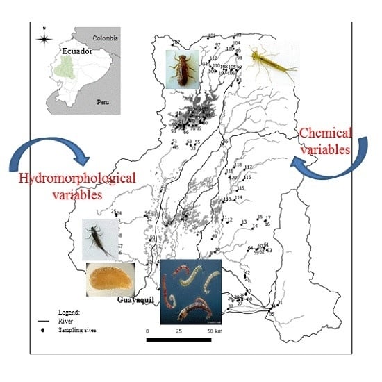
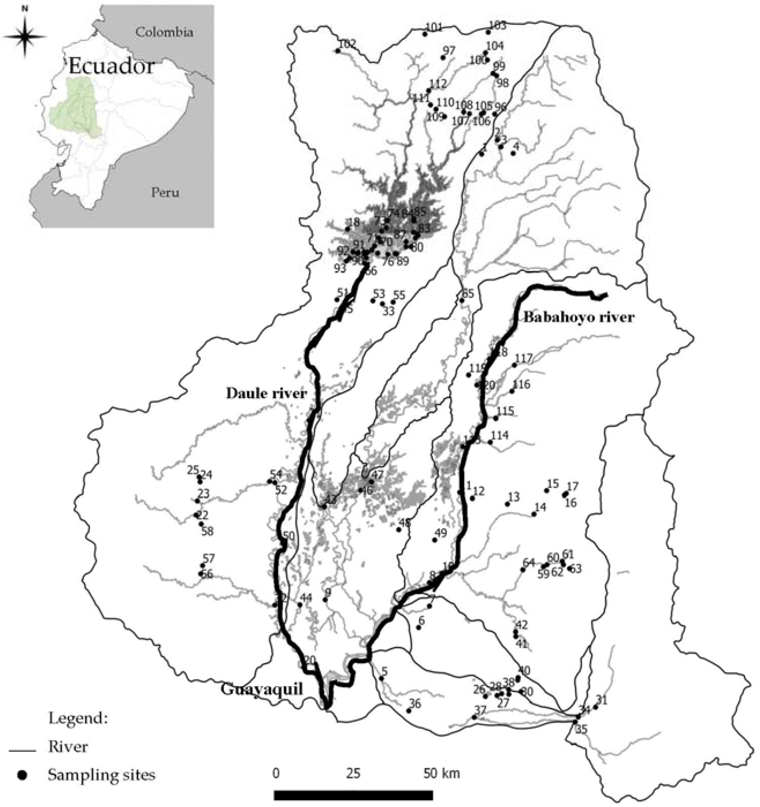
2.1. Study Area

The Guayas River basin is located in the central-western part of Ecuador, covering an area of 32,112 km2. It has an average annual precipitation of 1662 mm and discharges on average 835 m3/s into the Gulf of Guayaquil. The Daule-Peripa reservoir is located in the upstream part of the basin, and a large part of the water flowing from the upper river basin is diverted to the reservoir. The reservoir has a surface area of approximately 30,000 ha, a 6000 million-m3 water storage capacity and a 14,350-m3/s spillway natural maximum discharge. It was built for electricity generation, irrigation, flood control and drinking water supply purposes [22,23,24]. The Guayas River basin consists of two main rivers: the Daule and Babahoyo rivers.
In total, 120 sites were sampled (Figure 1). Thirty-two sampling sites were located in the Daule-Peripa reservoir, and the remaining 88 sites were situated at the up- and down-stream locations of the rivers within the Guayas River basin. The selection of sites was based on an expected gradient of disturbance from pristine (mountainous, less intensive human activities, less populated areas, clear water) to degraded (low elevation, intensive human activities, densely populated areas, colored water).

2.2. Data Collection

The sampling campaign took place from 23 October–26 November 2013, at the end of the dry season (from July–November). There was no extreme weather, such as heavy rain, during the sampling campaign, and since Ecuador is located in a tropical region, seasonal differences are not as distinct as in temperate regions [25]. Biological (macroinvertebrates) and environmental (physical-chemical and hydromorphological) variables were collected from each sampling site. Each site was sampled once as a general assessment, not to investigate point sources of pollution. In total, 39 variables were assessed (Table 1 and Table 2), and no other data were used besides the collected data. Two YSI®6920-V2 (Yellow Springs, OH, USA) multiparameter probes were used to measure temperature, conductivity, total dissolved solids (TDS), pH, chlorophyll, chloride, dissolved oxygen (DO) and turbidity; whereas chemical oxygen demand (COD), total nitrogen (total N), total phosphorus (total P), nitrate-N, nitrite-N and ammonium-N were measured in the laboratory using Hach-Lange®DR 3900 spectrophotometer kits (Loveland, CO, USA).
The measurements of COD, total N, total P, nitrate-N, nitrite-N and ammonium-N were done ex situ. Water samples were taken from each sampling site and were stored in a cool and dark container before being analyzed in the laboratory. A different treatment was performed for each variable using ready-to-use reagents and cuvettes that came together with the Hach-Lange®DR 3900 spectrophotometer kits (Loveland, CO, USA). The reading of the measurements was done using the kits’ visible (VIS) spectrophotometer with a wavelength range of 320–1100 nm and a wavelength resolution of 1 nm. Temperature, conductivity, TDS, pH, chlorophyll, chloride, DO and turbidity were measured in situ. Each probe of the two YSI®6920-V2 multiparameter probes (Yellow Springs, OH, USA) that contained different electrodes was inserted into a bucket containing a 10-L water sample. The value of each variable was noted when the reading was stable. Flow velocity was measured manually with a standard length of 5 m, using the float method, as described in the U.S. Environmental Agency [26] protocol. Stream width and water depth were also measured manually using the tape measure, while a Garmin GPSMap® (Kansas City, MO, USA) was used to measure elevation. Due to a human error, the COD of 30 sites could not be measured; whereas due to practical limitations, the width and depth of the sites located at the reservoir and at big rivers could not be measured either.
Information of the site and its surroundings was collected regarding land use, macrophytes, riparian vegetation, river banks, channel types, flow types and sediment. We used a modified field protocol based on the Australian River Assessment System (AUSRIVAS) physical assessment protocol [27] and the United Kingdom and the Isle of Man River Habitat Survey (RHS) [28] to obtain the data. In total, 21 variables were measured following different categories (Table 2).
Benthic macroinvertebrates were sampled using the standardized kick-net method as described in Gabriels et al. [29]. The net had a mesh size of 500 µm and was attached to a 0.2 × 0.3-m metal frame and a 2 m-long handle. The sampling covered a stretch of approximately 10–20 m for 5 min and covered all different habitats present at the site, such as the bed substrate, macrophytes, litter and parts of terrestrial vegetation immersed in the water. Besides the kick-net method, macroinvertebrates were also picked manually from stones and leaves to collect the highest possible richness of macroinvertebrates. For sites located at the reservoir, the macroinvertebrates were sampled at the shorelines. Whereas for sites located away from the shorelines, the macroinvertebrates were sampled from the macrophytes. Macroinvertebrates were then sorted from the samples and were identified to the family level. The identification was done based on the identification keys of De Pauw et al. [30] and Domínguez and Fernández [31]. Each family was also identified for its functional feeding group (FFG) based on Mereta et al. [32], Barbour et al. [33] and Helson and Williams [2], summarized in Table S1 with relevance to the river continuum concept [34].

2.3. Biotic Integrity

The biotic integrity of each sampling site was calculated using the Biological Monitoring Working Party (BMWP) adapted for Colombia (BMWP-Col) [35], based on Alvarez [36]. The BMWP-Col was used since Ecuador does not have its own water quality index based on macroinvertebrates. This index is considered an appropriate index for Ecuador, since Colombia has relatively similar environmental conditions to Ecuador [37]. Moreover, Dominguez-Granda et al. [37] and Damanik-Ambarita et al. [38] also used the BMWP-Col to assess the water quality in the Chaguana and Guayas river basins in Ecuador, respectively. Damanik-Ambarita et al. [38] concluded that the BMWP-Col was more suitable for the current study area, as compared to the Neotropical Low-land Stream Multimetric Index (NLSMI), a locally-developed multimetric index that incorporates seven individual metrics [2]. The BMWP-Col calculation was performed based on the macroinvertebrate community composition, wherein each macroinvertebrate taxon is associated with a certain tolerance score. The tolerance score ranged from 1 to 10 (Table S1), with low scores representing tolerant taxa and high scores representing sensitive taxa. A BMWP-Col score of more than 100 represents good biotic integrity, 61–100 represents moderate, 36–60 poor, 16–35 bad and 0–15 very bad biotic integrity [36]. Since elevation might influence macroinvertebrate community composition, it might influence the BMWP-Col calculation. Therefore, we also calculated the average score per taxon (ASPT) index to define a biotic integrity that is independent of taxonomic richness and elevation. The ASPT values were then related with the elevation and their correlation coefficient (R2) was calculated. A strong correlation would confirm the influence of elevation on biotic integrity and vice versa. The ASPT was calculated by dividing the BMWP-Col score with the number of taxa encountered per site, and it ranges from 0 to 10. An ASPT score of more than 6 indicates clean water; 5–6 indicates doubtful quality; 4–5 probable moderate pollution; and less than 4 indicates probable severe pollution [39,40]. The degree of habitat degradation was calculated, as well, using an adapted habitat disturbance score (Table S2) as described by Barbour et al. [33], Hruby [41], USEPA [42] and Mereta et al. [32].

2.4. Statistical Model

Our aim of making the model was to identify key environmental variables influencing the presence of macroinvertebrates in the Guayas River basin, Ecuador. In total, 39 variables were monitored (Table 1 and Table 2). However, chemical oxygen demand (COD), stream width and stream depth were removed before the analysis due to missing values. Furthermore, following the procedure described in Zuur [43] and Zuur et al. [44], 12 collinear variables were removed based on variance inflation factors (VIF), wherein variables with VIF values higher than three were regarded as collinear. Based on these pre-processing steps, 24 variables were included in the analysis (Table 1 and Table 2). Next, a generalized linear model (GLM) was used to determine key environmental variables influencing the biotic integrity [43,45], expressed as BMWP-Col. The GLM was selected since it has been widely used for ecological-related studies [22,46,47] and has proven its ability to study non-linear relationships, as observed in our data. The continuous variables were not transformed (e.g., log-transformation) before analysis to avoid difficult interpretation of the models afterwards, while categorical variables were set as factors. We also did not remove outliers from the analysis, since they are real observations (not technical errors) and to avoid reducing the number of observations. Besides, another advantage of choosing the GLM is because the GLM can deal with extreme values, such as outliers [44].
We have used three-fold cross-validation to train and validate the GLMs. To do so, the complete dataset was randomly split into three equal subsets. Each subset was used to validate the model, while the remaining two subsets were used for model development [48]. This means that two parts of the dataset were used for training and one part for testing. Prior to splitting, the dataset was stratified based on the BMWP-Col classes. The use of the BMWP-Col classes in stratifying the dataset was based on the study by Everaert et al. [18] who used the ecological quality ratio (EQR) status in their analysis. To assess the robustness of the three-fold cross-validation, we compared the model developed based on 2/3 of the data with a model that was developed based on the complete dataset. Hence, two sets of models were inferred: models developed from and validated on the complete dataset (120 sites) and models developed from and validated based on three-fold cross-validation (Figure S1).
Since the dependent variable (BMWP-Col) is continuous, we used a Gaussian distribution for model development. The drop1 command was used to remove variables that did not contribute to the model fit, starting from the variable with the least significant p-value. The drop1 command drops one variable each time and for the Gaussian distribution performs an F-test based on residual sum of squares of a full model [43]. The process was continued, and the Akaike information criteria (AICs) of different model configurations were compared. Since a model with a lower AIC was regarded to better fit the data, we looked for the model with the lowest AIC. However, models with the lowest AICs did not always contain all variables with p-values significant at p < 0.05. To address the situation, variable removal using the drop1 command was continued until we reached the models with all variables significant at p < 0.1 and p < 0.05, respectively. Two p-value criteria were used to see the significant difference among variables contained in models from different partitions. The stability of the results of the models was evaluated by ranking the input variables based on their presence in each model. To do this, each variable was listed according to its significance in the model (based on its p-value). The variable lists from all models were then combined to get the final ranks of the variables. All analyses were performed with R software Version 3.0.2 (25 September 2013); the drop1 command is available in R without specific packages [49].

2.5. Sensitivity Analysis: Identifying Potential Restoration Actions

The sensitivity analysis assessed the effect of an explanatory variable towards the response variable under a given situation [50,51,52]. The variables contained in the final models were selected to illustrate the effects of changing their values on the biotic integrity expressed as the BMWP-Col. To do so, other variables included in the models were assumed not to cause restrictions and set constant to their median values. One variable, the one for which we assessed its influence on the response variable (i.e., BMWP-Col), ranged between the minimum and maximum values of the monitoring data (i.e., complete dataset). The analysis was done in a similar way for both continuous and categorical variables, wherein the median, minimum and maximum values for categorical variables were based on their description (Table 2). The median categories for categorical variables were the most encountered categories. The results were then used as the basis of potential restoration actions to maintain good biotic integrity or to improve biotic integrity (based on the outcome of the BMWP-Col) by addressing the variables selected in the models.

3. Results

3.1. Bioassessment Indices and Biotic Integrity

The biotic integrity based on the BMWP-Col ranged from 0 to 168 and 0 to 7.3 for the ASPT. High values of both indices were observed at sites located at higher elevations having forested land use and mountainous areas. High indices values were also observed at tributaries of the rivers located at lower elevations (Figures S2 and S3). Generally, high BMWP-Col and ASPT values were observed at sites with a low concentration of chlorophyll, nitrate-N and nitrite-N. High BMWP-Col values were also witnessed at sites where DO concentrations ranged from 6 to 10 mg/L, turbidity was lower than 20 Nephelometric Turbidity Units and flow velocity was higher than or equal to 0.2 m/s. A 90% of shading, a sludge layer of less than 5 cm and the presence of dead wood in the rivers were related to a high BMWP-Col and ASPT (Figure 2 and Figure S4). Hence, both indices indicated similar environmental conditions, as can be seen from their positive correlation (Figure S5). Figures S2 and S3 indicated the elevation division of higher and lower than 250 m; therefore, we plotted the FFG separately for sites located at elevation higher and lower than 250 m, as well as for the reservoir (Figure S6). Collectors were dominant at both higher and lower than a 250-m elevation (mean percentage 60.3% and 40.2%, respectively), while predators and collectors dominated the sites at the reservoir (mean percentage 45% and 33%, respectively). The habitat disturbance score ranged from 11 to 26 (Figure S7), where high index scores were found in both undisturbed (indicated by high habitat disturbance scores) and disturbed (indicated by low habitat disturbance scores) habitats. Despite the ASPT classification of poor scores indicating pollution, our data showed the possible cause of habitat alteration, as well.

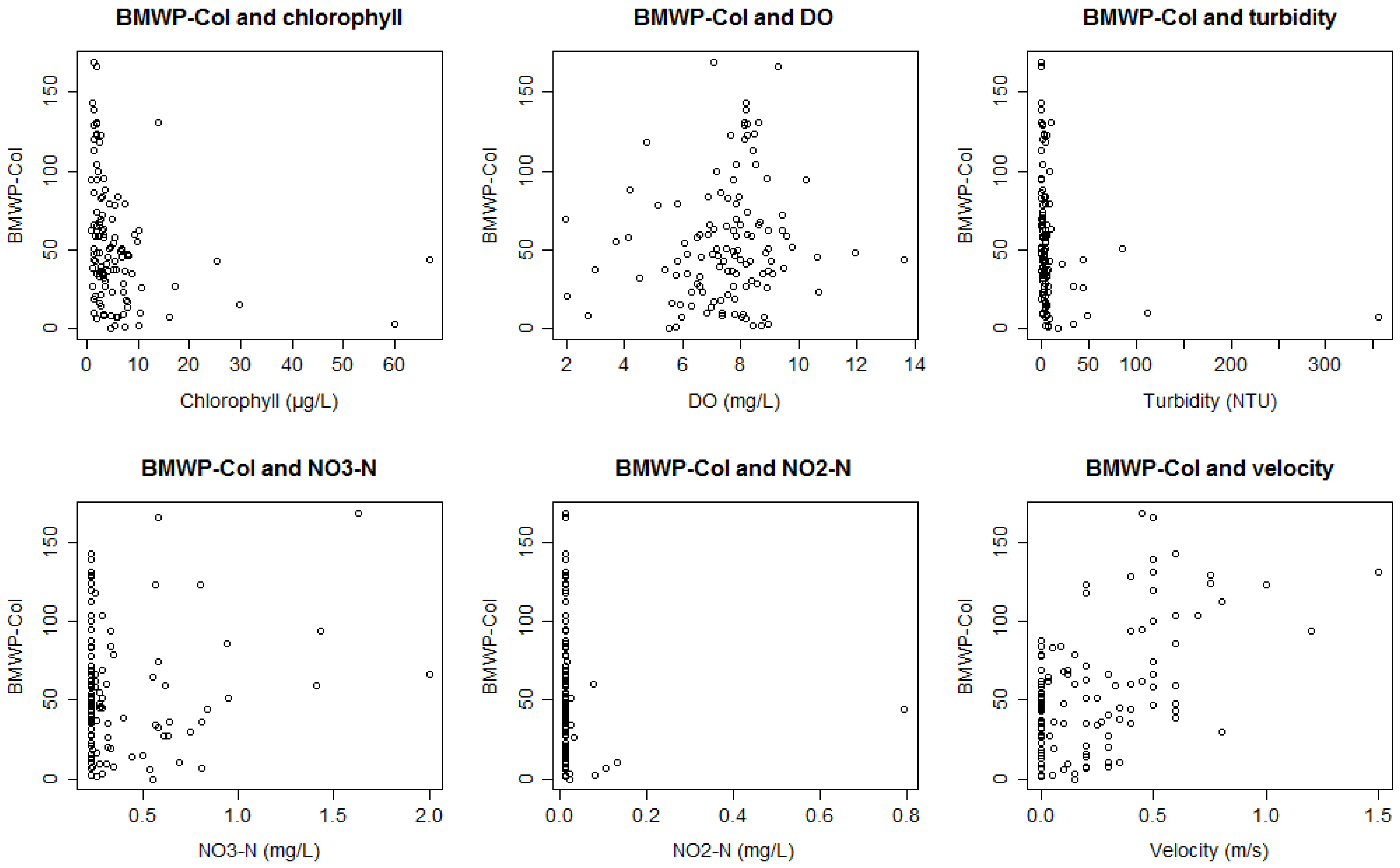
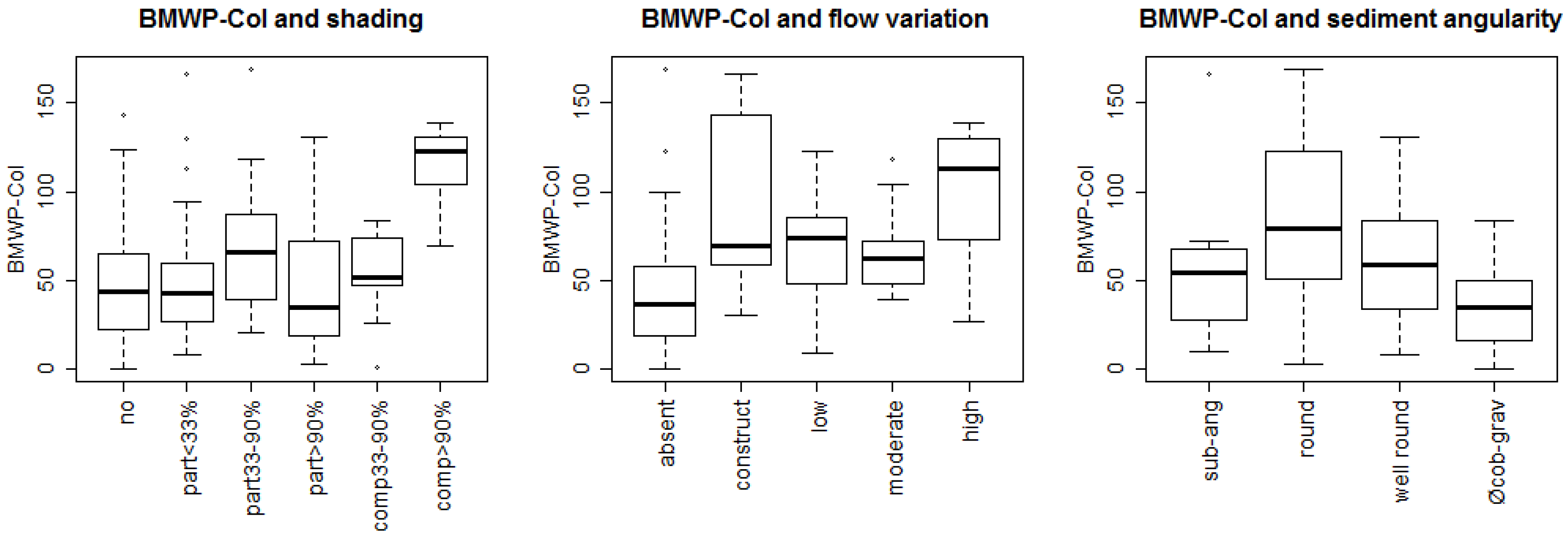
3.2. Statistical Model

We found that physical-hydromorphological (i.e., elevation, sediment angularity, logs, main macrophytes, flow velocity, turbidity, bank shape and land use) and chemical (i.e., nitrate-N and chlorophyll concentration) variables are the main drivers of the biotic integrity expressed as the BMWP-Col. In total, 16 variables were selected based on the three-fold cross-validation (i.e., nitrate-N, chlorophyll, turbidity, flow velocity, elevation, sediment angularity, valley form, twigs, branches, logs, land use, bank slope, bank shape, main macrophytes, erosion and variation in flow). However, different data partitions from the three-fold cross-validation resulted in varied selected variables and significant levels.
Elevation was the most significant variable, while nitrate-N was the only nutrient variable that came up in each criterion. For Training Set 1 + 2, 11 variables were selected based on the model with the lowest AIC: elevation, main macrophytes, nitrate-N, sediment angularity, logs, land use, erosion, chlorophyll, flow variation, velocity and bank slope, with p-values of 0.001, 0.013, 0.024, 0.027, 0.044, 0.048, 0.048, 0.064, 0.067, 0.151 and 0.181, respectively. The variables’ selection is presented in Table S3, while the final models are shown in Table S4 together with their ranks. Fold 1 (Training Set 1 + 2 and Testing Set 3) had the highest R2 value for testing set compared to other folds. The R2 values were 0.57 and 0.49 for Training Set 1 + 2 and Testing Set 3, respectively. Compared to other criteria, the model with the lowest AIC gave the highest R2 value (Table S5). The results of other data partitions are presented in the Supporting Information (Tables S3–S5). Residual plots and model validation are presented in the Supporting Information (Figures S8–S23). For the model based on the complete dataset, 10 variables were selected that corroborated the results of the three-fold cross-validation (Tables S6 and S7 and Figures S24–S32).

3.3. Sensitivity Analysis

Besides elevation, all other variables in the models were also investigated in the sensitivity analysis to assess their effects on the BMWP-Col values (Table S8). Here, we present the impacts of changing the elevation, nitrate-N concentration, sediment angularity and logs (Figure 3). The sensitivity analysis of elevation clearly showed that the BMWP-Col increased from 35 (bad)–122 (good) if the elevation is increased from 2 to 1080 m. Our data showed that a nitrate-N concentration higher than 0.6 mg/L was associated with poor biotic integrity, whereas the sensitivity analysis suggested an improvement in biotic integrity from 39 (poor) to 118 (good) for nitrate-N concentrations between 0 and 2.1 mg/L. Due to this finding, we further checked the relationship between the nitrate-N and other variables that might be related to nitrate-N, i.e., chlorophyll and dominant macrophytes. Several sites with nitrate-N concentrations higher than 0.5 mg/L were found where chlorophyll concentrations were lower than 10 µg/L. Nitrate-N concentrations higher than 0.5 mg/L were also detected at sites where macrophytes were absent or where floating macrophytes were present (Figure S33). More angular sediment (sub-angular and round types) could promote the biotic integrity, and a similar improvement is suggested by having abundant logs in the rivers.
The figures of other variables are given in the Supplementary Materials (Figures S34 and S35), namely dominant macrophytes, velocity, turbidity, bank shape, land use and chlorophyll. The sensitivity analysis of dominant macrophytes suggested that the BMWP-Col will increase from 1 to 82 when floating macrophytes are introduced into macrophyte-free rivers (Figure S34). Similarly, by increasing the flow velocity from 0 to 1.5 m/s the BMWP-Col will increase from 34 (bad) to 88 (moderate). A turbidity of higher than 79 Nephelometric Turbidity Units will negatively affect the BMWP-Col, whereas a change in the river bank will improve the BMWP-Col. Moreover, by changing the land use from residential to arable, the BMWP-Col will increase from 0 (very bad) to 45 (poor), and a decrease in chlorophyll concentration will promote the biotic integrity (Figure S35). The given figures are chosen from the model with the lowest AIC where the variable had the most significant p-value; for example, nitrate had the lowest p-value in the model resulting from Training Set 2 + 3.

4. Discussion

4.1. Biotic Integrity and Potential Restoration Actions

Elevation, nitrate-N concentration, sediment angularity, logs, main macrophytes, flow velocity, turbidity, bank shape, land use and chlorophyll concentration were the major variables that influenced the biotic integrity expressed as the BMWP-Col in the Guayas River basin. For management purposes, ensuring proper land use at different altitudes and monitoring the concentrations of nutrients that enter the surface waters can address most of the aforementioned variables.
Elevation was present in all models and, thus, is an important variable explaining the observed biotic integrity of the river basin. The importance of elevation in determining the water quality has often been reported [14,53,54]. However, its impacts often depend on several physical and chemical variables that are correlated with the altitude, such as temperature and oxygen levels, the type of substrates (coarser sediment is present more at a higher elevation), flow velocity and the level of disturbance related to land use and waste water discharges, due to less intensive human activities at higher elevation. For example, Malmqvist and Maki [53] related the importance of elevation with temperature, while Rezende et al. [14] linked elevation with the richness and density of macroinvertebrates. Younes-Baraille et al. [54] found a correlation between the elevation and more intensive human activities along the Andorran rivers. Intensification of human settlements at the lower elevation in Andorra increases the organic and nutrients load into the water that consequently decreases the water quality [54].
The elevation also influences the presence of macroinvertebrates. The river continuum concept (RCC) suggested that upstream rivers are generally characterized by the presence of shredders due to the rich presence of coarse particulate organic matter (CPOM) in the water, while downstream rivers are generally characterized by collectors that take advantage of fine particulate organic matter (FPOM) [34]. Our data showed the dominance of collectors at higher and lower elevations and low presence of shredders at higher elevations, as opposed to the RCC for higher elevations [38]. The RCC was observed at the reservoir, where predators and collectors were dominant. The land use surrounding the sites and the type of sediments might influence the presence of FFG [55,56,57,58], and the dry season might not provide enough CPOM upstream for the shredders to survive. The increased temperature during the dry season might also negatively influence certain taxa [34].
Although one cannot alter elevation, the land use can be managed adequately at different altitudes. Previous studies have shown the impacts of land use on the water quality, in relation to the elevation. Different land uses at different altitudes are present in our study area, which means that different management actions are needed. At higher elevations, preserving forest in mountainous areas is necessary to maintain a low conductivity, low temperature, low turbidity, low TDS and high DO concentration of the water [59]. Forest also provides food for macroinvertebrates, through its leaf and wood litter [60], prevents nonpoint-source pollutants from entering the streams, and enhances in-stream processing of pollutants [61]. Revegetation of riparian areas can decrease the TDS concentration of the water, and its canopy cover also reduces water temperature [62]. Since agricultural activities are more likely to occur in flatter landscapes [63], its proper management is needed to preserve water quality. Ellison et al. [62] argued that reducing animal grazing in riparian zones is a necessary management option, especially during the summer/dry season, because grazing animals might degrade river banks, lower the water table, and increase water turbidity. Moreover, proper regulation and management of agrochemical use are crucial to reduce the impacts on water quality and macroinvertebrates [63]. Other options to improve the water quality are providing more sanitary infrastructures [64] and installing a wastewater treatment plant [54] to treat urban wastewater. Nevertheless, we suggest the exclusion of elevation from future studies to analyze environmental impacts on the biotic integrity that is independent of elevation.
A second factor that influenced the biotic integrity was the concentration of nitrate-N in the surface water. Generally, a nitrate-N concentration higher than 5 mg/L in surface waters indicates pollution, and concentrations higher than 0.2 mg/L may stimulate algal growth and indicate eutrophic conditions in lakes [65]. Our data confirm this principle, while the sensitivity analysis suggested an improvement in biotic integrity with increasing nitrate-N concentration. Since aquatic plants require nitrogen compounds as their nutrient source [66], perhaps our results explain this relationship. Plus with regard to general conditions, there is the possibility of a turning point in the sensitivity analysis when the nitrate-N concentration has reached a certain tipping point, which we did not study. The presence of nutrients, especially nitrate and phosphate, can also promote the concentration of chlorophyll in surface waters. High concentrations of chlorophyll can indicate pollution, in particular eutrophication [65]. However, our data did not show a positive relationship between nitrate-N and chlorophyll. Garcia et al. [67] suggested that the increase in chlorophyll concentration is highly influenced by long exposure of the surface water to sunlight and rapid uptake of nutrients by primary producers, thus explaining the high chlorophyll concentration, but low nitrate-N concentration; whereas a positive relationship between nitrate-N and macrophytes was observed at several sites, especially at sites with the presence of floating macrophytes. Chapman [65] has discussed the role of nutrients in the development of macrophytes, and Arimoro et al. [3] argued the importance of macrophytes presence in the rivers to provide a suitable microhabitat for certain macroinvertebrates, such as dipterans and odonatas, which was the case in the current study. Thus, macrophyte presence can improve the biotic integrity. Moreover, Nguyen et al. [22] has confirmed a positive correlation between water hyacinth (floating macrophytes) and macroinvertebrate’s diversity and the water quality. O’Toole et al. [68] suggested an association between mesotrophic waters and most macroinvertebrate taxa, whereas plecopterans are more associated with oligotrophic and chironomids and tubificids are tolerant with eutrophic waters. Furthermore, the concentration of nitrate-N in our study was generally low, even below the guidelines for surface waters from the Ministerio del Ambiente del Ecuador (MAE, 13 mg/L) and the European Commission (EC, 50 mg/L) [69,70]. Our observed maximum concentration of nitrate-N also equaled the appropriate maximum level to protect the most sensitive freshwater species (2 mg/L) [71,72]. A previous study by Borbor-Cordova et al. [73] suggested that some parts of the Guayas River basin have experienced nutrient loss and soil degradation due to their intensive farming activities, in which the amount of nutrients that leave the soil through exported crops is higher than the original soil content plus the applied chemical fertilizers [73]. This finding suggests another possible explanation that the Guayas River basin might require a certain amount of nitrate-N for its productivity. Nevertheless, future management of biotic integrity needs to keep the concentration of nitrate-N lower than the guidelines.
We also found that angular sediment promotes the biotic integrity, since more angular sediment allows macroinvertebrates to attach onto the sediment surface and avoid their drifting [74]. The angularity or roundness of sediment indicates the amount of transport it had, and fine sediment deposition in the water can reduce the angularity of the rock [75]. Regarding bank shape, several studies suggested the importance of stable river banks to improve the water quality and the macroinvertebrate community. Raymond and Vondracek [76], for example, suggested a positive correlation between a stable river bank and the macroinvertebrate assemblage by converting conventional grazing to rotational grazing in farming. Similar to land use management, Lester and Boulton [77] also suggested that bank stability can be improved through the exclusion of grazing animals from river banks and revegetation of the river banks.
Another key variable was the flow velocity, which is often highly diverse in a river basin. Flow velocity is generally related to the elevation [20], the amount of rainfall and water transport through the basin. Flow velocity is also linked with the substrate, land use and channel slopes in the up-stream locations [60]. The importance of velocity in studying water quality was also deduced by Hughes et al. [9] and Arimoro et al. [3]. A slow flow velocity allows the deposition of fine sediments [78,79], which consequently inhibits water exchange and oxygen transport [80] and supports nutrients and contaminants transfer [81] within the water, a condition that can be harmful to aquatic animals. A high flow velocity provides more suitable habitat and offers continuous food and oxygen supply for aquatic animals, thus improving the biotic integrity [37,82,83]. However, altering the flow velocity of the rivers is difficult, especially in low-land areas, where flow increase can only be induced by a lower water use (e.g., irrigation) or the removal of obstructions at the upstream, such as hydropower dams.
At the downstream parts of the rivers and at tributaries that were disconnected from their main channels, we observed elevated levels of several environmental variables, such as conductivity. We assume that this is related to the seasonality, where the late dry season is usually characterized by the lower water quality conditions of the surface waters, since environmental variables have reached their extreme levels. Generally, temperature, conductivity, chlorophyll and turbidity highly increase through the dry season [8,10,67]. The temperature, pH, conductivity, turbidity and DO vary temporally, and more specifically, the temperature follows seasonal trajectories, while DO can vary significantly within a 12-h period at similar depths [8]. Low nutrient levels, but increasing chlorophyll and primary production through the dry season indicate rapid nutrient uptake by primary producers due to long exposures to sunlight [67]. Increasing disturbance also influences the presence of more tolerant macroinvertebrates, and the interruption from upstream assemblages during the dry season reduces macroinvertebrates abundance and diversity. However, macroinvertebrates’ responses towards environmental changes might vary spatially and across habitats [2,8,38,67]. The dry season is also characterized by low flow periods, whereas high flooding flows characterize the wet season. During the wet season, wet season floods support ecosystem replenishment, and habitat conditions are getting more stable when floods recede, which then allows the settlement and growth of macroinvertebrate communities [38,67]. However, we could not compare the conditions during dry and wet seasons, since the sampling campaign was only performed at the end of the dry season. Moreover, Greenwood and Booker [84] stressed the importance of studying the temporal variations of hydrological and ecological data to capture the full picture of aquatic systems and to define the response of aquatic organisms towards disturbances. Because our sampling campaign was only performed once and within a short period, we also could not assess the degree of hydrological and ecological variability of the rivers over time, as well as the variations in community compositions. Thus, continuous monitoring of the aforementioned variables during dry and wet seasons can provide better understanding of the temporal variations of the biotic integrity of the river basin.

4.2. Model Development and Validation

Dealing with a complex and dynamic system in aquatic ecology, the correlation coefficient R2 values of all models, both models using the complete dataset and those using three-fold cross-validation, indicated a good model fitness to predict the biotic integrity. We tested the robustness of the outcome of the modelling exercises and found that models based on the complete dataset had similar R2 values for development and validation. However, when assessing each of the separate folds, we observed that the R2 values of the training datasets ranged from 0.52 to 0.62, and the validation datasets ranged from 0.31 to 0.49. However, certain variables were always selected as key variables, despite their relative p-values. As such, the use of cross-validation is helpful to avoid the model overfitting. Cross-validation also allows model validation using an independent dataset without reducing the number of samples that can be used [43]. Thus, this shows the importance of the variable’s ranking in defining the most influencing variables from all key variables, instead of choosing one best model. This way, more options are available for monitoring and restoration actions. However, we recommend the use of the lowest AIC to select the best model in future studies.
The parameter used to stratify the dataset before splitting was assumed to be the cause for the presence of several ‘outliers’ in the residual plots of the models. Most of them represented the same sites with very high BMWP-Col values within the dataset. The models under-predicted the biotic integrity values as compared to the actual values, while the remaining few other sites were overly predicted. These results suggested that the models can predict the biotic integrity within a certain range of values. To improve model performance, we recommend that future studies can be done by splitting the dataset based on the BMWP-Col values, instead of its classes. We also recommend to analyze the reservoir, up- and down-stream parts of the river basin separately.
Our results proved the ability of GLMs to determine the relative importance of each environmental variable towards the biotic integrity and macroinvertebrate communities in particular, which is an advantage over other techniques, such as ANN [47,52]. However, we also experienced one limitation of using GLMs as compared to other techniques. The GLM is unable to deal with missing data, whereas Bayesian belief networks (BBN) can easily deal with this issue [20]; thus, we needed to remove variables with missing values (i.e., COD, stream width and stream depth) before starting the model selection process [43]. Nevertheless, recommending the use of one particular model for a given problem is practically impossible, and each study may require a different modelling technique [85].

5. Conclusions

We found that the physical-hydromorphological (i.e., elevation, sediment angularity, logs, main macrophytes, flow velocity, turbidity, bank shape and land use) and chemical (i.e., nitrate-N and chlorophyll concentrations) variables were the major variables that influenced the macroinvertebrates of the Guayas River basin in Ecuador. We analyzed the relevance of the variables via a sensitivity analysis, and cross-fold validation provided insights for the stability of the outcomes. To restore and protect river ecosystems and their functions, and in particular, macroinvertebrate communities, policy actions need to focus on alterable variables, such as the land use at different elevations, management and monitoring of nitrate-N and chlorophyll concentrations, macrophyte presence, sediment transport and bank stability.

Supplementary Materials

The following are available online at www.mdpi.com/2073-4441/8/7/297/s1. Figure S1: Scheme for the model development and criteria for the final models, Figure S2: The biotic integrity expressed as the BMWP-Col of sites at different elevations, Figure S3: The biotic integrity expressed as the ASPT of sites at different elevations, Figure S4: Relationship between environmental variables and the biotic integrity expressed as ASPT, classification of categorical variables are based on Table 2; compos: composite, nat: natural, art: artificial, constr: construction, var: variation, part: partly, comp: completely, ang: angular, cob-grav: cobble-pebble-gravel, Figure S5: Correlation between BMWP-Col and ASPT and its correlation coefficient, Figure S6: Percentage of the functional feeding group (FFG) that comprises the percentage of scrapers, shredders, collector-gatherer, collector-filterer and predator encountered at the sampling sites: for 120 sampling sites (A); for sites located at the elevation lower than 250 m (B); for sites located at the elevation higher than 250 m (C); and for sites located at the reservoir (D), Figure S7: Habitat disturbance score in relation with BMWP-Col (a) and ASPT (b), Figure S8: Residuals’ plots of the model based on the folds’ Training Set 1 + 2 with the lowest AIC, (a) residuals versus fitted values; (b) QQ-plot for normality; (c) scaled residuals versus fitted values; (d) standardized residuals versus leverage, Figure S9: Validation of the model based on the folds’ Test Set 3 with the lowest AIC, Figure S10: Residuals’ plots of the model based on the folds’ Training Set 1 + 2 with input variables significant at p < 0.1, (a) residuals versus fitted values; (b) QQ-plot for normality; (c) scaled residuals versus fitted values; (d) standardized residuals versus leverage, Figure S11: Validation of the model based on the folds’ Test Set 3 with input variables significant at p < 0.1, Figure S12: Residuals’ plots of the model based on the folds’ Training Set 1 + 2 with input variables significant at p < 0.05, (a) residuals versus fitted values; (b) QQ-plot for normality; (c) scaled residuals versus fitted values; (d) standardized residuals versus leverage, Figure S13: Validation of the model based on the folds’ Test Set 3 with input variables significant at p < 0.05, Figure S14: Residuals’ plots of the model based on the folds’ Training Set 1 + 3 with the lowest AIC, (a) residuals versus fitted values; (b) QQ-plot for normality; (c) scaled residuals versus fitted values; (d) standardized residuals versus leverage, Figure S15: Validation of the model based on the folds’ Test Set 2 with the lowest AIC, Figure S16: Residuals’ plots of the model based on the folds’ Training Set 1 + 3 with input variables significant at p < 0.1, (a) residuals versus fitted values; (b) QQ-plot for normality; (c) scaled residuals versus fitted values; (d) standardized residuals versus leverage, Figure S17: Validation of the model based on the folds’ Test Set 2 with input variables significant at p < 0.1, Figure S18: Residuals’ plots of the model based on the folds’ Training Set 1 + 3 with input variables significant at p < 0.05, (a) residuals versus fitted values; (b) QQ-plot for normality; (c) scaled residuals versus fitted values; (d) standardized residuals versus leverage, Figure S19: Validation of the model based on the folds’ Test Set 2 with input variables significant at p < 0.05, Figure S20: Residuals’ plots of the model based on the folds’ Training Set 2 + 3 with the lowest AIC and input variables significant at p < 0.1, (a) residuals versus fitted values; (b) QQ-plot for normality; (c) scaled residuals versus fitted values; (d) standardized residuals versus leverage, Figure S21: Validation of the model based on the folds’ Test Set 1 with the lowest AIC and input variables significant at p < 0.1, Figure S22: Residuals’ plots of the model based on the folds’ Training Set 2 + 3 with input variables significant at p < 0.05, (a) residuals versus fitted values; (b) QQ-plot for normality; (c) scaled residuals versus fitted values; (d) standardized residuals versus leverage, Figure S23: Validation of the model based on the folds’ Test Set 1 with input variables significant at p < 0.05, Figure S24: Residuals’ plots of the model with the complete dataset and the lowest AIC, (a) residuals versus fitted values; (b) QQ-plot for normality; (c) scaled residuals versus fitted values; (d) standardized residuals versus leverage, Figure S25: Validation of the model with the complete dataset and the lowest AIC, Figure S26: Validation of the model with the complete dataset and the lowest AIC on three folds, (a) for test set 1; (b) for test set 2; (c) for test set 3, Figure S27: Residuals’ plots of the model with the complete dataset and input variables significant at p < 0.1, (a) residuals versus fitted values; (b) QQ-plot for normality; (c) scaled residuals versus fitted values; (d) standardized residuals versus leverage, Figure S28: Validation of the model with the complete dataset and the input variables significant at p < 0.1, Figure S29: Validation of the model with the complete dataset and the input variables significant at p < 0.1 on three folds, (a) for test set 1; (b) for test set 2; (c) for test set 3, Figure S30: Residuals’ plots of the model with the complete dataset and the input variables significant at p < 0.05, (a) residuals versus fitted values; (b) QQ-plot for normality; (c) scaled residuals versus fitted values; (d) standardized residuals versus leverage, Figure S31: Validation of the model with the complete dataset and the input variables significant at p < 0.05, Figure S32: Validation of the model with the complete dataset and the input variables significant at p < 0.05 on three folds, (a) for test set 1; (b) for test set 2; (c) for test set 3, Figure S33: Relationship between nitrate-N and chlorophyll (a) and between nitrate-N and dominant macrophytes (b), Figure S34: The impact of changing the presence of the main macrophytes (a), velocity (b), turbidity (c) and bank shape (d) on the biotic integrity expressed as BMWP-Col, p-values of 0.013, 0.015, 0.05 and 0.036, respectively. The values used in the analysis were based on Table S8, showing the median, minimum and maximum values for sensitivity analysis, Figure S35: The impact of changing the land use (a) and chlorophyll concentration (b) on the biotic integrity expressed as BMWP-Col, p-values of 0.048 and 0.064, respectively. The values used in the analysis were based on Table S8, showing the median, minimum and maximum values for the sensitivity analysis, Table S1: List of families encountered in the Guayas River basin with tolerance scores based on Alvarez, 2005; the number present in the samples and the functional feeding group (FFG), Table S2: Adapted habitat disturbance criteria and scoring list, Table S3: Variables’ selection for three folds: showing variable with the highest p-value in the model together with the AIC of each model, Table S4: Ranking of the importance of input variables in the models with 3-fold cross-validation, based on the p-values (the p-values are given between brackets), Table S5: Predictive performances of the models with 3-fold cross-validation: showing the number of input variables that construct the models and the correlation coefficient (R2) values of training and testing sets, Table S6: Variables’ selection for the model with the complete dataset: showing the variable with the highest p-value in the model and the AIC of each model, Table S7: Variables’ ranking of importance based on the p-values for the models with the complete dataset; the p-values are given between brackets, Table S8: Median, minimum and maximum values for the sensitivity analysis of the models based on the complete dataset.

Acknowledgments

This research was performed in the context of the VLIR Ecuador Biodiversity Network project. This project was funded by the Vlaamse Interuniversitaire Raad-Universitaire Ontwikkelingssamenwerking (VLIR-UOS), which supports partnerships between universities and university colleges in Flanders and the South. The authors would also like to thank the assistance of the Department of Chemical and Environmental Sciences (Centro del Agua y Desarrollo Sustentable, Escuela Superior Politécnica del Litoral CADS-ESPOL) staff during the sampling campaign in Ecuador, Christine Van der Heyden (Hogeschool Gent) for sharing her expertise on chemical analysis of water samples. Marie Anne Eurie Forio and Minar Naomi Damanik-Ambarita are supported by the special research fund of Ghent University. Thi Hanh Tien Nguyen is funded via a Ph.D. scholarship of BTC (Belgian Technical Cooperation). Gert Everaert is supported by a post-doctoral fellowship from the Special Research Fund of Ghent University (BOF15/PDO/061) in Belgium.

Author Contributions

Minar Naomi Damanik-Ambarita was involved in sampling preparation, performed the sampling, analyzed the data and wrote the paper. Minar Naomi Damanik-Ambarita, Marie Anne Eurie Forio, Thi Hanh Tien Nguyen, Koen Lock, Peace Liz Sasha Musonge, Natalija Suhareva and Luis Dominguez-Granda prepared and performed the sampling campaign. Elina Bennetsen supported the sampling preparation. Gert Everaert, Marie Anne Eurie Forio, Pieter Boets and Peter L.M. Goethals were involved in sampling preparation, data analysis and writing the paper.

Conflicts of Interest

The authors declare no conflict of interest.

Abbreviations

The following abbreviations are used in this manuscript:
BMWPBiological Monitoring Working Party
BMWP-ColBiological Monitoring Working Party adapted for Colombia
IMEERAÍndice Multimétrico del Estado Ecológico para Ríos Altoandinos
ABIAndean Biotic Index
NLSMINeotropical Low-land Stream Multimetric Index
ASPTaverage score per taxon
GLMgeneralized linear model
ANNartificial neural networks
BBNBayesian belief networks
TDStotal dissolved solids
DOdissolved oxygen
CODchemical oxygen demand
Total Ntotal nitrogen
Total Ptotal phosphorus
Std devstandard deviation
AUSRIVASAustralian River Assessment System
RHSthe United Kingdom and the Isle of Man River Habitat Survey
FFGfunctional feeding group
VIFvariance inflation factor
EQRecological quality ratio
AICAkaike information criterion
RCCriver continuum concept
CPOMcoarse particulate organic matter
FPOMfine particulate organic matter
MAEMinisterio del Ambiente del Ecuador

References

  1. Goethals, P.L.M. Sustainability of water quality and ecology: Easier said than defined and implemented. Sustain. Water Qual. Ecol. 2013, 1, 1–2. [Google Scholar] [CrossRef]
  2. Helson, J.E.; Williams, D.D. Development of a macroinvertebrate multimetric index for the assessment of low-land streams in the neotropics. Ecol. Indic. 2013, 29, 167–178. [Google Scholar] [CrossRef]
  3. Arimoro, F.O.; Odume, O.N.; Uhunoma, S.I.; Edegbene, A.O. Anthropogenic impact on water chemistry and benthic macroinvertebrate associated changes in a southern Nigeria stream. Environ. Monit. Assess. 2015, 187, 1–14. [Google Scholar] [CrossRef] [PubMed]
  4. Bruno, D.; Belmar, O.; Sanchez-Fernandez, D.; Guareschi, S.; Millan, A.; Velasco, J. Responses of Mediterranean aquatic and riparian communities to human pressures at different spatial scales. Ecol. Indic. 2014, 45, 456–464. [Google Scholar] [CrossRef]
  5. Frankforter, J.D.; Weyers, H.S.; Bales, J.D.; Moran, P.W.; Calhoun, D.L. The relative influence of nutrients and habitat on stream metabolism in agricultural streams. Environ. Monit. Assess. 2010, 168, 461–479. [Google Scholar] [CrossRef] [PubMed]
  6. Silva, D.M.L.; Camargo, P.B.; Mcdowell, W.H.; Vieira, I.; Salomao, M.S.M.B.; Martinelli, L.A. Influence of land use changes on water chemistry in streams in the State of Sao Paulo, southeast Brazil. An. Acad. Bras. Cienc. 2012, 84, 919–930. [Google Scholar] [CrossRef] [PubMed]
  7. Karr, J.R. Biological Integrity—A Long-Neglected Aspect of Water-Resource Management. Ecol. Appl. 1991, 1, 66–84. [Google Scholar] [CrossRef]
  8. Blanchette, M.L.; Pearson, R.G. Dynamics of habitats and macroinvertebrate assemblages in rivers of the Australian dry tropics. Freshw. Biol. 2013, 58, 742–757. [Google Scholar] [CrossRef]
  9. Hughes, S.J.; Santos, J.M.; Ferreira, M.T.; Caraca, R.; Mendes, A.M. Ecological assessment of an intermittent Mediterranean river using community structure and function: Evaluating the role of different organism groups. Freshw. Biol. 2009, 54, 2383–2400. [Google Scholar] [CrossRef]
  10. Everaert, G.; De Neve, J.; Boets, P.; Dominguez-Granda, L.; Mereta, S.T.; Ambelu, A.; Hoang, T.H.; Goethals, P.L.M.; Thas, O. Comparison of the Abiotic Preferences of Macroinvertebrates in Tropical River Basins. PLoS ONE 2014, 9, e108898. [Google Scholar] [CrossRef] [PubMed]
  11. Dudgeon, D.; Arthington, A.H.; Gessner, M.O.; Kawabata, Z.I.; Knowler, D.J.; Leveque, C.; Naiman, R.J.; Prieur-Richard, A.H.; Soto, D.; Stiassny, M.L.J.; et al. Freshwater biodiversity: Importance, threats, status and conservation challenges. Biol. Rev. 2006, 81, 163–182. [Google Scholar] [CrossRef] [PubMed]
  12. Alvarez-Mieles, G.; Irvine, K.; Griensven, A.V.; Arias-Hidalgo, M.; Torres, A.; Mynett, A.E. Relationships between aquatic biotic communities and water quality in a tropical river-wetland system (Ecuador). Environ. Sci. Policy 2013, 34, 115–127. [Google Scholar] [CrossRef]
  13. Knee, K.L.; Encalada, A.C. Land Use and Water Quality in a Rural Cloud Forest Region (Intag, Ecuador). River Res. Appl. 2014, 30, 385–401. [Google Scholar] [CrossRef]
  14. Rezende, R.S.; Santos, A.M.; Henke-Oliveira, C.; Goncalves, J.F. Effects of spatial and environmental factors on benthic a macroinvertebrate community. Zoologia 2014, 31, 426–434. [Google Scholar] [CrossRef]
  15. Villamarin, C.; Rieradevall, M.; Paul, M.J.; Barbour, M.T.; Prat, N. A tool to assess the ecological condition of tropical high Andean streams in Ecuador and Peru: The IMEERA index. Ecol. Indic. 2013, 29, 79–92. [Google Scholar] [CrossRef]
  16. Rios-Touma, B.; Encalada, A.C.; Fornells, N.P. Macroinvertebrate Assemblages of an Andean High-Altitude Tropical Stream: The Importance of Season and Flow. Int. Rev. Hydrobiol. 2011, 96, 667–685. [Google Scholar] [CrossRef]
  17. Arias-Hidalgo, M.; Villa-Cox, G.; Griensven, A.V.; Solorzano, G.; Villa-Cox, R.; Mynett, A.E.; Debels, P. A decision framework for wetland management in a river basin context: The “Abras de Mantequilla” case study in the Guayas River Basin, Ecuador. Environ. Sci. Policy 2013, 34, 103–114. [Google Scholar] [CrossRef]
  18. Everaert, G.; Pauwels, I.S.; Boets, P.; Verduin, E.; de la Haye, M.A.A.; Blom, C.; Goethals, P.L.M. Model-based evaluation of ecological bank design and management in the scope of the European Water Framework Directive. Ecol. Eng. 2013, 53, 144–152. [Google Scholar] [CrossRef]
  19. Hoang, T.H.; Lock, K.; Mouton, A.; Goethals, P.L.M. Application of classification trees and support vector machines to model the presence of macroinvertebrates in rivers in Vietnam. Ecol. Inform. 2010, 5, 140–146. [Google Scholar] [CrossRef]
  20. Forio, M.A.E.; Landuyt, D.; Bennetsen, E.; Lock, K.; Nguyen, T.H.T.; Damanik-Ambarita, M.N.; Musonge, P.L.S.; Boets, P.; Everaert, G.; Dominguez-Granda, L.; et al. Bayesian belief network models to analyse and predict ecological water quality in rivers. Ecol. Model. 2015, 312, 222–238. [Google Scholar] [CrossRef]
  21. Arriaga, L. The Daule-Peripe dam project, urban development of Guayaquil and their impact on shrimp mariculture. In A Sustainable Shrimp Mariculture Industry for Ecuador; Olsen, S., Arriaga, L., Eds.; Coastal Resources Center, University of Rhode Island: Narragansett, RI, USA, 1989. [Google Scholar]
  22. Nguyen, T.H.T.; Boets, P.; Lock, K.; Damanik-Ambarita, M.N.; Forio, M.A.E.; Sasha, P.; Dominguez-Granda, L.E.; Hoang, T.H.T.; Everaert, G.; Goethals, P.L.M. Habitat suitability of the invasive water hyacinth and its relation to water quality and macroinvertebrate diversity in a tropical reservoir. Limnologica 2015, 52, 67–74. [Google Scholar] [CrossRef]
  23. United States Army Corps of Engineers (USACE). Water Resources Assessment of Ecuador; USACE: Mobile, AL, USA, 1998. [Google Scholar]
  24. Corporación Eléctrica del Ecuador (CELEC). Revista 25 Años de la Presa Daule-Peripa; CELEC: Cuenca, Ecuador, 2013. [Google Scholar]
  25. Kang, S.M.; Seager, R.; Frierson, D.M.W.; Liu, X.J. Croll revisited: Why is the northern hemisphere warmer than the southern hemisphere? Clim. Dyn. 2015, 44, 1457–1472. [Google Scholar] [CrossRef]
  26. United States Environmental Protection Agency (USEPA). Stream flow. In Water: Monitoring & Assessment; USEPA: Washington, DC, USA, 2012. [Google Scholar]
  27. Parsons, M.; Thoms, M.; Norris, R. Australian River Assessment System: AusRivAS Physical Assessment Protocol; Monitoring River Health Initiative Technical Report, Report No. 22; Environment Australia, Commonwealth of Australia and University of Canberra: Canberra, Australia, 2002. [Google Scholar]
  28. Raven, P.J.; Holmes, N.T.H.; Dawson, F.H.; Fox, P.J.A.; Everard, M.; Fozzard, I.R.; Rouen, K.J. River Habitat Quality: The Physical Character of Rivers and Streams in the UK and Isle of Man; River Habitat Survey, Report No. 2; Environment Agency: Bristol, UK, 1998. [Google Scholar]
  29. Gabriels, W.; Lock, K.; De Pauw, N.; Goethals, P.L.M. Multimetric Macroinvertebrate Index Flanders (MMIF) for biological assessment of rivers and lakes in Flanders (Belgium). Limnologica 2010, 40, 199–207. [Google Scholar] [CrossRef]
  30. De Pauw, N.; Van Damme, D.; Bij De Vaate, A. Integrated programme for implementation of the recommended transnational monitoring strategy for the Danube river basin, CEC PHARE/TACIS project. In Manual for Macroinvertebrate Identification and Water Quality Assesment; University of Ghent: Ghent, Belgium, 1996. [Google Scholar]
  31. Domínguez, E.; Fernández, H.R. Macroinvertebrados Bentónicos Sudamericanos: Sistemática y Biología; Fundación Miguel Lillo: San Miguel de Tucumán, Argentina, 2009; Volume XV, p. 654. [Google Scholar]
  32. Mereta, S.T.; Boets, P.; De Meester, L.; Goethals, P.L.M. Development of a multimetric index based on benthic macroinvertebrates for the assessment of natural wetlands in Southwest Ethiopia. Ecol. Indic. 2013, 29, 510–521. [Google Scholar] [CrossRef]
  33. Barbour, M.T.; Gerritsen, J.; Snyder, B.D.; Stribling, J.B. Rapid Bioassessment Protocols for Use in Streams and Wadeable Rivers: Periphyton, Benthic Macroinvertebrates, and Fish, 2nd ed.; U.S. Environmental Protection Agency, Office of Water: Washington, DC, USA, 1999. [Google Scholar]
  34. Vannote, R.L.; Minshall, G.W.; Cummins, K.W.; Sedell, J.R.; Cushing, C.E. River Continuum Concept. Can. J. Fish. Aquat. Sci. 1980, 37, 130–137. [Google Scholar] [CrossRef]
  35. Roldán Pérez, G. Bioindicación de la Calidad del agua en Colombia: Propuesta para el Uso del Método BMWP/Col, 1st ed.; Ciencia y tecnología; Editorial Universidad de Antioquia: Medellín, Colombia, 2003; Volume XVIII, p. 170. [Google Scholar]
  36. Alvarez, A.L.F. Metodologia para la Evaluacion de los Macroinvertebrados Acuaticos Como Indicadores de los Recursos Hidrobiologicos; Instituto Alexander von Humboldt: Medellín, Colombia, 2005. [Google Scholar]
  37. Dominguez-Granda, L.; Lock, K.; Goethals, P.L.M. Using multi-target clustering trees as a tool to predict biological water quality indices based on benthic macroinvertebrates and environmental parameters in the Chaguana watershed (Ecuador). Ecol. Inform. 2011, 6, 303–308. [Google Scholar] [CrossRef]
  38. Damanik-Ambarita, M.N.; Lock, K.; Boets, P.; Everaert, G.; Nguyen, T.H.T.; Forio, M.A.E.; Musonge, P.L.S.; Suhareva, N.; Bennetsen, E.; Landuyt, D.; et al. Ecological water quality analysis of the Guayas river basin (Ecuador) based on macroinvertebrates indices. Limnologica 2016, 57, 27–59. [Google Scholar] [CrossRef]
  39. Armitage, P.D.; Moss, D.; Wright, J.F.; Furse, M.T. The Performance of a New Biological Water-Quality Score System Based on Macroinvertebrates over a Wide-Range of Unpolluted Running-Water Sites. Water Res. 1983, 17, 333–347. [Google Scholar] [CrossRef]
  40. Mandaville, S.M. Benthic Macroinvertebrates in Freshwaters-Taxa Tolerance Values, Metrics, and Protocols. In Soil & Water Conservation Society of Metro Halifax (Project H-1); Chebucto Community Net (CCN): Halifax, NS, Canada, 2002; pp. 1–128. [Google Scholar]
  41. Hruby, T. Washington State wetland rating system for eastern Washington—Revised; Ecology Publication # 04-06-15; Washington State Department of Ecology: Olympia, WA, USA, 2004. [Google Scholar]
  42. United States Environmental Protection Agency (USEPA). Methods for Evaluating Wetland Condition: Developing Metrics and Indexes of Biological Integrity; EPA-822-R-02-016; Office of Water, U.S. Environmental Protection Agency: Washington, DC, USA, 2002. [Google Scholar]
  43. Zuur, A.F. Mixed Effects Models and Extensions in Ecology with R; Statistics for Biology and Health; Springer: New York, NY, USA, 2009; Volume XXII, pp. 1–574. [Google Scholar]
  44. Zuur, A.F.; Ieno, E.N.; Smith, G.M. Analysing Ecological Data; Statistics for Biology and Health; Springer: New York, NY, USA; London, UK, 2007; Volume XXVI, pp. 1–672. [Google Scholar]
  45. Weirich, S.R.; Silverstein, J.; Rajagopalan, B. Effect of average flow and capacity utilization on effluent water quality from US municipal wastewater treatment facilities. Water Res. 2011, 45, 4279–4286. [Google Scholar] [CrossRef] [PubMed]
  46. Guisan, A.; Lehmann, A.; Ferrier, S.; Austin, M.; Overton, J.M.C.; Aspinall, R.; Hastie, T. Making better biogeographical predictions of species’ distributions. J. Appl. Ecol. 2006, 43, 386–392. [Google Scholar] [CrossRef]
  47. Thuiller, W. BIOMOD—Optimizing predictions of species distributions and projecting potential future shifts under global change. Glob. Chang. Biol. 2003, 9, 1353–1362. [Google Scholar] [CrossRef]
  48. Dedecker, A.P.; Goethals, P.L.M.; D’Heygere, T.; Gevrey, M.; Lek, S.; De Pauw, N. Application of artificial neural network models to analyse the relationships between Gammarus pulex L. (Crustacea, Amphipoda) and river characteristics. Environ. Monit. Assess. 2005, 111, 223–241. [Google Scholar] [CrossRef] [PubMed]
  49. R-Core-Team. R: A Language and Environment for Statistical Computing; R Foundation for Statistical Computing: Vienna, Austria, 2013. [Google Scholar]
  50. Everaert, G.; Pauwels, I.S.; Goethals, P.L.M. Development of data-driven models for the assessment of macroinvertebrates in rivers in Flanders. Int. Congr. Environ. Model. Softw. Soc. (iEMSs) 2010, 3, 1948–1956. [Google Scholar]
  51. Goethals, P.L.M.; Dedecker, A.P.; Gabriels, W.; Lek, S.; De Pauw, N. Applications of artificial neural networks predicting macroinvertebrates in freshwaters. Aquat. Ecol. 2007, 41, 491–508. [Google Scholar] [CrossRef]
  52. Mouton, A.M.; Dedecker, A.P.; Lek, S.; Goethals, P.L.M. Selecting Variables for Habitat Suitability of Asellus (Crustacea, Isopoda) by Applying Input Variable Contribution Methods to Artificial Neural Network Models. Environ. Model. Assess. 2010, 15, 65–79. [Google Scholar] [CrossRef]
  53. Malmqvist, B.; Maki, M. Benthic Macroinvertebrate Assemblages in North Swedish Streams—Environmental Relationships. Ecography 1994, 17, 9–16. [Google Scholar] [CrossRef]
  54. Younes-Baraille, Y.; Garcia, X.F.; Gagneur, J. Impact of the longitudinal and seasonal changes of the water quality on the benthic macroinvertebrate assemblages of the Andorran streams. C. R. Biol. 2005, 328, 963–976. [Google Scholar] [CrossRef] [PubMed]
  55. Compin, A.; Cereghino, R. Spatial patterns of macroinvertebrate functional feeding groups in streams in relation to physical variables and land-cover in Southwestern France. Landsc. Ecol. 2007, 22, 1215–1225. [Google Scholar] [CrossRef]
  56. Grubaugh, J.W.; Wallace, J.B.; Houston, E.S. Longitudinal changes of macroinvertebrate communities along an Appalachian stream continuum. Can. J. Fish. Aquat. Sci. 1996, 53, 896–909. [Google Scholar] [CrossRef]
  57. Rios, S.L.; Bailey, R.C. Relationship between riparian vegetation and stream benthic communities at three spatial scales. Hydrobiologia 2006, 553, 153–160. [Google Scholar] [CrossRef]
  58. Strayer, D.L.; Beighley, R.E.; Thompson, L.C.; Brooks, S.; Nilsson, C.; Pinay, G.; Naiman, R.J. Effects of land cover on stream ecosystems: Roles of empirical models and scaling issues. Ecosystems 2003, 6, 407–423. [Google Scholar] [CrossRef]
  59. Kasangaki, A.; Chapman, L.J.; Balirwa, J. Land use and the ecology of benthic macroinvertebrate assemblages of high-altitude rainforest streams in Uganda. Freshw. Biol. 2008, 53, 681–697. [Google Scholar] [CrossRef]
  60. Townsend, C.R.; Arbuckle, C.J.; Crowl, T.A.; Scarsbrook, M.R. The relationship between land use and physicochemistry, food resources and macroinvertebrate communities in tributaries of the Taieri River, New Zealand: A hierarchically scaled approach. Freshw. Biol. 1997, 37, 177–191. [Google Scholar] [CrossRef]
  61. Sweeney, B.W.; Bott, T.L.; Jackson, J.K.; Kaplan, L.A.; Newbold, J.D.; Standley, L.J.; Hession, W.C.; Horwitz, R.J. Riparian deforestation, stream narrowing, and loss of stream ecosystem services. Proc. Natl. Acad. Sci. USA 2004, 101, 14132–14137. [Google Scholar] [CrossRef] [PubMed]
  62. Ellison, C.A.; Skinner, Q.D.; Hicks, L.S. Assessment of Best-Management Practice Effects on Rangeland Stream Water Quality Using Multivariate Statistical Techniques. Rangel. Ecol. Manag. 2009, 62, 371–386. [Google Scholar] [CrossRef]
  63. Hutchens, J.J.; Schuldt, J.A.; Richards, C.; Johnson, L.B.; Host, G.E.; Breneman, D.H. Multi-scale mechanistic indicators of Midwestern USA stream macroinvertebrates. Ecol. Indic. 2009, 9, 1138–1150. [Google Scholar] [CrossRef]
  64. Von Sperling, M.; Chernicharo, C.A.L. Urban wastewater treatment technologies and the implementation of discharge standards in developing countries. Urban Water 2002, 4, 105–114. [Google Scholar] [CrossRef]
  65. Chapman, D. Water Quality Assessments—A Guide to Use of Biota, Sediments and Water in Environmental Monitoring, 2nd ed.; E&FN Spon on Behalved of UNESCO/WHO/UNEP: London, UK, 1996; pp. 1–651. [Google Scholar]
  66. Ballance, R. Physical and chemical analyses. In Water Quality Monitoring—A Practical Guide to the Design and Implementation of Freshwater Quality Studies and Monitoring Programmes; Bartram, J., Ballance, R., Eds.; E&FN Spon on Behalved of UNESCO/WHO/UNEP: London, UK, 1996; Chapter 7. [Google Scholar]
  67. Garcia, E.A.; Pettit, N.E.; Warfe, D.M.; Davies, P.M.; Kyne, P.M.; Novak, P.; Douglas, M.M. Temporal variation in benthic primary production in streams of the Australian wet-dry tropics. Hydrobiologia 2015, 760, 43–55. [Google Scholar] [CrossRef]
  68. O’Toole, C.; Donohue, I.; Moe, S.J.; Irvine, K. Nutrient optima and tolerances of benthic invertebrates, the effects of taxonomic resolution and testing of selected metrics in lakes using an extensive European data base. Aquat. Ecol. 2008, 42, 277–291. [Google Scholar] [CrossRef]
  69. European Union (EU). EC—Drinking Water Directive—DWD—98/83/EC; European Union: Brussels, Belgium, 1998. [Google Scholar]
  70. Ministerio del Ambiente del Ecuador (MAE). Reforma del Libro VI del Texto Unificado de Legislación Secundaria; Ministerio del Ambiente del Ecuador (MAE): Quito, Ecuador, 2015. [Google Scholar]
  71. Kincheloe, J.W.; Wedemeyer, G.A.; Koch, D.L. Tolerance of Developing Salmonid Eggs and Fry to Nitrate Exposure. Bull. Environ. Contam. Toxicol. 1979, 23, 575–578. [Google Scholar] [CrossRef] [PubMed]
  72. Camargo, J.A.; Alonso, A.; Salamanca, A. Nitrate toxicity to aquatic animals: A review with new data for freshwater invertebrates. Chemosphere 2005, 58, 1255–1267. [Google Scholar] [CrossRef] [PubMed]
  73. Borbor-Cordova, M.J.; Boyer, E.W.; Mcdowell, W.H.; Hall, C.A. Nitrogen and phosphorus budgets for a tropical watershed impacted by agricultural land use: Guayas, Ecuador. Biogeochemistry 2006, 79, 135–161. [Google Scholar] [CrossRef]
  74. Holomuzki, J.R.; Biggs, B.J.F. Sediment texture mediates high-flow effects on lotic macroinvertebrates. J. N. Am. Benthol. Soc. 2003, 22, 542–553. [Google Scholar] [CrossRef]
  75. Flügel, E. Microfacies of Carbonate Rocks: Analysis, Interpretation and Application; Springer: Berlin, Germany; New York, NY, USA, 2004; Volume XIX, pp. 1–976. [Google Scholar]
  76. Raymond, K.L.; Vondracek, B. Relationships among rotational and conventional grazing systems, stream channels, and macroinvertebrates. Hydrobiologia 2011, 669, 105–117. [Google Scholar] [CrossRef]
  77. Lester, R.E.; Boulton, A.J. Rehabilitating agricultural streams in Australia with wood: A review. Environ. Manag. 2008, 42, 310–326. [Google Scholar] [CrossRef] [PubMed]
  78. Wyzga, B.; Amirowicz, A.; Oglecki, P.; Hajdukiewicz, H.; Radecki-Pawlik, A.; Zawiejska, J.; Mikus, P. Response of fish and benthic invertebrate communities to constrained channel conditions in a mountain river: Case study of the Biala, Polish Carpathians. Limnologica 2014, 46, 58–69. [Google Scholar] [CrossRef]
  79. Wyzga, B.; Amirowicz, A.; Radecki-Pawlik, A.; Zawiejska, J. Hydromorphological Conditions, Potential Fish Habitats and the Fish Community in a Mountain River Subjected to Variable Human Impacts, the Czarny Dunajec, Polish Carpathians. River Res. Appl. 2009, 25, 517–536. [Google Scholar] [CrossRef]
  80. Boulton, A.J.; Scarsbrook, M.R.; Quinn, J.M.; Burrell, G.P. Land-use effects on the hyporheic ecology of five small streams near Hamilton, New Zealand. N. Z. J. Mar. Freshw. Res. 1997, 31, 609–622. [Google Scholar] [CrossRef]
  81. Collins, A.L.; Walling, D.E. Fine-grained bed sediment storage within the main channel systems of the Frome and Piddle catchments, Dorset, UK. Hydrol. Process. 2007, 21, 1448–1459. [Google Scholar] [CrossRef]
  82. Fornaroli, R.; Cabrini, R.; Sartori, L.; Marazzi, F.; Vracevic, D.; Mezzanotte, V.; Annala, M.; Canobbio, S. Predicting the constraint effect of environmental characteristics on macroinvertebrate density and diversity using quantile regression mixed model. Hydrobiologia 2015, 742, 153–167. [Google Scholar] [CrossRef]
  83. Kairo, K.; Timm, H.; Haldna, M.; Virro, T. Biological Quality on the Basis of Macroinvertebrates in Dammed Habitats of Some Estonian Streams, Central—Baltic Europe. Int. Rev. Hydrobiol. 2012, 97, 497–508. [Google Scholar] [CrossRef]
  84. Greenwood, M.J.; Booker, D.J. The influence of antecedent floods on aquatic invertebrate diversity, abundance and community composition. Ecohydrology 2015, 8, 188–203. [Google Scholar] [CrossRef]
  85. Solomatine, D.P.; Ostfeld, A. Data-driven modelling: Some past experiences and new approaches. J. Hydroinform. 2008, 10, 3–22. [Google Scholar] [CrossRef]
Figure 1. Map indicating the 120 sampling sites and the two main rivers in the Guayas River basin.
Water 08 00297 g001
Figure 2. Relationship between environmental variables and the biotic integrity expressed as BMWP-Col, classification of categorical variables are based on Table 2; compos: composite, nat: natural, art: artificial, constr: construction, var: variation, part: partly, comp: completely, ang: angular, cob-grav: cobble-pebble-gravel.
Water 08 00297 g002aWater 08 00297 g002bWater 08 00297 g002c
Figure 3. The impact of changing the elevation (a); nitrate-N (b); sediment angularity (c) and logs (d) on the biotic integrity expressed as BMWP-Col; each variable had a p-value < 0.05. The values used in the analysis were based on Table S8, showing the median, minimum and maximum values for sensitivity analysis.
Water 08 00297 g003
Table 1. Mean, median, minimum, maximum and standard deviation of continuous variables measured in 120 sampling sites.
VariablesUnitMeanMedianMinMaxStd Dev# of Missing Values
Total N amg/L1.11.01.0 *7.70.6-
Total P amg/L0.50.50.5 *4.50.4-
Nitrate-Nmg/L0.40.20.23 *2.00.3-
Nitrite-Nmg/L0.00.00.02 *0.80.1-
Ammonium-N amg/L0.20.10.02 *8.80.8-
DOmg/L7.57.82.013.61.7-
COD bmg/L17.013.35.0 *117.614.930
Chlorophyllµg/L5.63.10.766.88.7-
pH a 7.77.66.68.90.5-
Chloride amg/L7.32.50.5181.722.8-
Conductivity aµS/cm200123371981238-
Temperature a°C26.026.019.034.02.5-
TDS ag/L0.130.080.051.270.15-
TurbidityNephelometric Turbidity Units9.83.40.0355.635.1-
Velocitym/s0.20.20.01.50.3-
Elevationm1358221075187-
Average stream width bm22.512.01.5230.032.132
Average water depth bm0.400.360.031.000.2240
Notes: * Measurements below the detection limits are reported as the detection limits; a removed due to collinearity based on the VIF value; b removed due to missing values.
Table 2. Definition of categorical variables assessed in 120 sampling sites, modified from AUSRIVAS [27] and RHS [28].
No.VariablesCategoriesDefinition
1Main land use1. forestland covered by high density of trees, includes primary, secondary and tertiary forests
2. arableland used for agriculture or farm (e.g., maize)
3. residentialland used for residential houses
4. orchardland used for fruits production
(e.g., cacao, banana, mango)
2Shading0. no shadingno shading at the sampling sites
1. partly shaded, limited stretch <33% less than 33% of the sampling site is partly shaded
2. partly shaded, longer stretch 33%–90%about 33%–90% of the sampling site is partly shaded
3. partly shaded, whole stretch >90%more than 90% of the sampling site is partly shaded
4. completely shaded, limited stretch <33%less than 33% of the sampling site is completely shaded
5. completely shaded, longer stretch 33%–90%about 33%–90% of the sampling site is completely shaded
6. completely shaded, whole stretch >90%more than 90% of the sampling site is completely shaded
3Type of macrophyte cover a0. no macrophytemacrophytes are absent
1. interruptedmacrophytes are not sharing a common border at more than one intersection
2. contiguousmacrophytes are sharing a common border at more than one intersection
4Main macrophytes0. absentmacrophytes are not present
1. submerged macrophytesmacrophytes rooted in the bottom substrate with vegetative parts predominantly immerse
2. emerged macrophytesmacrophytes rooted in the bottom substrate with vegetative parts emerging above the water surface
3. floating macrophytesmacrophytes with roots, if present, hang on water surface
5Valley form1. canyon Water 08 00297 i001
2. V-shaped valley Water 08 00297 i002
3. trough Water 08 00297 i003
4. meander valley Water 08 00297 i004
5. U-shaped valley Water 08 00297 i005
6. plain floodplain Water 08 00297 i006
7. no bankmacroinvertebrates were collected from macrophytes, away from the bank
6Channel form1. meandering Water 08 00297 i007
2. braided Water 08 00297 i008
3. anabranching Water 08 00297 i009
4. sinuate Water 08 00297 i010
5. constrained (natural) Water 08 00297 i011
6. constrained (artificial) Water 08 00297 i012
7. no bankmacroinvertebrates were collected from macrophytes, away from the bank
7Variation in width0data collected at the reservoir
1 Water 08 00297 i013
2 Water 08 00297 i014
3 Water 08 00297 i015
4 Water 08 00297 i016
5 Water 08 00297 i017
8Extent of erosion0. absenterosion is not present
1. limitedless than 30% is eroded
2. abundantmore than 30% is eroded
9Bank profile1. vertical Water 08 00297 i018
2. steep (>45°) Water 08 00297 i019
3. gradually not trampled Water 08 00297 i020
4. composite not trampled Water 08 00297 i021
5. no bankmacroinvertebrates were collected from macrophytes, away from the bank
10Variation in flow0. absentno variation in flow
1. at human constructionsflow is varied at human constructions
2. lowvariation in flow is less than 20%
3. moderatevariation in flow is about 20%–50%
4. highvariation in flow is more than 50%
11Sludge layer0. absentsludge layer is absent
1. <5 cmsludge is accumulated for less than 5 cm
2. 5–20 cmsludge is accumulated about 5–20 cm
3. >20 cmsludge is accumulated for more than 5 cm
Dead wood similar categories and definition for twigs, branch, logs
12- twigs d < 3 cm0. absentdead wood is not present
13- branch 3–30 cm1. limitedpresence of dead wood is less than 5%
14- logs d > 30 cm2. abundantpresence of dead wood is more than 5%
15Pool/Riffle class a1. Class 1pool-riffle pattern is (nearly) pristine: extensive sequences of pools and riffles
2. Class 2pool-riffle pattern is well developed: high variety in pools and riffles
3. Class 3pool-riffle pattern is moderately developed: variety in pools and riffles but locally
4. Class 4pool-riffle pattern is poorly developed: low variety in pools and riffles
5. Class 5pool-riffle pattern is absent: uniform pool-riffle pattern
6. Class 6pool-riffle pattern is absent due to structural changes: uniform pool-riffle pattern due to reinforced bank and bed structures
16Bank shape0. no bankmacroinvertebrates were collected from macrophytes, away from the bank
1. concave Water 08 00297 i022
2. convex Water 08 00297 i023
3. stepped Water 08 00297 i024
4. wide lower bench Water 08 00297 i025
5. undercut Water 08 00297 i026
17Bank slope0. no bankmacroinvertebrates were collected from macrophytes, away from the bank
1. vertical80°–90° bank sloping
2. steep60°–80° bank sloping
3. moderate30°–60° bank sloping
4. low10°–30° bank sloping
5. flatless than 10° bank sloping
18Bed compaction0. invisiblebed is not visible
1. tightly packedarray of sediment sizes overlapping, tightly packed and very hard to dislodge
2. packedarray of sediment sizes overlapping, tightly packed but can be dislodged moderately
3. moderate compactionarray of sediment sizes little overlapping, some packing but can be dislodged moderately
4. low compaction (1)limited range of sediment sizes, little overlapping, some packing and structure but can be dislodged very easily
5. low compaction (2)loose array of fine sediments, no overlapping, no packing and structure, and can be dislodged very easily
19Sediment matrix a1. bedrockformation of bedrock
2. open framework0%–5% fine sediment, high availability of interstitial spaces
3. matrix-filled contact5%–32% fine sediment, moderate availability of interstitial spaces
4. framework dilated32%–60% fine sediment, low availability of interstitial spaces
5. matrix dominatedmore than 60% fine sediment, interstitial spaces virtually absent
20Sediment angularity1. very angular Water 08 00297 i027
2. angular Water 08 00297 i028
3. sub-angular Water 08 00297 i029
4. rounded Water 08 00297 i030
5. well-rounded Water 08 00297 i031
6. cobble, pebble and gravel fractions not present Water 08 00297 i032
21Main sediment type a1. bouldersediment composed of substrates with diameter larger than 256 mm
2. cobblesediment composed of substrates with diameter about 64–256 mm
3. gravelsediment composed of substrates with diameter about 2–64 mm
4. sandsediment composed of substrates with diameter about 0.062–2 mm
5. silt and claysediment composed of substrates with diameter about 0.24–62 µm
Note: a Removed due to collinearity based on the VIF value.

