Adaptive Kalman Filter Based on Adjustable Sampling Interval in Burst Detection for Water Distribution System

Abstract

Rapid detection of bursts and leaks in water distribution systems (WDSs) can reduce the social and economic costs incurred through direct loss of water into the ground, additional energy demand for water supply, and service interruptions. Many real-time burst detection models have been developed in accordance with the use of supervisory control and data acquisition (SCADA) systems and the establishment of district meter areas (DMAs). Nonetheless, no consideration has been given to how frequently a flow meter measures and transmits data for predicting breaks and leaks in pipes. This paper analyzes the effect of sampling interval when an adaptive Kalman filter is used for detecting bursts in a WDS. A new sampling algorithm is presented that adjusts the sampling interval depending on the normalized residuals of flow after filtering. The proposed algorithm is applied to a virtual sinusoidal flow curve and real DMA flow data obtained from Jeongeup city in South Korea. The simulation results prove that the self-adjusting algorithm for determining the sampling interval is efficient and maintains reasonable accuracy in burst detection. The proposed sampling method has a significant potential for water utilities to build and operate real-time DMA monitoring systems combined with smart customer metering systems.

1. Introduction

Each water distribution system (WDS) has breaks and leaks that are the major components of water loss. Water losses have several associated costs: the direct cost of lost water, the cost of system repairs, and the cost to society associated with the interruption of supply [1]. Therefore, rapid detection of bursts and leaks can reduce the direct and indirect costs of water loss. Nonetheless, it has been reported that the average duration for detecting and locating a leak in a WDS reaches 183 days if a regular sounding is performed once per year [2]. In recent years, water utilities have been monitoring the flow, pressure, water level, and water quality of WDSs in real time with the introduction of supervisory control and data acquisition (SCADA) systems. These real-time monitoring and control systems have also been applied to the inlets of district meter areas (DMAs) that are hydraulically isolated, and such fitting with flow and pressure instruments is one solution to the leak detection problem. Furthermore, smart metering systems with advanced metering, data logging, and wireless communication technologies are currently being introduced to DMAs for the purpose of providing customer demand information [3].

However, real-time monitoring alone is not enough to detect the breakage and leakage events, so all the information should be analyzed with appropriate algorithms. Many studies have already been performed on the use of mathematical or numerical models for constructing break and leak detection systems in distribution networks. These models include inverse transient analysis [4,5], state estimation [6], stochastic and probabilistic models [7,8,9], artificial neural networks [9,10,11,12], and the Kalman filter [13,14].

In sensor network environments, each sensor measures the physical environment according to the sampling period and transmits sensor readings to the base station. Thus, the sampling period has an influence on important resources such as network bandwidth, computational storage, and battery power. To implement one of the models mentioned above in real-time applications, the sensor data of the SCADA system need to be logged in a database, based on either timed intervals or samples based on a change in value. Samples logged on a time basis are easy to manipulate, but the choice of a short sampling interval requires vast storage space in the server system. In contrast, a logging system based on a change in value allows the system to be efficient with storage space. In addition, this can reduce network traffic in telecommunication by producing only a small amount of data. Therefore, the concept of a value-based sampling interval is expected to render the existing models of burst detection more efficient in real-time applications. Furthermore, it will be useful when the real-time data of a DMA are incorporated into a smart metering system.

In this study, the effect of sampling interval is analyzed with respect to detecting bursts and leaks in a WDS, which was also investigated in Ye and Fenner [14]. In order to detect ruptures and leakage, the adaptive Kalman filter model of Ye and Fenner [13] is employed, as this was proven to have the advantages of computational efficiency, rapid detection, and no requirement for large datasets. Then, a new sampling algorithm is suggested that adjusts the sampling interval of flow sensors with respect to the normalized flow residuals. The proposed algorithm is first tested with a virtual sinusoidal flow curve that is composed of a sine curve, random noise, and a trapezoidal virtual leak. Then, the proposed method is applied to two real flow datasets obtained from DMAs in Jeongeup (JE), which is a city in South Korea. For each application, the accuracy and computational efficiency of the burst prediction are described. The last section of this paper is devoted to concluding remarks.

2. Proposed Methodology

To investigate the effect that sampling interval has in detecting bursts, an appropriate burst detection model is required. In this section, the adaptive Kalman filter model of Ye and Fenner [13] is chosen. Then, a new sampling algorithm to predict bursts efficiently in terms of computational storage and network traffic is presented for combination with the adaptive Kalman filter model.

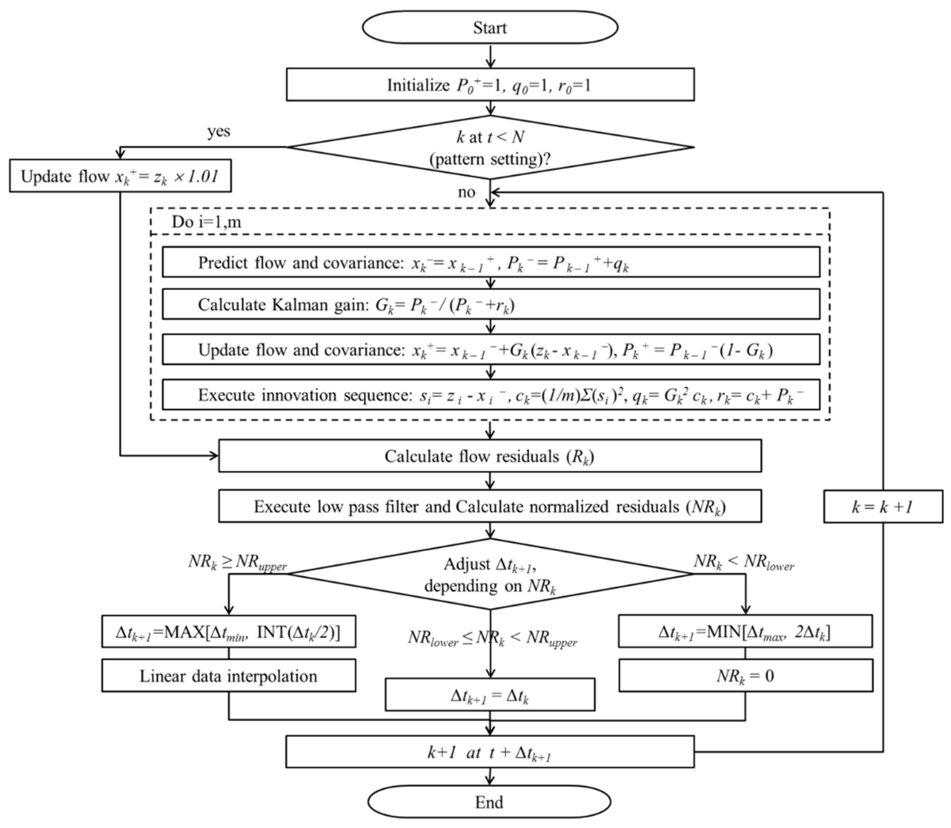
2.1. Kalman Filtering

The Kalman filter is a linear algorithm that estimates the internal state of a system. It operates recursively on streams of noisy input data to produce an optimal estimate of the underlying system state [15]. It has found wide application in tasks such as process control, sensor fusion, motion tracking, and neural information processing. The Kalman filter is essentially a set of mathematical equations that implement a predictor-corrector type of estimator that is optimal in the sense that it minimizes the estimated error covariance when the condition of a linear Gaussian system is met.

In the application to burst detection in a WDS, it is assumed that the state variable of the flow, $x$, is a constant in that the current value at time step $k$ is set equal to the previous value at time step $k-1$ as follows:

$$x_k=x_{k-1}+w_k , w_k~N\left(0,q_k\right)$$

(1)

where $w$ denotes the process noise, which has a zero-mean normal distribution with covariance $q$. The measurement of the flow, $z$, can be made as follows:

$$z_k=x_k+v_k , v_k~N\left(0,r_k\right)$$

(2)

where $v$ is the measurement noise, which is zero-mean Gaussian white noise with covariance $r$.

The Kalman filter consists of three major steps as shown in Figure 1. In the prediction step, the filter estimates the internal state at the next time step, along with its uncertainties, as follows:

$$x_k^{-}=x_{k-1}^{+} , P_k^{-}=P_{k-1}^{+}+q_k$$

(3)

where $P$ is the estimated covariance, and superscripts $-$ and $+$ represent the predictor (predicted variable) and the corrector (updated variable), respectively. Then, the Kalman gain $G$ is calculated with the following equation:

$$G_k=P_k^{-}/\left(P_k^{-}+r_k\right)$$

(4)

In the final update step, the estimate and covariance are updated by minimizing the error covariance under the influence of external observations as follows:

$$x_k^{+}=x_k^{-}+G_k\left(z_k-x_k^{-}\right) , P_k^{+}=P_k^{-}\left(1-G_k\right)$$

(5)

2.2. Adaptive Method with Adjustable Sampling Interval

In applications of the Kalman filter, the inaccurate information of noise can decrease the quality of estimation, thus the covariances of noise, $q$ and $r$, should be repeatedly updated. In this paper, the so-called innovation sequence [13,16] is adopted to yield an unbiased estimate through its automatic tuning process. As shown in Figure 1, the innovation covariance, $c$, is calculated as:

$$c_k=\left({\displaystyle \sum }_{i=k-m+1}^k{s}_i^2\right)/m$$

(6)

where $s_i=z_i-x_i^{-}$ and $m$ denotes the number of iterations (which is set to five in this study). The $c$ obtained is utilized to calculate the iteratively updated covariances of noise as follows:

$$q_k=G_k^2{c}_k , r_k=c_k+P_k^{-}$$

(7)

The water flow in a DMA is inherently unsteady due to continuously varying demand. The temporal variations in water usage for municipal water systems follow a 24-h cycle called a diurnal demand pattern. However, the system flow experiences changes not only on a daily basis but also weekly and annually. The seasonal pattern has been related to climatic variables and the habits of customers. However, its modeling requires not only an inference engine but also many associated data, such as those on DMA flow, temperature, and precipitation. Therefore, seasonal variation is not considered in this study. Instead, daily and weekly usage patterns are incorporated by assuming that the current flow is similar to that of the previous week at the corresponding time. In other words, if the number of flow data collected in a week is $N$ (also called the number of pattern setting data), then $x_{k-N}^{+}$ and $P_{k-N}^{+}$ replace $x_{k-1}^{+}$ and $P_{k-1}^{+}$ as the previous values of the estimate and covariance that are employed in Equation (3) to predict the current values.

While applying the Kalman filter, a burst can be detected by calculating a flow residual as follows:

$$R_k=z_k-x_k^{+}$$

(8)

However, the calculated residual can hinder detecting a burst when a high magnitude of noise between the Kalman predicted flow and the measured value, comparable to a burst event, is recorded. In this study, therefore, the following low-pass filter is utilized to obtain smoother normalized forms of residual curves:

$$N{R}_k=\left(LPF{z}_k-LPF{x}_k^{+}\right)/LPF{z}_k$$

(9)

where LPF denotes the low-pass filtering by a moving average, and has a 1-week window size drawn from the assumption that the current value of week $k$ is closely related to the previous value of week $k-1$. Once a normalized residual is obtained from Equation (9), an adjustable sampling interval, $\Delta t$, is tuned in accordance with the magnitude of the residual as follows:

$$\Delta t_{k+1}=\{\begin{array}{c} MAX\left[\Delta t_{min} , INT\left(\Delta t_k/2\right) \right] if N{R}_k\ge N{R}_{upper} \\ \Delta t_k if N{R}_{lower}\le N{R}_k<N{R}_{upper}\\ MIN\left[\Delta t_{max} ,2\Delta t_k\right] if N{R}_k<N{R}_{lower} \end{array}$$

(10)

where MAX and MIN denote the maximum and minimum value inside the bracket, respectively, INT is an integer operator that rounds off to the nearest value, and $\Delta t_{min}$ and $\Delta t_{max}$ denote the minimum and maximum sampling intervals, respectively, defined by the user, while also considering practical application. Note that $N{R}_{lower}$ and $N{R}_{upper}$ denote lower and upper thresholds that are empirical constants depending on the characteristics of the flow data. In this study, 0.01 and 0.015 are employed as the lower and upper values by using iterative simulations while the sensitivity of the $\Delta t_{k+1}$ changes are being monitored. Moreover, a residual less than $N{R}_{lower}$ is set to zero, because a negative residual indicates that the real water demand is greater than the estimated flow and because an extremely small residual is negligible in practice. In applications of the proposed method, missing values of the measurement and estimate are encountered if the sampling interval decreases, because the filter needs information on the same time in the previous week to estimate the current flow. Therefore, four values that are adjacent in time are utilized to produce an interpolated value using Lagrange’s polynomial at the corresponding time.

3. Results and Discussion

In this section, the effect of sampling interval is first investigated in terms of estimation accuracy for burst detection with the adaptive Kalman filter. For this purpose, the filter is applied to virtual sinusoidal flow data with sampling intervals ranging from 1 to 60 min, and the residuals are compared. Then, the same flow data are utilized to investigate the effect of an adjustable sampling interval. Finally, the in situ flow data measured in two DMAs of JE (a city in South Korea) are used to test the suitability of the method for real applications. In practice, the data obtained from SCADA systems can contain errors caused by system failures of power and communication, or by scheduled downtime in the system. Therefore, it is inferred that a short sampling interval (e.g., 1 min) is more likely to feature outliers or missing data than a long one (e.g., 60 min). As for the outliers, statistical tests can be applied to detect them according to sample size, assumption of normal distribution, and detection of multiple outliers [17,18]. The detected outliers and missing values can be further handled with imputation, partial imputation, partial deletion, full analysis and interpolation. The 1-min results are potentially the best indicator of bursts and so here are used as reference data. However, the 1-min results could be overly sensitive and so include many false positives.

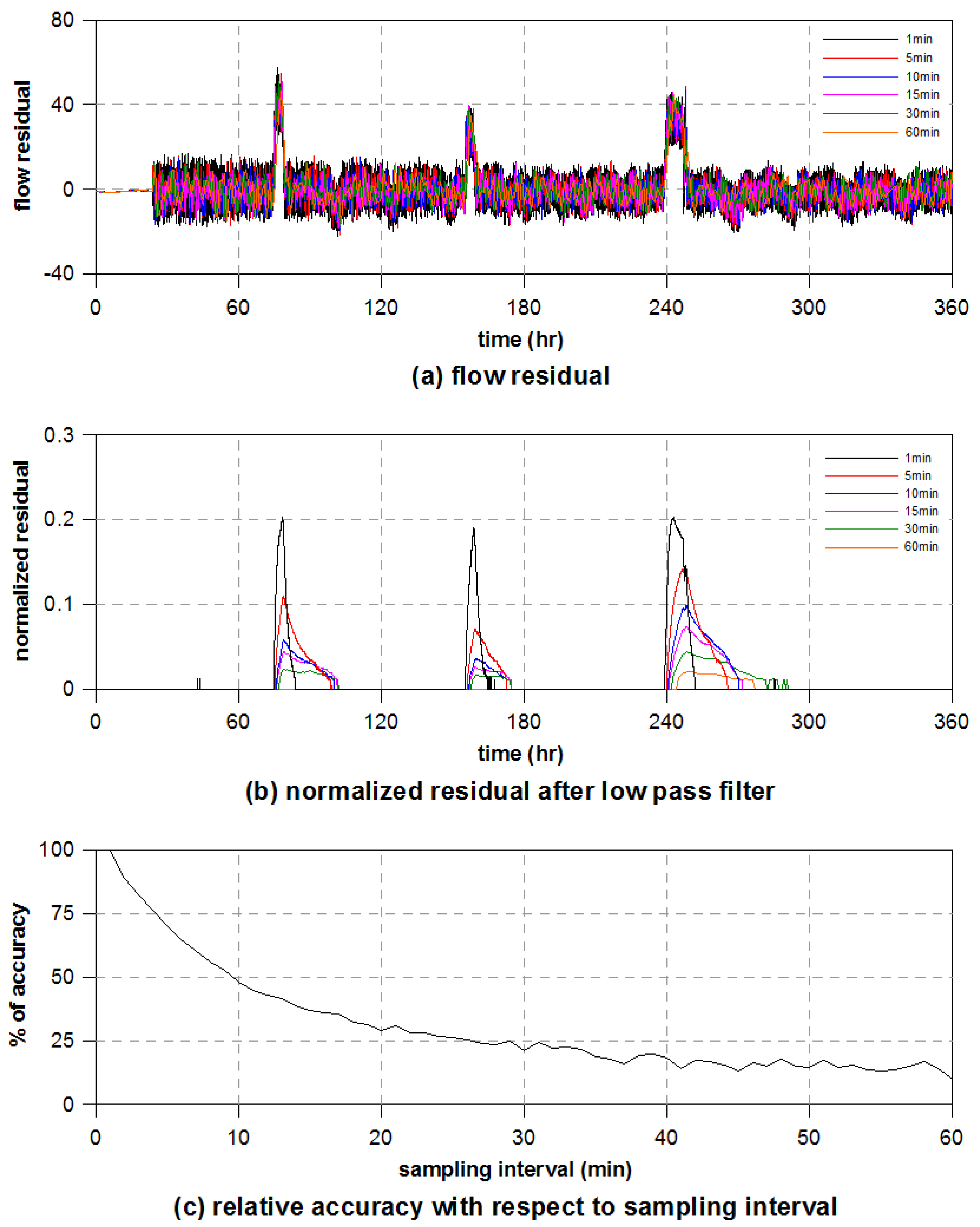
3.1. Effect of Sampling Interval

For convenience of verification, flow data are generated by analytical and numerical methods, as shown in Figure 2. The composite sinusoidal flow in Figure 2d has three components: a sine curve, three trapezoidal bursts, and random noise. The sine curve is first defined as

$$Flo{w}_t=40\sin \left(2\pi t/24\right)+100$$

(11)

where $t$ denotes time. The above flow curve has an average of 100 and amplitude of 40 (Figure 2a). In general, a burst causes a gradual increase in DMA flow during the onset before full development and a gradual decrease during the repair period. Therefore, a trapezoidal shape is chosen for burst curves. The trapezoidal bursts have peak flows of 50 for 74 h ≤ t ≤ 79 h, 30 for 155 h ≤ t ≤ 159 h, and 40 for 238 h ≤ t ≤ 247 h (Figure 2b). A random noise equal in amplitude to 5% of the average flow is added with a random number generator (Figure 2c). To investigate the effect of sampling interval on burst detection, a series of flow data is generated for time intervals from 1 to 60 min.

The flow residuals calculated with the adaptive Kalman filtering are shown in Figure 3a according to the sampling intervals of the datasets. At the beginning of the simulation, the flow residual is almost zero, because in the first cycle the estimate is set to $1.01\times z_k$, which is known as the number of pattern setting data. In addition, the residuals calculated from Equation (8) contain negative values due to the low-amplitude noise. Figure 3a shows that the three burst events can be clearly distinguished from the noise, but the results are vulnerable to false alarms because of the random noise. In contrast, Figure 3b shows that the normalized flow residuals calculated from Equation (9) are devoid of the random noise. Although the normalized residuals after the process of low-pass filtering have smaller values, the bursts can be detected more clearly without any random noise. It is also found that a larger sampling interval provides bursts of longer duration and peaks of smaller magnitude. In field applications, the flow data include several types of noise, leaks, and bursts, so the smooth residual curves at larger sampling intervals cannot be effective in detecting bursts. Figure 3c shows the relative accuracy, which is the percentage ratio of the given residual to the 1-min residual with respect to the magnitude of the peak. It is found that the accuracy decreases exponentially as the sampling interval increases.

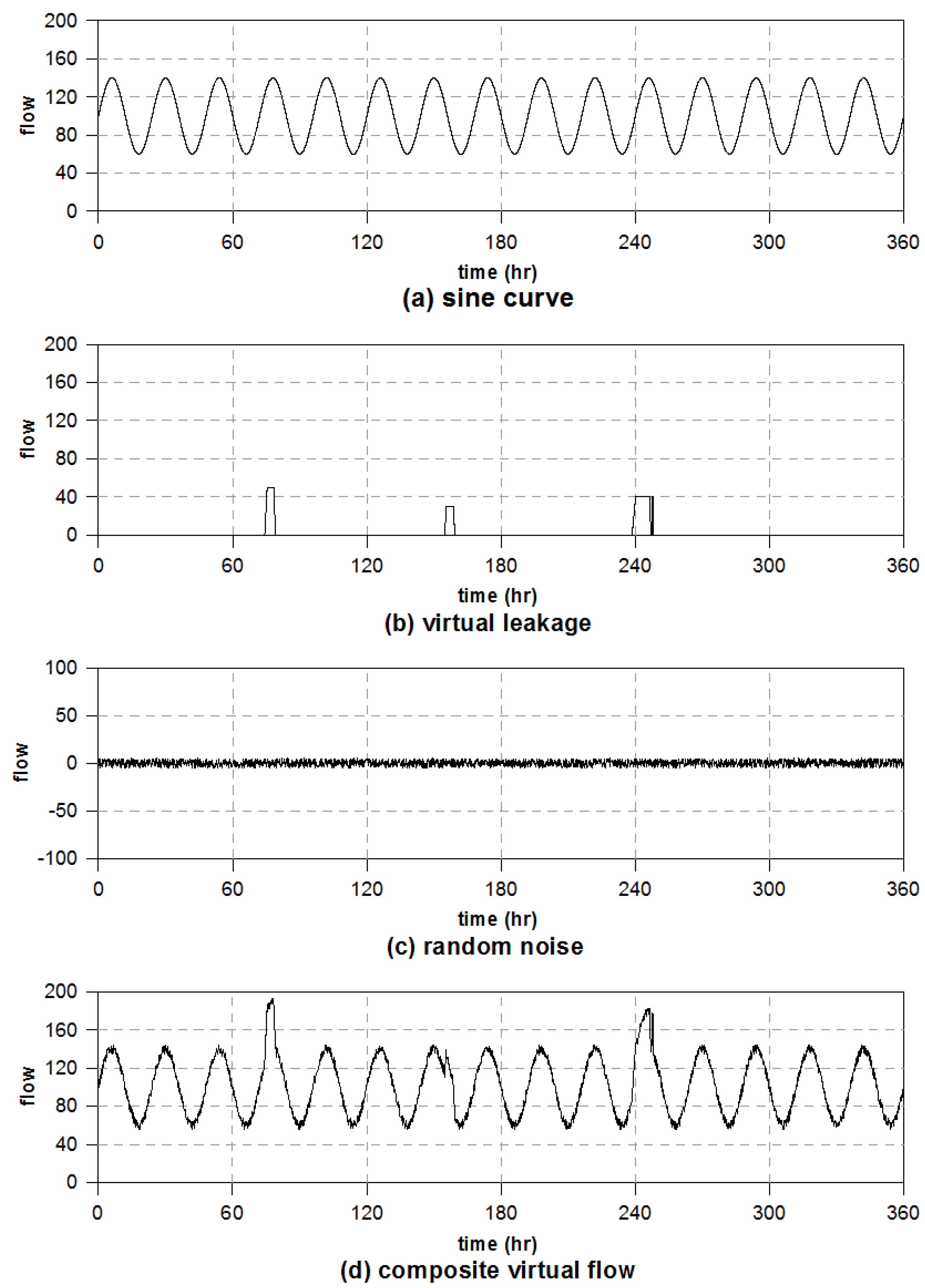
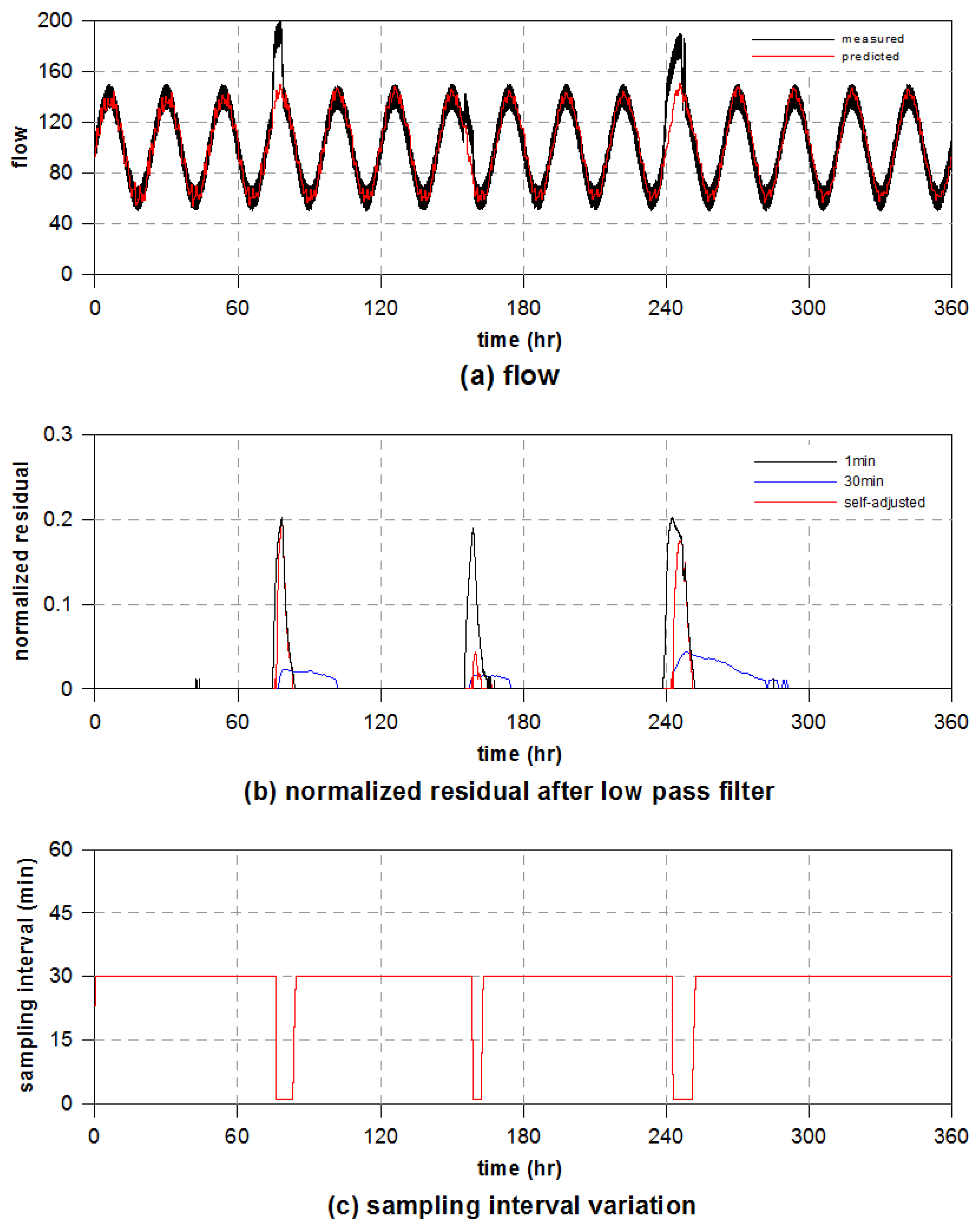
3.2. Application of Self-Adjusting Method to Virtual Flow Data

In order to validate the proposed self-adjusting method for the sampling interval, the same flow curve was employed. In order to implement the proposed method, two sets of criteria should be specified; i.e., one for the sampling interval and one for the normalized residuals. In this study, minimum and maximum sampling intervals of 1 and 30 min were specified, respectively. As stated above, the lower and upper thresholds of the normalized residual were set to 0.01 and 0.015, respectively. At the beginning of the filtering process, the sampling interval is set to 30 min, as that is the maximum sampling interval. Figure 4a shows the results predicted with the self-adjusting algorithm and the virtual data. In addition, Figure 4b shows the normalized residuals after low-pass filtering together with those for constant sampling intervals of 1 and 30 min. The proposed method exhibits its capability to clearly detect two burst events with normalized residuals of high magnitude, which are much more comparable to the 1-min results than the 30-min results. Although the peak of the second burst event is subdued, the result shows the advantage of the model for burst detection by resolving the short duration of the burst. Figure 4c shows the variation in the sampling interval with the simulation time under the conditions of Equation (10). As seen in the figure, the proposed method utilizes high-frequency data only when burst events are detected. By doing so, the self-adjusting approach limits its total number of data to 1806, which is a remarkably small number compared to the 21,601 samples used at 1-min intervals and is only 2.5 times the 721 samples used at 30-min intervals. Overall, the simulation results prove that the self-adjusting method for the sampling interval can be applicable in detecting burst events efficiently without significant losses of accuracy.

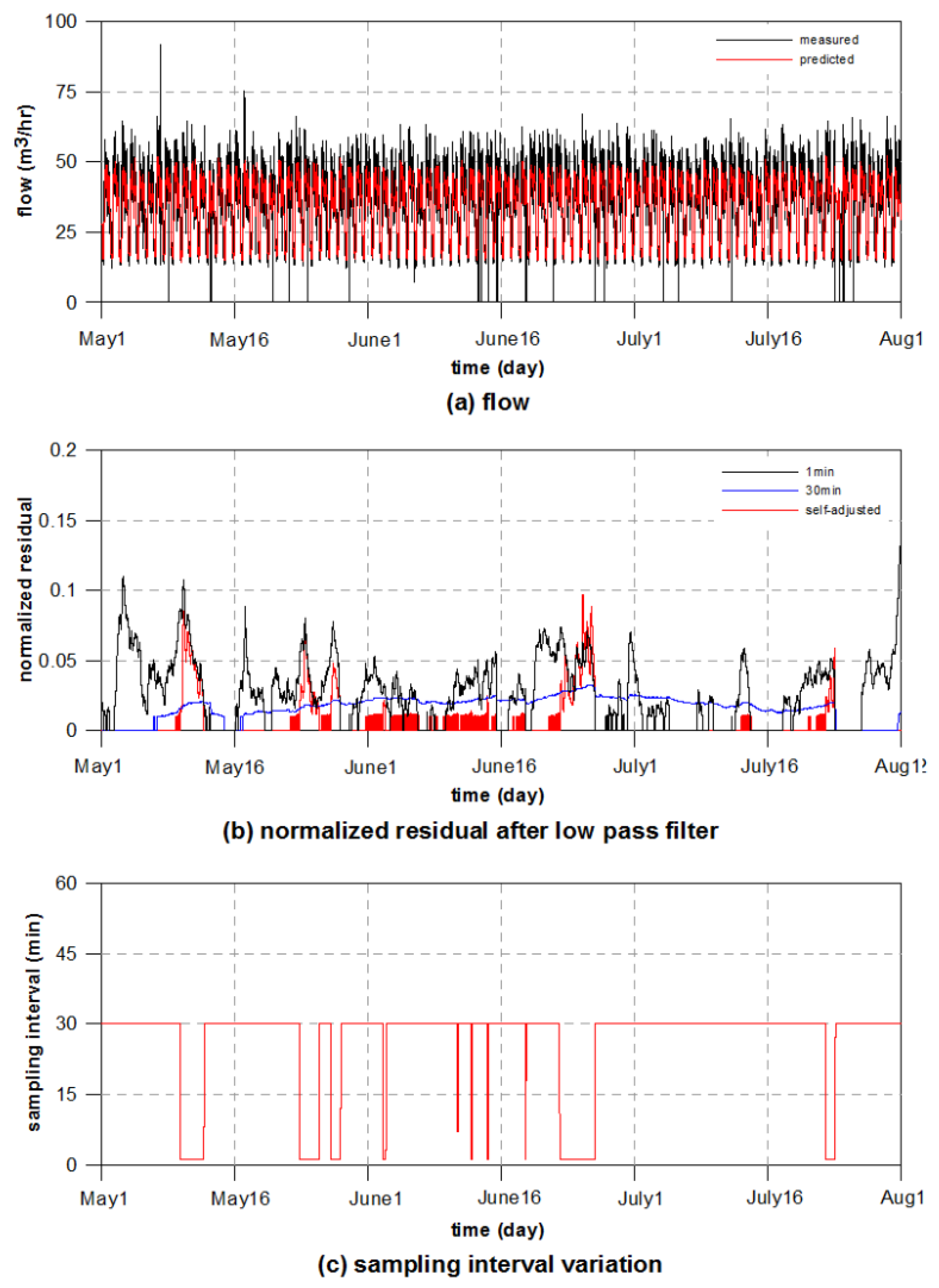
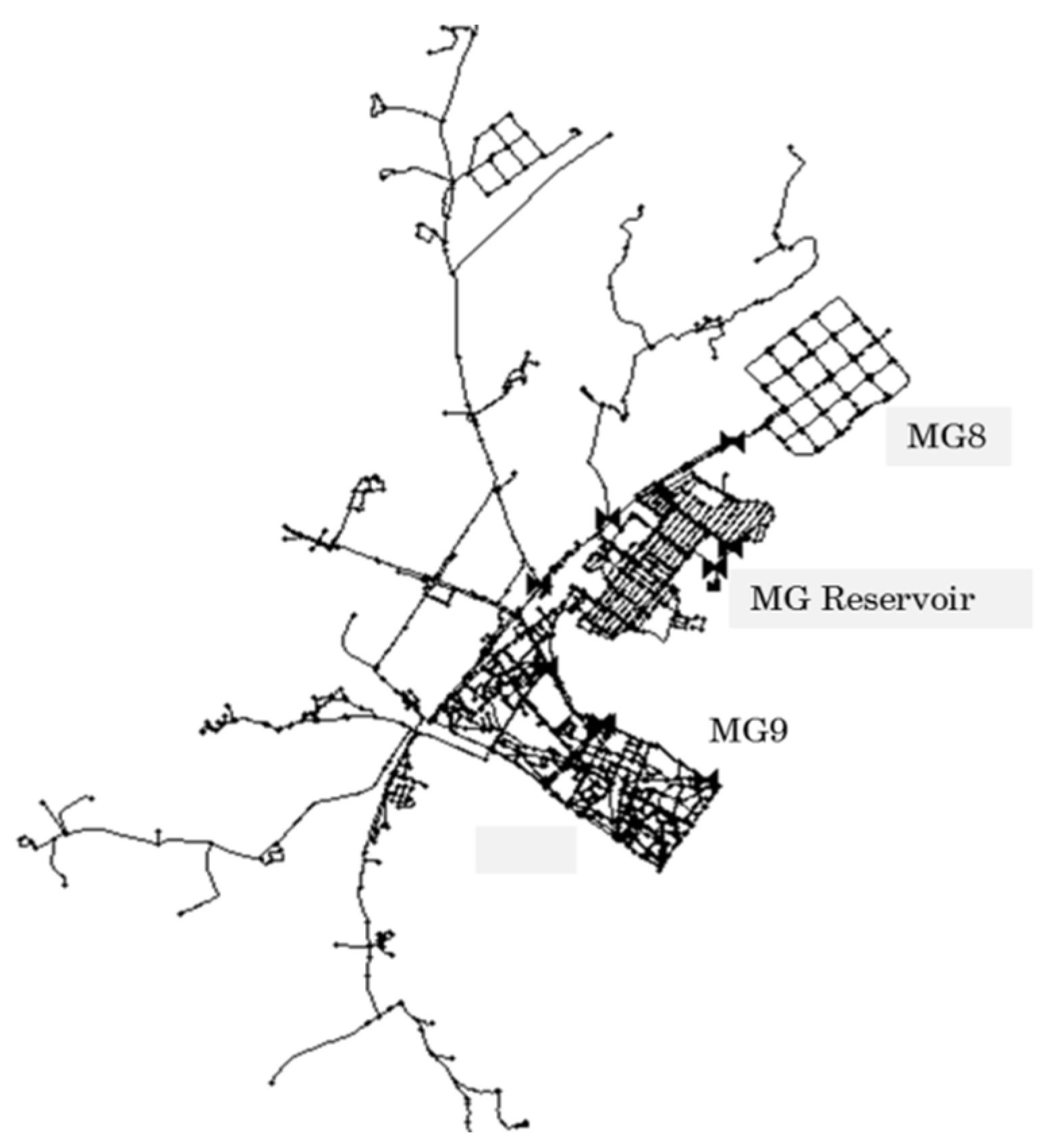
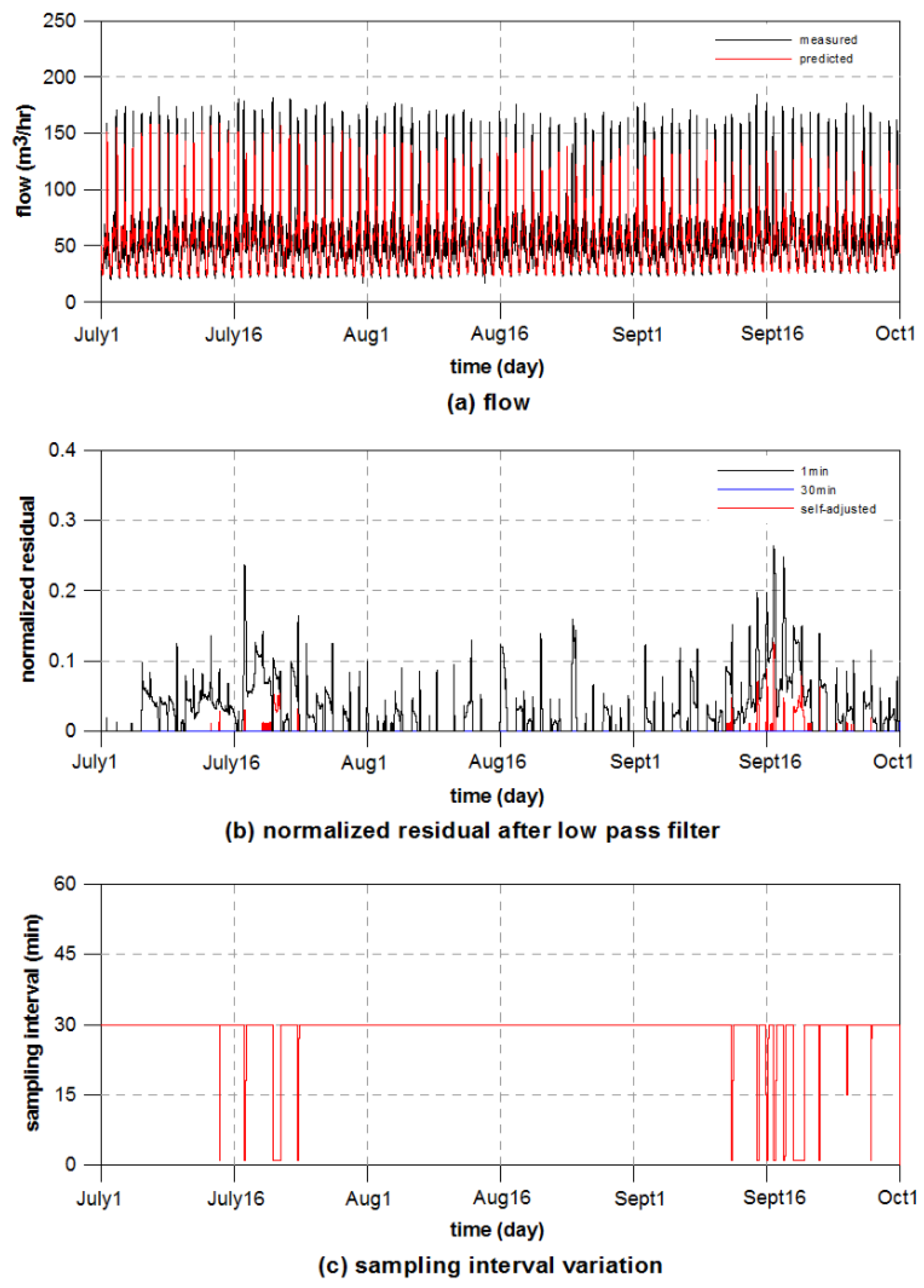
3.3. Application of Self-Adjusting Method to Real DMA Flow Data

The developed algorithm was applied to real flow data on two DMAs selected from JE, a city in South Korea. The water in the DMAs is distributed from the Magok (MG) reservoir, which is one of the reservoirs supplied from the JE water treatment plant, as shown in Figure 5. Two 3-month periods were considered in this study: from 1 May to 31 July for MG8, and from 1 July to 30 September for MG9. The flow data were actually measured with a sampling interval of 1 min, but only those data required by the adjustable sampling interval were utilized in the simulation. For simulations with real DMA data, minimum and maximum sampling intervals of 1 and 30 min were specified, respectively. Figure 6a and Figure 7a show the flow measurement time series and the flow results predicted with the self-adjusting algorithm. Figure 6b and Figure 7b show the potential burst detection results expressed as normalized residuals for 1-min, 30-min, and adjustable time intervals. Figure 6c and Figure 7c show the variation in the sampling interval over time when the self-adjusting algorithm was implemented.

In DMA MG8, the flow ranges from 15 to 60 m³/h with a small deviation from the average of 35.3 m³/h, as shown in Figure 6a. In the measured data, abnormally large flow rates of 92 and 75 m³/h are observed in May, and many zero values are found over the measurement period. This dataset cannot be regarded as one qualified for detecting bursts with a reasonable accuracy. However, the simulation results can be useful, because the main purpose is to compare the sensitivity and efficiency of sampling intervals. The normalized residuals after low-pass filtering, which are calculated from Equation (9), are plotted in Figure 6b for three types of sampling intervals. As predicted from the many zero flow rates, many bursts are detected over the simulation period. According to the results for a constant 30-min sampling interval, the burst alarm should be provided over almost the whole sampling period. In contrast, the self-adjusting algorithm provides intermittent burst alarms with the distinct magnitude peaks of the normalized residuals. As shown in Figure 6c, the sampling interval remains at 30 min (i.e., the maximum sampling interval) in most of the simulation, but more frequent sampling is requested when detecting bursts.

In DMA MG9, the flow ranges from 25 to 160 m³/h with a large deviation from the average of 58.1 m³/h, as shown in Figure 7a. Unlike the flow data observed in DMA MG8, those observed in DMA MG9 are consistent over the sampling period, without missing or abnormal values. In the measured data, a high flow rate in excess of 150 m³/h is reached, which is a relatively large amount compared with the average flow rate of 58.1 m³/h. This can be explained by a large amount of commercial water use in the daytime. The potential bursts were clearly detected with normalized residuals at 1-min and adjustable sampling intervals. However, no bursts were detected with a constant 30-min sampling interval, because this is too rough to carry noise information. Although the self-adjusting algorithm overlooked the bursts detected in the 1-min prediction from July to September, its superiority over the 30-min sampling interval can be demonstrated. Moreover, only 9486 samples were utilized for burst prediction, which is only twice as many samples as with 30-min interval (

Table 1. Summary of simulation results for actual DMA data.

DMA	Alarms			Samples
	1 min	30 min	Self-Adjusted	1 min	30 min	Self-Adjusted
MG8	38	5	19	132,481	4416	21,003
MG9	73	0	20	132,481	4416	9486

). As shown in Table 1, the overall results of detecting bursts with the self-adjusting algorithm proved the application successful with respect to accuracy and efficiency that are expressed as numbers of alarms and samples, respectively. The number of alarms was counted by setting the alarm threshold to be 0.01 of the threshold value of $N{R}_k$.

4. Conclusions

In this study, the sampling interval of a flow meter installed in the inlet of a DMA for detecting pipeline bursts was addressed. An adaptive Kalman filter algorithm that incorporates an adjustable sampling interval was presented by introducing maximum and minimum sampling intervals and upper and lower thresholds for normalized residuals. To stress the effect of the sampling interval, a computational experiment was performed for virtual flow data composed of a sine curve, trapezoidal bursts, and random noise. The results showed that a larger sampling interval generates bursts of longer duration and peaks of smaller magnitude. The proposed sampling algorithm was then tested with two applications: a virtual sinusoidal flow curve and real DMA flow curves obtained from JE (a city in South Korea). For the virtual flow data, the suggested method showed its efficiency by resolving short duration bursts, which was close to a simulation with a 1-min sampling interval, although the peak of the second burst event was subdued. In the application to two real DMAs (MG8 and MG9), the self-adjusting algorithm called 19 and 20 alarms for MG8 and MG9, respectively. These numbers of alarms, which indirectly relate to accuracy, are equivalent to 27%–50% of the alarms in a simulation with a 1-min sampling interval. Regarding the sampling efficiency, which is expressed as the number of samples, the proposed model required 21,003 and 9486 samples for MG8 and MG9, respectively. These sample numbers are equivalent to 7%–16% of the alarms in a simulation with a 1- min sampling interval.

Note that the proposed algorithm has an innate limitation in that it cannot discern between abnormal water demands and breaks or leaks in pipes because it uses an adaptive Kalman filter as a burst estimator. However, the self-adjusting algorithm for the sampling interval can be combined with other models, such as an artificial neural network, for predicting only pipe bursts. It is also concluded that the proposed algorithm has a significant potential for water utilities to build and operate real-time DMA monitoring systems and SCADA systems in an efficient way. Moreover, the suggested algorithm will be more effective when the real-time DMA flow is considered for managing nonrevenue water with a smart customer metering system.

References

1. Farley, B.; Mounce, S.R.; Boxall, J.B. Field testing of an optimal sensor placement methodology for event detection in an urban water distribution network. Urban Water J. 2010, 7, 345–356. [Google Scholar] [CrossRef]
2. Lambert, A. Accounting for losses: the bursts and background concept. Water Environ. J. 1994, 8, 205–214. [Google Scholar] [CrossRef]
3. Giurco, D.P.; White, S.B.; Stewart, R.A. Smart metering and water end-use data: Conservation benefits and privacy risks. Water 2010, 2, 461–467. [Google Scholar] [CrossRef]
4. Liggett, J.A.; Chen, L.C. Inverse transient analysis in pipe networks. J. Hydraul. Eng. 1994, 120, 934–955. [Google Scholar] [CrossRef]
5. Covas, D.; Ramos, H.; de Almeida, A.B. Standing wave difference method for leak detection in pipeline systems. J. Hydraulic Eng. 2005, 131, 1106–1116. [Google Scholar] [CrossRef]
6. Anderson, J.H.; Powell, R.S. Implicit state-estimation technique for water network monitoring. Urban Water 2000, 2, 123–130. [Google Scholar] [CrossRef]
7. Poulakis, Z.; Valougeorgis, D.; Papadimitriou, C. Leakage detection in water pipe networks using a Bayesian probabilistic framework. Probabilistic Eng. Manag. 2003, 18, 315–327. [Google Scholar] [CrossRef]
8. Puust, R.; Kapelan, Z.; Savic, D.A.; Koppel, T. Probabilistic leak detection in pipe networks using the SCEM-UA algorithm. In Proceedings of the 8th Annual Water Distribution Systems Analysis Symposium, Cincinnati, OH, USA, 27–30 August 2006.
9. Palau, C.V.; Arregui, F.J.; Carlos, M. Burst detection in water networks using principal component analysis. J. Water Resour. Plan. Manag. 2012, 138, 47–54. [Google Scholar] [CrossRef]
10. Mounce, S.R.; Machell, J. Burst detection using hydraulic data from water distribution systems with artificial neural networks. Urban Water J. 2006, 3, 21–31. [Google Scholar] [CrossRef]
11. Aksela, K.; Aksela, M.; Vahala, R. Leakage detection in a real distribution network using a SOM. Urban Water J. 2009, 6, 279–289. [Google Scholar] [CrossRef]
12. Mounce, S.R.; Boxall, J.B.; Machell, J. Development and verification of an online artificial intelligence system for detection of bursts and other abnormal flows. J. Water Resour. Plan. Manag. 2012, 136, 309–318. [Google Scholar] [CrossRef]
13. Ye, G.; Fenner, R.A. Kalman filtering of hydraulic measurements for burst detection in water distribution systems. J. Pipeline Syst. Eng. Pract. 2011, 2, 14–22. [Google Scholar] [CrossRef]
14. Ye, G.; Fenner, R.A. Study of burst alarming and sampling frequency in water distribution networks. J. Water Resour. Plan. Manag. 2014, 140, 06014001. [Google Scholar] [CrossRef]
15. Kalman, R.E. A new approach to linear filtering and prediction problems. J. Basic Eng. 1960, 82, 35–45. [Google Scholar] [CrossRef]
16. Mehra, R.K. On the identification of variances and adaptive Kalman filtering. Automatic Control 1970, 15, 175–184. [Google Scholar] [CrossRef]
17. Berthouex, P.M.; Brown, L.C. Statistics for Environmental Engineers, 2nd ed.; Lewis Publishers: Boca Raton, FL, USA, 2002. [Google Scholar]
18. US Environmental Protection Agency (US EPA). Data Quality Assessment: Statistical Methods for Practitioners; Report No. EPA QA/G-9S; US EPA: Washington, DC, USA, 2006.
Figure 1. Procedure for detecting bursts with adaptive Kalman filter incorporating adjustable sampling interval.
Water 08 00142 g001
Figure 2. Virtual flow data: (a) sine curve; (b) virtual leakage; (c) random noise; and (d) composite virtual flow.
Water 08 00142 g002
Figure 3. Burst detection results with respect to sampling interval for virtual flow data: (a) flow residual; (b) normalized residual after low-pass filtering; and (c) relative accuracy versus sampling interval.
Water 08 00142 g003
Figure 4. Burst detection results with adjustable sampling interval for virtual flow data: (a) flow; (b) normalized residual after low-pass filtering; and (c) sampling interval variation.
Water 08 00142 g004
Figure 5. Schematic layout of MG DMAs in JE.
Water 08 00142 g005
Figure 6. Burst detection results with adjustable sampling interval for DMA MG8: (a) flow; (b) normalized residual after low-pass filtering; and (c) sampling interval variation.
Water 08 00142 g006
Figure 7. Burst detection results with adjustable sampling interval for DMA MG9: (a) flow; (b) normalized residual after low-pass filtering; and (c) sampling interval variation.
Water 08 00142 g007