
Spatial and Temporal Correlates of Greenhouse Gas Diffusion from a Hydropower Reservoir in the Southern United States

Abstract
:1. Introduction
2. Materials and Methods
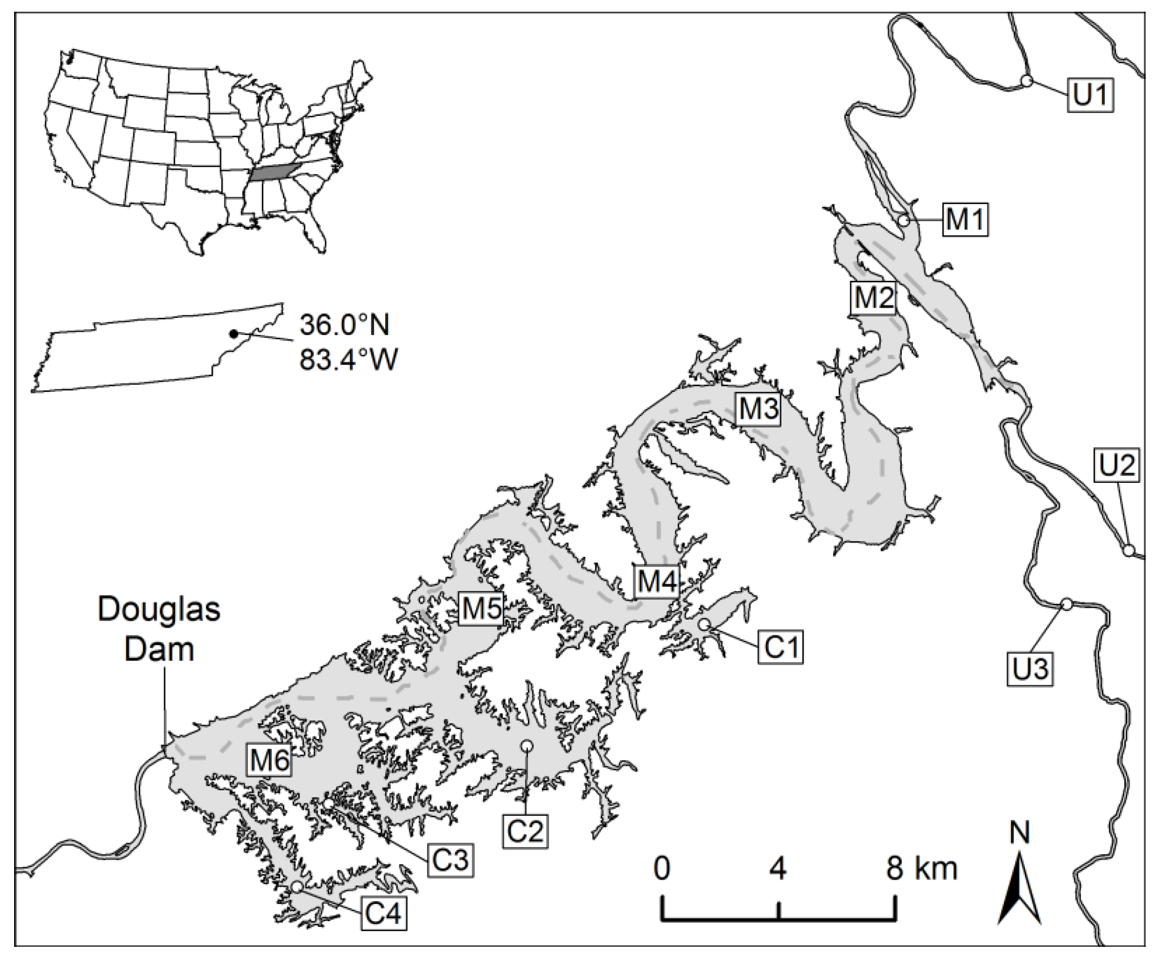
2.1. Study Site and Field Sampling
2.2. CO2 and CH4 Emissions and Physicochemical Variables
2.3. Data Analysis

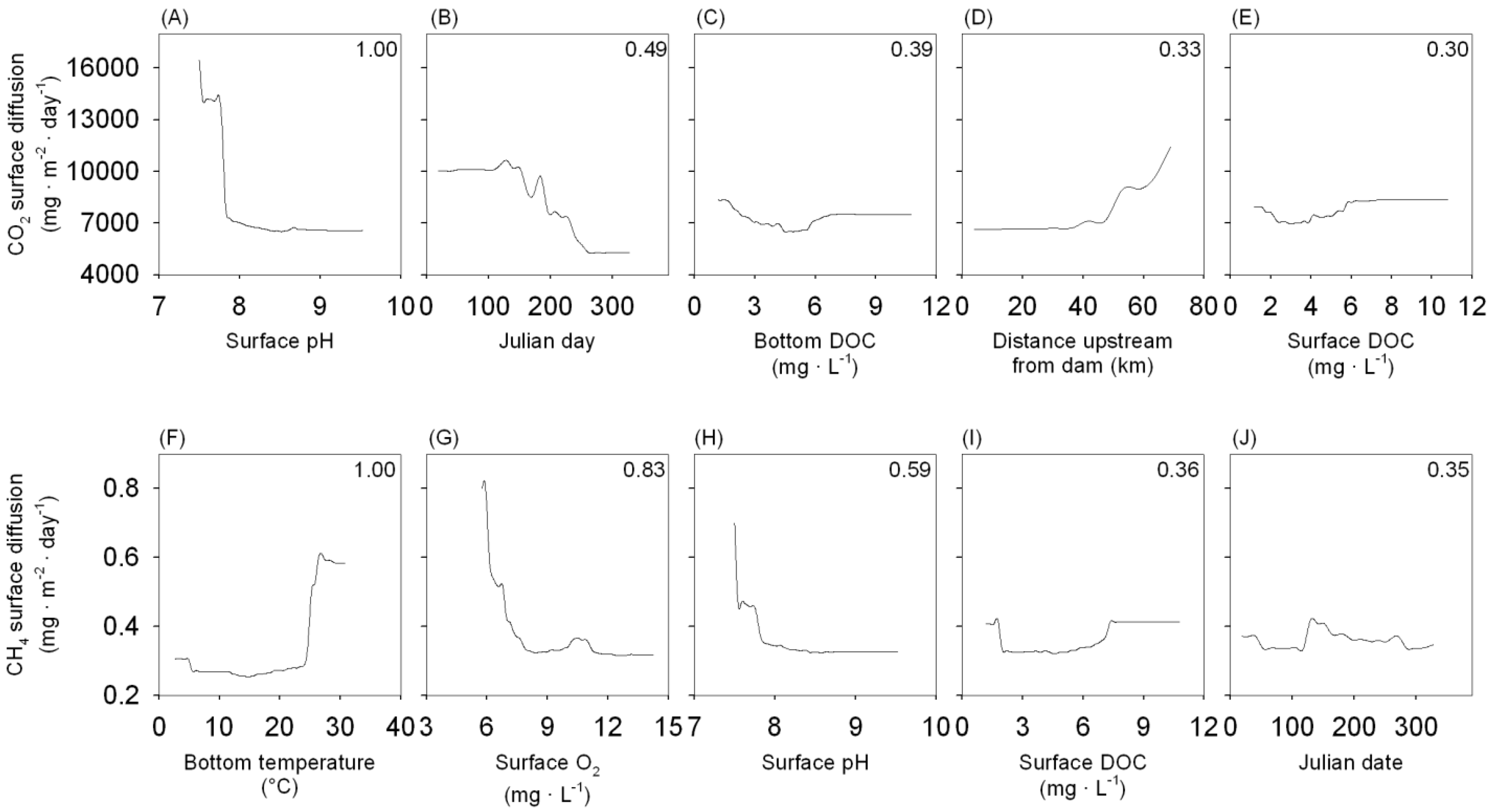
| Predictor | CO2 | CH4 |
|---|---|---|
| Julian day | 0.49 | 0.35 |
| Longitudinal position | 0.33 | 0.01 |
| Depth | 0.06 | 0 |
| O2 bottom concentration | 0 | 0.12 |
| DOC bottom concentration | 0.39 | 0.17 |
| NH4+ bottom concentration | 0.29 | 0.11 |
| NO3– bottom concentration | 0.11 | 0.07 |
| pH bottom | 0.2 | 0.05 |
| SRP bottom | 0.03 | 0.16 |
| Temperature bottom | 0.08 | 1 |
| O2 surface concentration | 0.28 | 0.83 |
| DOC surface concentration | 0.3 | 0.36 |
| NH4+ surface concentration | 0.01 | 0.03 |
| NO3– surface concentration | 0.27 | 0.11 |
| pH surface | 1 | 0.59 |
| SRP surface | 0.13 | 0.17 |
3. Results and Discussion
3.1. Physicochemical Conditions of Douglas Lake
| Variable | M1 | M2 | M3 | M4 | M5 | M6 | C1 | C2 | C3 | C4 | U1 | U2 | U3 |
|---|---|---|---|---|---|---|---|---|---|---|---|---|---|
| Depth (m) | 2.5 | 7.9 | 9.5 | 11.8 | 20.0 | 25.2 | 10.1 | 15.7 | 4.8 | 11.8 | 1.5 | 1.5 | 1.5 |
| (0.3) | (1.5) | (2.3) | (2.3) | (3.3) | (2.5) | (2.4) | (1.6) | (1.9) | (2.7) | (NA) | (NA) | (NA) | |
| Surface temperature (°C) | 27.6 | 27.6 | 23.6 | 23.2 | 23.1 | 20.7 | 23.0 | 23.0 | 20.8 | 22.0 | 23.7 | 20.9 | 20.3 |
| (2.3) | (1.9) | (4.9) | (5.0) | (4.7) | (5.9) | (5.1) | (4.8) | (5.6) | (6.4) | (4.4) | (4.6) | (3.8) | |
| Bottom temperature (°C) | 26.7 | 24.8 | 20.3 | 19.8 | 16.7 | 14.5 | 19.0 | 18.9 | 20.1 | 17.9 | 23.7 | 20.9 | 20.3 |
| (2.8) | (1.4) | (4.3) | (3.6) | (4.1) | (4.2) | (4.5) | (4.7) | (5.4) | (5.0) | (4.4) | (4.6) | (3.8) | |
| Surface O2 (mg·L−1) | 7.4 | 7.9 | 10.0 | 9.6 | 9.5 | 9.5 | 9.6 | 9.5 | 9.7 | 10.0 | 8.9 | 8.6 | 8.8 |
| (1.4) | (1.0) | (1.5) | (1.0) | (1.3) | (1.4) | (1.5) | (1.5) | (1.5) | (1.9) | (1.5) | (0.9) | (0.9) | |
| Bottom O2 (mg·L−1) | 6.8 | 5.0 | 4.0 | 3.1 | 4.8 | 4.1 | 4.6 | 5.6 | 8.8 | 5.9 | 8.9 | 8.6 | 8.8 |
| (0.6) | (2.4) | (2.8) | (2.2) | (2.7) | (2.5) | (3.1) | (2.5) | (2.1) | (3.4) | (1.5) | (0.9) | (0.9) | |
| Surface pH | 8.16 | 8.06 | 8.55 | 8.47 | 8.46 | 8.00 | 8.63 | 8.37 | 7.96 | 8.33 | 8.27 | 7.96 | 8.2 |
| (NA) | (0.44) | (0.42) | (0.45) | (0.48) | (0.31) | (0.22) | (0.54) | (0.29) | (0.36) | (0.43) | (0.43) | (0.35) | |
| Bottom pH | 8.13 | 7.61 | 7.63 | 7.33 | 7.44 | 7.28 | 7.81 | 8.07 | 7.88 | 7.81 | 8.27 | 7.96 | 8.20 |
| (NA) | (0.31) | (0.25) | (0.42) | (0.28) | (0.20) | (0.36) | (0.26) | (0.17) | (0.37) | (0.43) | (0.43) | (0.35) | |
| Surface DOC (mg·L−1) | 2.1 | 2.6 | 2.8 | 3.3 | 3.0 | 2.8 | 3.4 | 3.1 | 2.9 | 2.7 | 4.6 | 3.4 | 4.9 |
| (0.5) | (0.4) | (1.1) | (1.1) | (1.3) | (1.2) | (1.4) | (1.3) | (1.2) | (0.9) | (3.0) | (1.4) | (1.7) | |
| Bottom DOC (mg·L−1) | 2.3 | 2.5 | 4.3 | 4.0 | 6.7 | 1.7 | 6.9 | 5.0 | 1.8 | 5.8 | 4.6 | 3.4 | 4.9 |
| (0.4) | (0.9) | (4.7) | (2.8) | (1.6) | (NA) | (NA) | (3.6) | (0.4) | (NA) | (3.0) | (1.4) | (1.7) | |
| Surface NH4+ (μg N·L−1) | 43.3 | 78.3 | 29 | 22.2 | 11.7 | 17.5 | 27.2 | 14.1 | 24.9 | 18.8 | 21.7 | 20.5 | 15.7 |
| (20.5) | (64.9) | (18.3) | (12.0) | (8.5) | (10.1) | (13.5) | (7.7) | (14.4) | (12.1) | (12.8) | (20.9) | (7.4) | |
| Bottom NH4+ (μg N·L−1) | 46.3 | 327.0 | 447.7 | 406.0 | 338.3 | 57.6 | 81.5 | 26.7 | 23.3 | 12.0 | 21.7 | 20.5 | 15.7 |
| (19.5) | (348.2) | (352.1) | (331.7) | (603.5) | (NA) | (NA) | (22.7) | (14.6) | (NA) | (12.8) | (20.9) | (7.4) | |
| Surface NO3− (μg N·L−1) | 241.4 | 356.8 | 110.7 | 108.3 | 111.7 | 169.6 | 77.7 | 176.1 | 174.6 | 176.1 | 357.3 | 536.2 | 356.4 |
| (112.4) | (236.9) | (100.2) | (81.7) | (90.2) | (119.3) | (65.4) | (118.3) | (119.1) | (126.9) | (126.5) | (122.0) | (78.6) | |
| Bottom NO3− (μg N·L−1) | 251.9 | 485.9 | 222.0 | 261.4 | 138.4 | 47.8 | 70.1 | 220.5 | 112.1 | 62.0 | 357.3 | 536.2 | 356.4 |
| (138.4) | (137.1) | (370.5) | (197.8) | (80.2) | (NA) | (NA) | (127.6) | (171.4) | (NA) | (126.5) | (122.0) | (78.6) | |
| Surface SRP (μg P·L−1) | 17.1 | 33.5 | 11.5 | 9.2 | 6.1 | 7.8 | 7.6 | 4.5 | 6.9 | 6.6 | 28.6 | 36.3 | 25.5 |
| (10.7) | (25.1) | (4.3) | (3.7) | (3.1) | (2.9) | (3.3) | (2.2) | (2.5) | (3.3) | (18.7) | (14.6) | (16.2) | |
| Bottom SRP (μg P·L−1) | 12.6 | 60.7 | 14.6 | 8.3 | 2.7 | 11.8 | 1.0 | 5.0 | 8.0 | 6.3 | 28.6 | 36.3 | 25.5 |
| (11.4) | (24.9) | (2.1) | (2.2) | (3.1) | (NA) | (NA) | (4.4) | (4.1) | (NA) | (18.7) | (14.6) | (16.2) |
| Variable | January | February | March | April | May | June | July | August | September | October | November | December |
|---|---|---|---|---|---|---|---|---|---|---|---|---|
| Depth (m) | 8.0 | – | 8.6 | 11.4 | 12 | 11.9 | 11.3 | 11.6 | 9.0 | 8.4 | 7.9 | – |
| (9.6) | – | (4.4) | (5.1) | (4.9) | (4.9) | (4.9) | (4.8) | (3.9) | (3.9) | (5.3) | – | |
| Surface temperature (°C) | 3.2 | – | 9.6 | 19.3 | 23.6 | 28.7 | 29.6 | 29.4 | 25.6 | 20.3 | 13.7 | – |
| (1.3) | – | (0.5) | (1.5) | (1.4) | (0.5) | (1.3) | (1.4) | (1.2) | (1.8) | (0.9) | – | |
| Bottom temperature (°C) | 3.4 | – | 7.5 | 14.6 | 19.6 | 23.0 | 24.7 | 25.7 | 24.6 | 19.8 | 12.8 | – |
| (1.2) | – | (1.4) | (1.8) | (1.9) | (2.8) | (1.9) | (2.1) | (1.1) | (1.7) | (0.8) | – | |
| Surface O2 (mg·L−1) | 12.5 | – | 12.7 | 12.4 | 9.2 | 8.8 | 7.8 | 7.5 | 8.0 | 8.7 | 9.9 | – |
| (0.7) | – | (0.7) | (1.2) | (0.8) | (0.4) | (0.3) | (0.3) | (0.3) | (0.7) | (0.9) | – | |
| Bottom O2 (mg·L−1) | 9.6 | – | 12.9 | 8.0 | 5.5 | 3.0 | 3.3 | 3.7 | 5.4 | 7.5 | 8.8 | – |
| (5.3) | – | (0.4) | (1.5) | (1.7) | (1.7) | (2.1) | (1.8) | (1.5) | (1.4) | (1.4) | – | |
| Surface pH | 7.7 | – | 8.11 | 9.51 | – | – | 7.69 | 8.42 | 8.33 | 8.2 | 8.34 | – |
| (0.36) | – | (0.32) | (0.04) | – | – | (0.19) | (0.27) | (0.21) | (0.19) | (0.25) | – | |
| Bottom pH | 7.63 | – | 7.95 | 7.56 | – | – | 7.69 | 7.46 | 7.73 | 8.02 | 8.04 | – |
| (0.38) | – | (0.22) | (0.64) | – | – | (0.19) | (0.3) | (0.18) | (0.26) | (0.34) | – | |
| Surface DOC (mg·L−1) | 1.7 | – | 1.6 | 2.3 | 2.2 | 2.4 | 3.2 | 2.6 | 2.2 | 6.8 | 7.0 | – |
| (0.4) | – | (0.3) | (0.4) | (0.2) | (0.2) | (0.9) | (0.4) | (0.4) | (0.9) | (1.1) | – | |
| Bottom DOC (mg·L−1) | – | – | 1.3 | 1.7 | 2.0 | 2.0 | 3.6 | 3.1 | 2.5 | 6.9 | 7.1 | – |
| – | – | (0.2) | (0.7) | (0.5) | (0.5) | (1.5) | (0.8) | (0.9) | (1.1) | (1.8) | – | |
| Surface NH4+ (μg N·L−1) | 50.1 | – | 27.9 | 41.3 | 24.9 | 16.3 | 30.6 | 26.4 | 15.9 | 13.1 | 13.9 | – |
| (21.9) | – | (6.4) | (14.8) | (10.5) | (5.6) | (31.0) | (15) | (6.1) | (12.4) | (8.1) | – | |
| Bottom NH4+ (μg N·L−1) | – | – | 23.4 | 14.5 | 25.4 | 155.6 | 124.4 | 47.9 | 32.8 | 164.6 | 232.3 | – |
| – | – | (NA) | (8.9) | (6.1) | (255.9) | (101.5) | (23.7) | (19.3) | (185.9) | (268.1) | – | |
| Surface NO3− (μg N·L−1) | 518.7 | – | 405.9 | 147.8 | 199.6 | 120.5 | 125.6 | 310.3 | 202.9 | 164.4 | 258.4 | – |
| (67.9) | – | (38.0) | (49.7) | (98.5) | (88.4) | (90.6) | (185.3) | (139.6) | (64.0) | (67.0) | – | |
| Bottom NO3− (μg N·L−1) | – | – | 445.5 | 269.3 | 438.2 | 283.3 | 253.6 | 519.2 | 366.6 | 175.5 | 325.8 | – |
| – | – | (28.5) | (62.8) | (57.7) | (122.5) | (137.3) | (286.4) | (218.0) | (101.9) | (96.1) | – | |
| Surface SRP (μg P·L−1) | 13.5 | – | 10.8 | 9.6 | 7.2 | 12.4 | 17.4 | 23.8 | 27.0 | 4.9 | 9.3 | – |
| (2.7) | – | (2.7) | (2.9) | (4.6) | (7.9) | (9.4) | (14.4) | (13.5) | (3.2) | (2.7) | – | |
| Bottom SRP (μg P·L−1) | – | – | 9.3 | 13.5 | 16.5 | 23.8 | 28.1 | 49.9 | 44.8 | 6.7 | 8.0 | – |
| – | – | (2.0) | (7.9) | (8.9) | (12.5) | (17.3) | (23.2) | (25.3) | (4.2) | (3.8) | – |
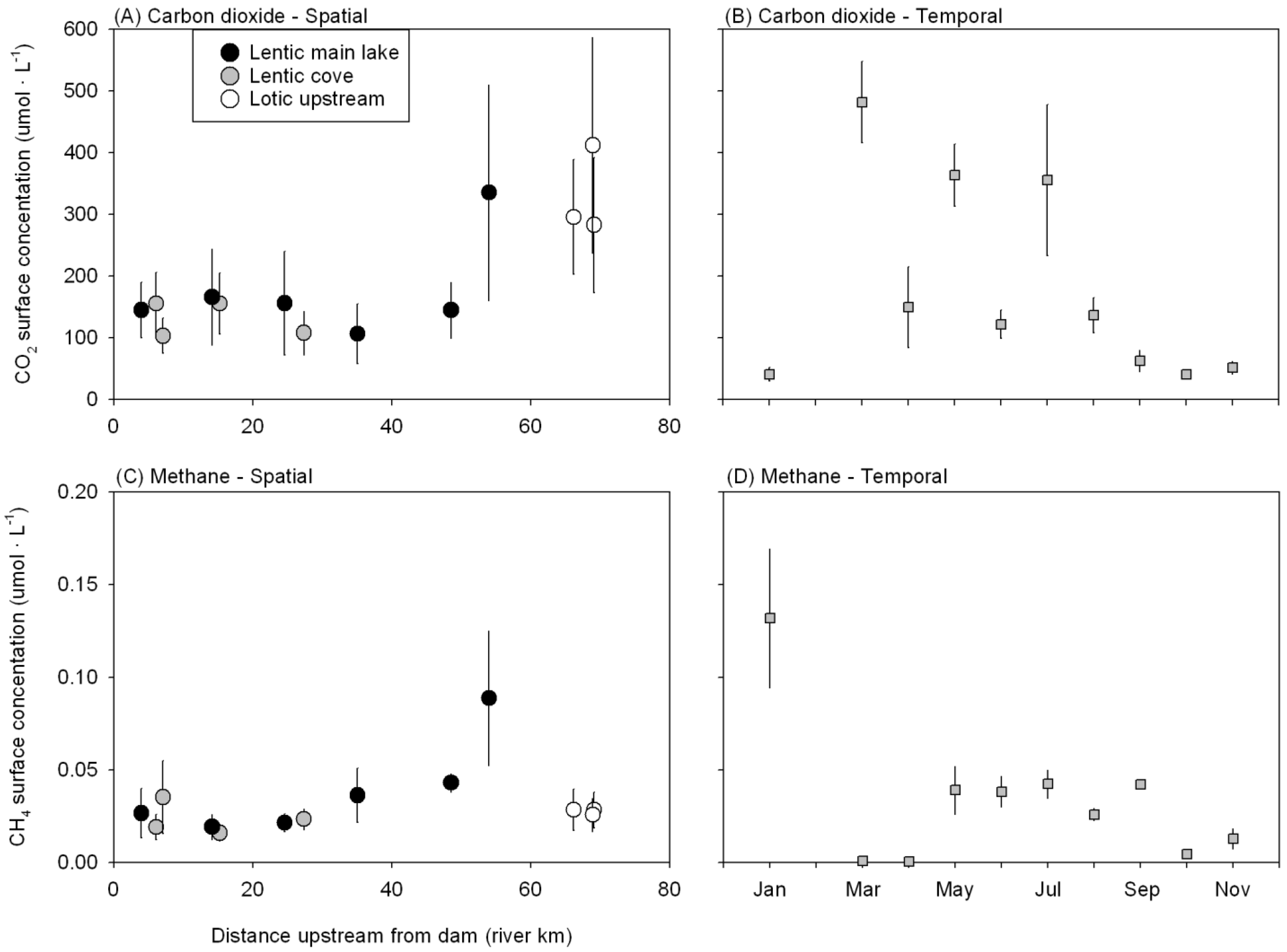
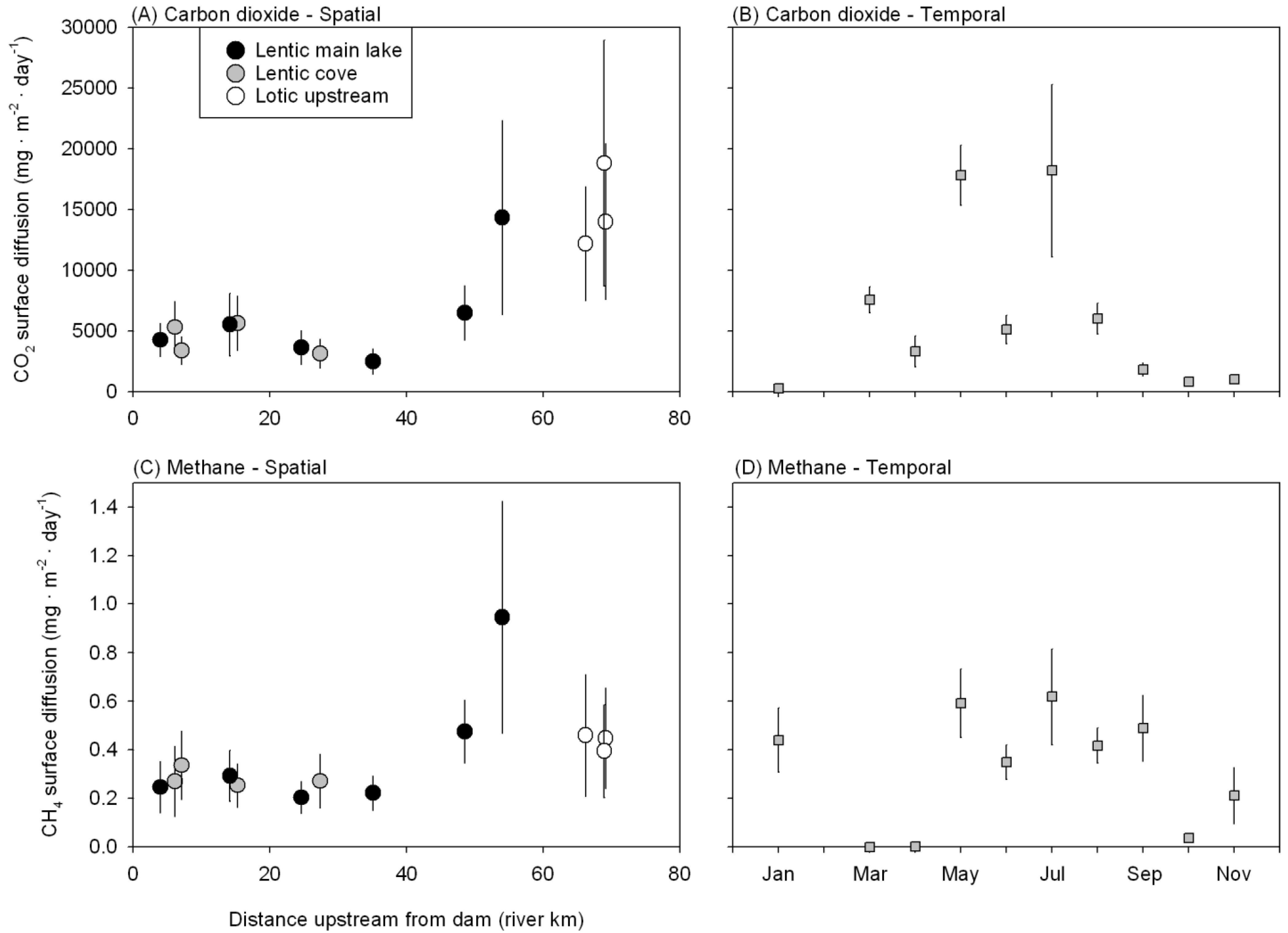
3.2. CO2 and CH4 Emissions from Douglas Lake
3.3. Modelling Spatial and Temporal Variation in GHG Emissions
4. Conclusions
Acknowledgments
Author Contributions
Conflicts of Interest
References
- Victor, D.G. Strategies for cutting carbon. Nature 1998, 395, 837–838. [Google Scholar] [CrossRef]
- Rudd, J.W.M.; Harris, R.; Kelly, C.A.; Hecky, R.E. Are hydroelectric reservoirs significant sources of greenhouse gases? AMBIO 1993, 22, 246–248. [Google Scholar]
- Beaulieu, J.J.; Smolenski, R.L.; Nietch, C.T.; Townsend-Small, A.; Elovitz, M.S. High methane emissions from a midlatitude reservoir draining an agricultural watershed. Environ. Sci. Technol. 2014, 48, 11100–11108. [Google Scholar] [CrossRef] [PubMed]
- Barros, N.; Cole, J.J.; Tranvik, L.J.; Prairie, Y.T.; Bastviken, D.; Huszar, V.L.M.; del Giorgio, P.; Roland, F. Carbon emission from hydroelectric reservoirs linked to reservoir age and latitude. Nat. Geosci. 2011, 4, 593–596. [Google Scholar] [CrossRef]
- Wetzel, R.G. Limnology: Lake and River Ecosystems, 3rd ed.; Academic Press: San Diego, CA, USA, 2001. [Google Scholar]
- Galy-Lacaux, C.; Delmas, R.; Jambert, C.; Dumestre, J.F.; Labroue, L.; Richard, S.; Gosse, P. Gaseous emissions and oxygen consumption in hydroelectric dams: A case study in French Guyana. Glob. Biogeochem. Cycles 1997, 11, 471–483. [Google Scholar] [CrossRef]
- McGinnis, D.F.; Greinert, J.; Artemov, Y.; Beaubien, S.E.; Wuest, A. Fate of rising methane bubbles in stratified waters: How much methane reaches the atmosphere? J. Geophys. Res. 2006, 111. [Google Scholar] [CrossRef] [Green Version]
- Bastviken, D.; Cole, J.J.; Pace, M.L.; van de Bogert, M.C. Fates of CH4 from different lake habitats: Connecting whole-lake budgets and CH4 emissions. J. Geophys. Res. Biogeosci. 2008, 113. [Google Scholar] [CrossRef]
- Delsontro, T.; Kunz, M.J.; Kempter, T.; Wuest, A.; Wehrli, B.; Senn, D.B. Spatial heterogeneity of methane ebullition in a large tropical reservoir. Environ. Sci. Technol. 2011, 45, 9866–9873. [Google Scholar] [CrossRef] [PubMed]
- Bogard, M.J.; del Giorgio, P.A.; Boutet, L.; Chaves, M.C.G.; Prairie, Y.T.; Merante, A.; Derry, A.M. Oxic water column methanogenesis as a major component of aquatic CH4 fluxes. Nat. Commun. 2014, 5. [Google Scholar] [CrossRef] [PubMed]
- Soumis, N.; Duchemin, E.; Canuel, R.; Lucotte, M. Greenhouse gas emissions from reservoirs of the western United States. Glob. Biogeochem. Cycles 2004, 18. [Google Scholar] [CrossRef]
- Hofmann, H. Spatiotemporal distribution patterns of dissolved methane in lakes: How accurate are the current estimations of the diffusive flux pathway? Geophys. Res. Lett. 2013, 40, 2779–2784. [Google Scholar] [CrossRef]
- Kelly, C.A.; Rudd, J.W.M.; Bodaly, R.A.; Roulet, N.P.; St. Louis, V.L.; Heyes, A.; Moore, T.R.; Schiff, S.; Aravena, R.; Scott, K.J.; et al. Increases in fluxes of greenhouse gases and methyl mercury following flooding of an experimental reservoir. Environ. Sci. Technol. 1997, 31, 1334–1344. [Google Scholar] [CrossRef]
- Kankaala, P.; Huotari, J.; Peltomaa, E.; Saloranta, T.; Ojala, A. Methanotrophic activity in relation to CH4 efflux and total heterotrophic bacterial production in a stratified, humic, boreal lake. Limnol. Oceanogr. 2006, 51, 1195–1204. [Google Scholar] [CrossRef]
- St. Louis, V.; Kelly, C.A.; Duchemin, E.; Rudd, J.W.M.; Rosenberg, D.M. Reservoir surfaces as sources of greenhouse gases to the atmosphere: A global estimate. BioScience 2000, 50, 766–775. [Google Scholar] [CrossRef]
- DelSontro, T.; McGinnis, D.F.; Sobek, S.; Ostrovsky, I.; Wehrli, B. Extreme methane emissions from a Swiss hydropower reservoir: Contribution from bubbling sediments. Environ. Sci. Technol. 2010, 44, 2419–2425. [Google Scholar] [CrossRef] [PubMed]
- Maeck, A.; del Sontro, T.; McGinnis, D.F.; Fischer, H.; Flury, S.; Schmidt, M.; Fietzek, P.; Lorke, A. Sediment trapping by dams creates methane emission hot spots. Environ. Sci. Technol. 2013, 47, 8130–8137. [Google Scholar] [CrossRef] [PubMed]
- American Public Health Association. Standard Methods for the Examination of Water and Wastewater, 21st ed.; American Public Health Association: Washington, DC, USA, 2005. [Google Scholar]
- Tennessee Valley Authority Website. Available online: http://www.tva.gov (accessed on 1 February 2015).
- UNESCO/The International Hydropower Association. GHG Measurement Guidelines for Freshwater Reservoirs; Goldenfum, J.A., Ed.; London, UK, 2010. [Google Scholar]
- Duchemin, E.; Lucotte, M.; Canuel, R. Comparison of static chamber and thin boundary layer equation methods for measuring greenhouse gas emissions from large water bodies. Environ. Sci. Technol. 1999, 33, 350–357. [Google Scholar] [CrossRef]
- Demarty, M.; Bastien, J.; Tremblay, A.; Hesslein, R.; Gill, R. Greenhouse gas emissions from boreal reservoirs in Manitoba and Quebec, Canada, measured with automated systems. Environ. Sci. Technol. 2009, 43, 8908–8915. [Google Scholar] [CrossRef] [PubMed]
- Ioffe, B.V.; Vitenberg, A.G. Head-Space Analysis and Related Methods in Gas Chromotography; Wiley: New York, NY, USA, 1984. [Google Scholar]
- National Oceanic and Atmospheric Administration Website. Available online: http://www. noaa.gov (accessed on 1 February 2015).
- Stocker, T.F.; Qin, D.; Plattner, G.K.; Tignor, M.; Allen, S.K.; Boschung, J.; Nauels, A.; Xia, Y.; Bex, V.; Midgley, P.M. (Eds.) Intergovernmental Panel on Climate Change. Summary for Policymakers. In Climate Change 2013: The Physical Science Basis; Contribution of Working Group I to the Fifth Assessment Report of the Intergovernmental Panel on Climate Change; Cambridge University Press: Cambridge, UK; New York, NY, USA, 2013.
- Cutler, D.R.; Edwards, T.C.; Beard, K.H.; Cutler, A.; Hess, K.T.; Gibson, J.; Lawler, J.J. Random forests for classification in ecology. Ecology 2007, 88, 2783–2792. [Google Scholar] [CrossRef] [PubMed]
- Breiman, L.; Cutler, A. Random Forests. Available online: https://www.stat.berkeley.edu/~breiman/RandomForests/cc_home.htm (accessed on 2 April 2014).
- Tremblay, A.; Lambert, M.; Gagnon, L. Do hydroelectric reservoirs emit greenhouse gases? Environ. Manag. 2004, 33, S509–S517. [Google Scholar] [CrossRef]
- Teodoru, C.R.; Prairie, Y.T.; del Giorgio, P.A. Spatial heterogeneity of surface CO2 fluxes in a newly created Eastmain-1 Reservoir in Northern Quebec, Canada. Ecosystems 2011, 14, 28–46. [Google Scholar] [CrossRef]
- Tadonléké, R.D.; Marty, J.; Planas, D. Assessing factors underlying variation of CO2 emissions in boreal lakes vs. reservoirs. FEMS Microb. Ecol. 2012, 79, 282–297. [Google Scholar] [CrossRef]
- Huttunen, J.T.; Alm, J.; Liikanen, A.; Juutinen, S.; Larmola, T.; Hammar, T.; Silvola, J.; Martikainen, P.J. Fluxes of methane, carbon dioxide and nitrous oxide in boreal lakes and potential anthropogenic effects on the aquatic greenhouse gas emissions. Chemosphere 2003, 52, 609–621. [Google Scholar] [CrossRef]
- Kemenes, A.; Forsberg, B.R.; Melack, J.M. CO2 emissions from a tropical hydroelectric reservoir (Balbina, Brazil). J. Geophys. Res. 2011, 116. [Google Scholar] [CrossRef]
- Jacinthe, P.A.; Filippelli, G.M.; Tedesco, L.P.; Raftis, R. Carbon storage and greenhouse gases emission from a fluvial reservoir in an agricultural landscape. Catena 2012, 94, 53–63. [Google Scholar] [CrossRef]
- Hertwich, E.G. Addressing Biogenic Greenhouse Gas Emissions from Hydropower in LCA. Environ. Sci. Technol. 2013, 47, 9604–9611. [Google Scholar] [CrossRef] [PubMed]
- West, W.E.; Coloso, J.J.; Jones, S.E. Effects of algal and terrestrial carbon on methane production rate and methanogen community structure in a temperature lake sediment. Freshw. Biol. 2012, 57, 949–955. [Google Scholar] [CrossRef]
- Guisan, A.; Thuiller, W. Predicting species distributions: Offering more than simple habitat models. Ecol. Lett. 2005, 8, 993–1009. [Google Scholar] [CrossRef]
- Tilman, D.; Fargione, J.; Wolff, B.; D’Antonio, C.; Dobson, A.; Howarth, R.; Schindler, D.; Schlesinger, W.J.; Simberloff, D.; Swackhamer, D. Forecasting agriculturally driven global environmental change. Science 2001, 292, 281–284. [Google Scholar] [CrossRef] [PubMed]
- Podgrajsek, E.; Sahlee, E.; Rutgersson, A. Diurnal cycle of lake methane flux. J. Geophys. Res. Biogeosci. 2014, 119, 236–248. [Google Scholar] [CrossRef]
- Grossart, H.P.; Frindte, K.; Dziallas, C.; Eckert, W.; Tang, K.W. Microbial methane production in oxygenated water column of an oligotrophic lake. Proc. Natl. Acad. Sci. USA 2011, 108, 19657–19661. [Google Scholar] [CrossRef] [PubMed]
- Tranvik, L.J.; Downing, J.A.; Cotner, J.B.; Loiselle, S.A.; Striegl, R.G.; Ballatore, T.J.; Dillon, P.; Finlay, K.; Fortino, K.; Knoll, L.B.; et al. Lakes and reservoirs as regulators of carbon cycling and climate. Limnol. Oceanogr. 2009, 54, 2298–2314. [Google Scholar] [CrossRef]
- Intergovernmental Panel on Climate Change. IPCC Special Report on Renewable Energy Sources and Climate Change Mitigation; Contribution of Working Group III to the Fifth Assessment Report of the Intergovernmental Panel on Climate Change; Edenhofer, O., Pichs-Madruga, R., Sokona, Y., Seyboth, K., Matschoss, P., Kadner, S., Zwickel, T., Eickemeier, P., Hansen, G., Schlömer, S., et al., Eds.; Cambridge University Press: Cambridge, UK; New York, NY, USA, 2013; p. 1075. [Google Scholar]
- Chang, X.; Liu, X.; Zhou, W. Hydropower in China at present and its further development. Energy 2010, 35, 4400–4406. [Google Scholar] [CrossRef]
- McManamay, R.A.; Samu, N.; Kao, S.C.; Bevelhimer, M.S.; Hetrick, S.C. A multi-scale spatial approach to address environmental effects of small hydropower development. Environ. Manag. 2014, 55, 217–243. [Google Scholar] [CrossRef] [PubMed]
- Mekong River Commission. Economic, Environmental and Social Impact Assessment of Basin-Wide Water Resources Development Scenarios; Mekong River Commission: Vientiane, Laos, 2009. [Google Scholar]
- Hydropower Policy; Ministry of Power, Government of India (GOI): New Delhi, India, 2008.
- Hadjerioua, B.Y.; Wei, Y.; Kao, S.C. An Assessment of Energy Potential at Non-Powered Dams in the United States; GPO DOE/EE-0711; Wind and Water Power Program, Department of Energy: Washington, DC, USA, 2012. [Google Scholar]
- Kao, S.C.; McManamay, R.A.; Stewart, K.M.; Samu, N.M.; Hadjerioua, B.; DeNeale, S.T.; Yeasmin, D.; Pasha, M.F.K.; Oubeidillah, A.A.; Smith, B.T. New Stream-Reach Development: A Comprehensive Assessment of Hydropower Energy Potential in the United States; GPO DOE/EE-1063; Wind and Water Power Program, Department of Energy: Washington, DC, USA, 2014. [Google Scholar]
- Canadian Hydropower Association. Report of Activities. Available online: http:// canadahydro.ca/reportsreference/cha-reports-and-publications (accessed on 1 February 2015).
- Hydropower in Canada: Past Present and Future. Available online: http://canadahydro.ca/reportsreference/cha-reports-and-publications (accessed on 1 February 2015).
© 2015 by the authors; licensee MDPI, Basel, Switzerland. This article is an open access article distributed under the terms and conditions of the Creative Commons Attribution license (http://creativecommons.org/licenses/by/4.0/).
Share and Cite
Mosher, J.J.; Fortner, A.M.; Phillips, J.R.; Bevelhimer, M.S.; Stewart, A.J.; Troia, M.J. Spatial and Temporal Correlates of Greenhouse Gas Diffusion from a Hydropower Reservoir in the Southern United States. Water 2015, 7, 5910-5927. https://doi.org/10.3390/w7115910
Mosher JJ, Fortner AM, Phillips JR, Bevelhimer MS, Stewart AJ, Troia MJ. Spatial and Temporal Correlates of Greenhouse Gas Diffusion from a Hydropower Reservoir in the Southern United States. Water. 2015; 7(11):5910-5927. https://doi.org/10.3390/w7115910
Chicago/Turabian StyleMosher, Jennifer J., Allison M. Fortner, Jana R. Phillips, Mark S. Bevelhimer, Arthur J. Stewart, and Matthew J. Troia. 2015. "Spatial and Temporal Correlates of Greenhouse Gas Diffusion from a Hydropower Reservoir in the Southern United States" Water 7, no. 11: 5910-5927. https://doi.org/10.3390/w7115910