Article

Lagrangian Cloud Tracking and the Precipitation-Column Humidity Relationship

Department of Land, Air and Water Resources, University of California Davis, Davis, CA 95616, USA
Atmosphere 2018, 9(8), 289; https://doi.org/10.3390/atmos9080289
Submission received: 5 June 2018 / Revised: 11 July 2018 / Accepted: 19 July 2018 / Published: 26 July 2018
(This article belongs to the Special Issue Precipitation: Measurement and Modeling)

Abstract

:
The tropical, oceanic mean relationship between column relative humidity and precipitation is highly non-linear. Mean precipitation remains weak until it rapidly picks up and grows at high column humidity. To investigate the origin of this relationship, a Lagrangian cloud tracking code, RAMStracks, is developed, which can follow the evolution of clouds. RAMStracks can record the morphological properties of convective clouds, the meteorological environment of clouds, and their effects. RAMStracks is applied to a large-domain radiative convective equilibrium simulation, which produces a complex population of convective clouds. RAMStracks records the lifecycle of 501 clouds through growth, splits, mergers, and decay. The mean evolution of all these clouds is examined. It is shown that the column humidity evolves non-monotonically, but that lower-level and upper-level contributions to total moisture do evolve monotonically. The precipitation efficiency of tropical storms tends to increase with cloud age. This is confirmed using a prototype testing method. The same method reveals that different tracked clouds with similar initial conditions evolve in very different ways. This makes drawing general conclusions from individual storms difficult. Finally, the causality of the precipitation-column humidity relationship is examined. A Granger Causality test, as well as regressions, suggest that moisture and precipitation are causally linked, but that the direction of causality is ambiguous. Much of this link appears to come from the lower-level moisture’s contribution to column humidity.

1. Introduction

In the moist tropics, clear air is often observed to give way to shallow clouds, which grow vertically, and then slowly decay through a stratiform phase [1]. This evolution describes not only the lifetime of some isolated clouds, but also that of the population of convection at larger time and space scales during a mesoscale convective event or during the Madden Julian Oscillation. Mapes et al. [2] pointed out the ubiquity of this canonical evolution. Broadly, the evolution arises from the action of convection on the atmosphere in which it exists. Clouds locally enhance the moisture content of the atmosphere through horizontal or vertical flux convergence, which allows for further convective growth, while detrainment into dry air and condensation within the cloud coincidentally deplete in-cloud and net moisture, respectively, and allow for decay. As such, the lifetime of a tropical convective cloud is marked by a competition between processes that moisten and processes that dry, and, more broadly, processes that favor cloud growth and cloud decay. Eventually, it seems, decay processes inevitably overcome growth processes.
While it is possible to understand the large-scale Eulerian moisture tendency of the population of convection through stationary sounding networks [3], it is difficult to characterize the effect an individual cloud has on the atmospheric moisture field without a Lagrangian perspective. Tracking individual clouds or cloud systems from model, radar, and satellite data has a long history, but its potential is only now coming to be in widespread use. Tracking clouds from satellite data is perhaps the most common method for examining the cloud lifecycle and its effects. From consecutive snapshots from geostationary data, individual clouds can be observed to grow (widen) or decay (narrow) [4,5,6]. Such methods have been used successfully to investigate the growth and decay of storms all over the world [7,8], and have the advantage of observing a natural distribution of clouds. Using sequential ground-based radar volumes can add a vertical component to tracked clouds [9,10]. However, radars may have difficulty observing clouds before they begin to precipitate and may only observe a cloud once every few minutes. Thus, neither can capture the lifetime of all possible target clouds. To remedy this problem, clouds can be tracked in a cloud resolving model [11,12,13,14,15]. The problem with this method is that the computational expense of executing a model over which a reliable tracking code can be run offline is very high (see Methods) and the complexity and finality of running one online is daunting. Tracking clouds in a model is also limited by the realism of the model and the imagination of the user. However, tracking clouds in a model has the advantage of allowing environmental and cloud properties to be tracked fully in four dimensions. This is the method that will be employed below.
Four-dimensional cloud tracking will be applied to a simulation of a tropical convective population in RAMS (Regional Atmospheric Modeling System). In so doing, we seek to address two outstanding issues facing tropical meteorology.
(1)
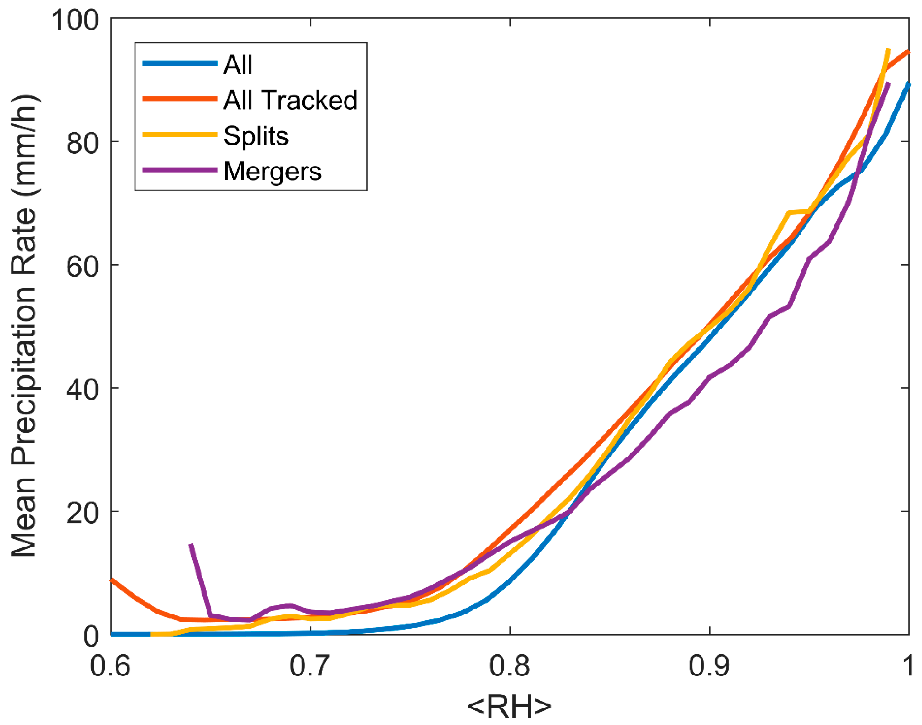
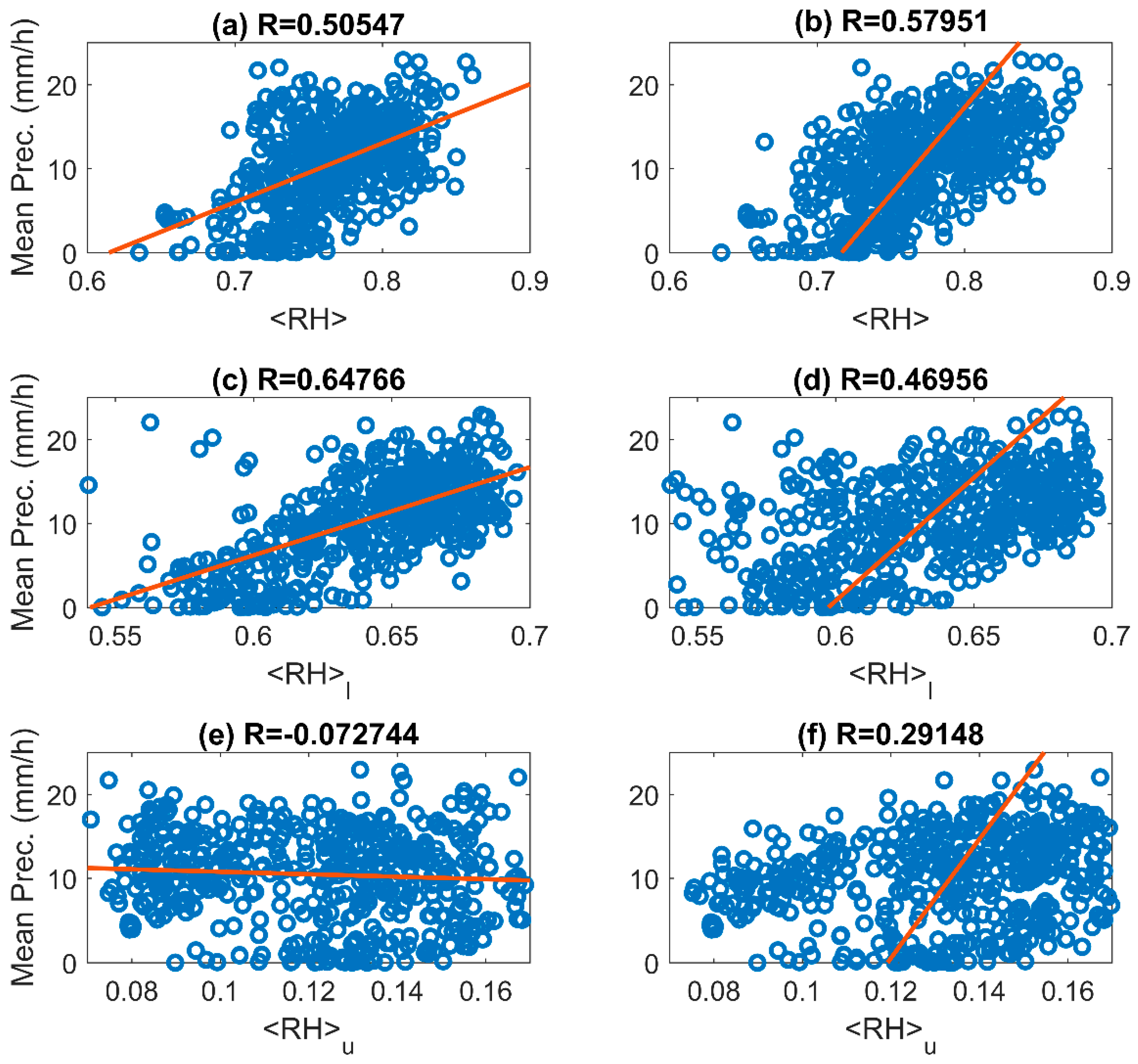
Bretherton et al. [16] pointed out a remarkable behavior, whereby the mean precipitation rate grows rapidly above some threshold value in saturation-normalized, vertically integrated water vapor content (referred to as <RH>, for column relative humidity, in what follows). Figure 1 illustrates this behavior in the simulation described below. Many studies have examined this behavior and attempted to explain its origins or consequences [17,18,19,20,21,22,23,24]. Several of these studies examine composite-event time series in an effort to infer causality in the precipitation-<RH> relationship (shortened to P(<RH>) for convenience) [23,25,26]. What is lacking, though, is a description of the causality based on individual events, which as we will show, can behave very differently than composite timeseries. By perturbing a model’s entrainment rate, Kuo et al. [26] argue that the form of P(<RH>) can only be reproduced when moisture leads precipitation. However, it could just as well be argued that since gravitationally settling precipitation often evaporates as it falls, higher precipitation rate columns moisten their local environment such that the intensity of precipitation affects moisture content. Kuo et al. [26] alter the re-evaporation of precipitation in their model and see little change in P(<RH>), but the limitedness of sensitivity could be due to the simplicity of such a scheme in a model with parameterized convection. Thus, previous work suggests in a coarse way that moister atmospheres precipitate more, rather than vice versa. This largely agrees with intuition. However, this conclusion needs to be examined at the cloud scale on short timescales. If causality can be determined, this simple relationship could be used to make physically-based precipitation or moisture forecasts.
(2)
Variability in the evolution among clouds is often necessarily ignored in order to try to draw generalizable conclusions. Clouds and cloud systems are broadly imagined progressing in a systematic way from shallow, to deep, to stratiform (as above). For example, Igel [27] contextualized P(<RH>) as a function of this evolution, but that study failed to explain complex cloud evolutions which are known to exist. It is obvious from everyday experience that many clouds do not follow a simple, scripted lifecycle. Many isolated clouds are the result of splits from larger clouds or the merger of two smaller clouds at some previous time [28,29,30,31]. These types of complex evolutions lack a sufficient conceptual place within the standard evolutionary pathway. Because variability is often ignored, it is not well understood whether complex cloud histories interact with their thermodynamic or dynamic environment uniquely. To form a more complete picture of P(<RH>), the contribution by all clouds must be accounted for.
Using a high-resolution cloud resolving model and a new cloud tracking algorithm, both the ensemble characteristics of cloud lifecycle evolutions and the temporal evolution of the precipitation-column moisture relationship and its variability are investigated below. The goal of this paper is to use cloud tracking to better characterize the complexity of the lifecycle of tropical convection and to use that to better address Points (1) and (2) in the preceding paragraph.
This paper will proceed as follows. First, the model employed and the simulation analyzed are discussed. Then, we include details of the new 4-dimensional cloud tracking algorithm, RAMStracks. Results include characterizations of normalized convective evolutions, properties of cloud splits and mergers, and causality of P(<RH>). Finally, some conclusions and discussion are offered.

2. Experiments

A more complete description of the simulation analyzed and the model used to conduct it is included in Igel et al. [24] and Igel [27]. To achieve a large statistical sample of tropical deep convective clouds, a radiative convective equilibrium simulation was conducted. The idealized simulation domain was 2000 km × 400 km at 1 km grid spacing in the horizontal with doubly-periodic lateral boundary conditions. Sixty-five stretched vertical levels were used. Convective systems are explicitly simulated. The model was run for 61 days with a diurnal cycle in incoming shortwave radiation and a fixed-temperature sea surface of 301 K. Over the course of the initial 30 days of the simulation, convective clouds begin to move through their lifecycle and eventually aggregate into two quasi-permanent moist regions spaced approximately 1000 km apart.
The Regional Atmospheric Modeling System (RAMS) [32] was used to conduct the simulation. RAMS has an advanced bin-emulating, double moment bulk microphysics scheme [33,34,35,36] that includes 8 (3 liquid and 5 ice) hydrometeor species. The fully interactive 2-stream radiation scheme of Harrington [37] was used for the simulation.

2.1. Layer Moisture

In Igel [27], we suggested that the way <RH> leads to precipitation is derived from two contributing components. The first is the contribution to total <RH> by moisture located between the sea surface and the base of the melting layer at 4 km. This was termed the lower-layer column humidity (<RH>l). <RH>l can contribute up to ~70% of total <RH>. The second component was moisture above the base of the melting layer up to the top of the atmosphere, termed <RH>u. The sum of <RH>l and <RH>u is <RH>. While <RH>u contributes up to ~30% of <RH>, it was shown that its contribution is more consequential to precipitation than an equivalent contribution from <RH>l. Like <RH> exhibits a pickup in mean precipitation at <RH> = 0.77, so too does precipitation at layer moisture quantities exhibit pickup values of <RH>l = 0.63 and <RH>u = 0.14. At layer-<RH> above these values, precipitation rapidly increases from zero. Locations with layer-<RH> above these pickup values are outlined in Figure 2 from hour 1428 of the simulation. For the full context of this figure, see Figure 3 of Igel et al. [24].

2.2. Cloud Tracking

As noted above, we are not the first to track clouds. Many others have tracked clouds in models [11,12,13,28], from radar data [9,10], or from photography [38]. Most of these previously employed methods share computational and conceptual characteristics with one another and with the method we discuss below. Therefore, the description of the new tracker is intentionally terse and limited to specifics that may not be general. The tracker discussed below is dubbed RAMStracks. The author has made it freely available.

2.3. RAMStracks

In order to track clouds in four dimensions, output from the final three days of the simulation was archived every 5 min (as in [39]). High-resolution temporal output is required to accurately link-in-time rapidly evolving clouds. While it is possible to avoid the need for finely spaced temporal output by using an online tracking method [28], offline tracking presents several benefits such as adaptability and simplicity. For the purposes of tracking, clouds are defined to be made up of two parts, “cores” and “shells”. “Cores” are defined objectively as contiguous regions of total condensate mixing ratio greater than 10−3 kg/kg; “shells” are regions above 10−4 kg/kg. As such, “cores” and “shells” should not be confused with their more frequent meanings, which carry some state or dynamic (buoyancy or vertical velocity) implications. Because convection aggregates [40,41] in radiative convective equilibrium simulations such as these, a single shell may include multiple cores. The temporal domain-average percent of rain falling at surface pixels below cores is 78% and below shells is more than 99%. Cores contribute 88% of all rain falling at >1 mm h−1. Splitting clouds into pieces in order to focus the tracker on the most important part of a cloud was inspired by the methods of Dawe and Austin [13], who refer to cloud pieces as “cloudlets” and by Futyan and Del Genio [4] who use “detect and spread”, which uses multiple thresholds to begin and end a search for contiguous regions.
RAMStracks was developed to track individual cores backward in time. This ultimately arbitrary choice has the benefit of allowing the tracker to initialize a new object by identifying robustly developed cloud structures at the end of their lifetime. While it is not done here, backward tracking also has the potential to track entities back toward their genesis, where they are often poorly developed and difficult to identify objectively by successively relaxing (size or intensity) thresholds. Therefore, backward tracking is implemented as a future-proof method. We should also mention that tracking air backward is not in itself novel. For clarity, we will discuss the cloud tracker as though it tracked forward in time. For everything we discuss below, forward and backward tracking would result in identical results. RAMStracks begins by identifying cloud cores at some time, TN. This is done in three dimensions such that cores are contiguous volumes of cloudy air meeting the core threshold of at least 200 model grid volumes. This is an arbitrary threshold that is necessary to prevent numerous small cumulus clouds from being tracked; such size thresholds are often employed [12,42]. Small clouds are not the focus of this work, but RAMStracks could be adapted trivially to include them in the future. A total pixel number threshold was chosen, rather than, say, limits on morphology as used to parse observational data in Igel et al. [43], so as to more easily track deep convection across its entire lifecycle which includes periods of significant differences in morphology. Because RAMS is set up with a stretched vertical grid, 200 grid volumes represent a smaller physical volume near the surface than aloft. This aids in tracking cores early in their lifetime, when they are physically smaller. The smallest object tracked is just 4 km wide at its genesis in the tracker, but has a maximum width of 70 km. All cores are given a unique identification number (CloudID). Environmental and cloud process data are recorded for cloudy pixels (see next). Shells are then identified. A shell volume completely enclosing a core volume is then linked to that core and its information becomes shell information for that core. Any shells that do not enclose a core are discarded. A tracked core that exists for a single or across multiple archive time steps will be referred to as a “cloud object” in what follows. “Shells” will not be discussed below for brevity and for clarity, but we wish to note them as a special capability of RAMStracks.
Once clouds at TN are successfully identified, we use the model wind to predict the cloud’s position at some future time in the simulation, TN+1, by using the wind to “advect” the cloud. At TN+1, the exact same process of identifying cores and shells is conducted. We assume that newly identified clouds that overlap with an advected cloud by at least 10% of their respective pixels and whose centers are less than 10 km apart are later realizations of the same cloud. If no projected TN cloud meets these thresholds, the TN+1 cloud is assumed to be a new cloud at the beginning of its lifetime. Any TN cloud that does not project onto a TN+1 cloud is assumed to have died at TN. Its CloudID is then retired.
Splits of cores are handled simply. If two clouds at TN+1 meet the temporal-linking criteria for a forward-projected TN cloud object, then these clouds are assumed to have split sometime between TN and TN+1. One of the clouds retains the CloudID of the parent cloud and receives a ChildID which is identical to the CloudID of the other cloud. Mergers are handled in a similar, but logically reversed, manner with one cloud whose identity “ends” at TN+1 receiving a ParentID. Coincidentally, Heiblum et al. [14] recently used similar nomenclature and techniques for handling splits and mergers.
Objects whose centroid location comes within 10 km of any lateral boundary are flagged. This is significantly more computationally efficient than trying to track clouds across boundaries and should not bias the data when these objects are excluded from analysis, although, we note no consequential difference in results when these objects are included due to their relative infrequence in the very large domain.
A vertical shadow-projection onto the surface is made for both cores and shells. For the X-Y locations of the shadow projection, environmental and rainfall information is recorded. The quantities recorded are listed in Table 1. Shape information and a centroid location are also recorded for these shadow pixels. These quantities are also listed in Table 1. Most quantities should be self-explanatory. The measurement listed as “flux” is the moisture mass flux for shadow projection columns integrated vertically from 1 km to 14 km. The units of flux are mm h−1 so the quantity can be compared meaningfully with rain rates. Thus, this quantity is somewhat analogous to precipitation, but a positive value indicates vapor moving upward instead of raindrops falling downward. If, in convective updrafts all water mass were to instantaneously condense and fall to the surface, the flux would equal precipitation. “Shear” is a bulk difference between mean lower layer wind (1–2 km AGL) and upper level wind (10–15 km AGL), similar to that used in Igel and van den Heever [44]. Quantities in Table 1 with sizes of t × n will often be averaged over the cloud’s spatial extent. This averaging results in an effective size of t × 1. Averaging the data in this way makes interpretation of data easy, but limits some of the novelty of tracking.
Across the 72 h of trackable model output, 501 clouds are tracked (i.e., 501 CloudIDs are assigned). From these, clouds that exist at the initial or final time step are ignored leaving 487. A simple attempt at identifying the structural characteristics of the clouds is made (Table 1: Type) following the thresholds identified in Igel [27]. Precipitation (P), <RH>l, and <RH>u are examined across the lifetime of the object. Clouds with continuously low <RH>u (<0.12) and low P (<30 mm h−1) are assigned to the “shallow” category. Clouds with low <RH>l (<0.62) and high P (>7 mm h−1) across their lifetime are assigned to the “stratiform” category. Clouds with low <RH>l and low to zero P are assigned to the “anvil” category. About half, 249, of clouds fall in the “deep convection” category, which requires high <RH>l (>0.62) and <RH>u (>0.12). Deep convective clouds are essentially anything that is not filtered into another category. The tracker spends most of its time concerned with deep convection, as deep objects are numerous and, often, long-lived. The centroid locations across the lifetimes of clouds present at hour 1428 are traced in Figure 2.

3. Results

3.1. Normalization

To begin to understand RAMStracks clouds, a convenient way to characterize the evolution of many clouds simultaneously is needed. This can be done in two different but complementary ways with RAMStracks data. The first is by projecting the lifetime of every cloud onto a homogeneous time grid. This method treats the cloud lifetime as the master clock. Cloud genesis occurs at time zero and cloud death occurs at time one. This method is useful if the evolution of clouds follows a simple script. The cloud-clock method has been used frequently in the past [4,39,45,46]. The second method is one that assumes that the wall-clock is the master clock. In this method, physical processes are assumed to occur at defined rates as measured by some universal clock. The wall-clock has been used frequently for tracked clouds and updrafts [7,12,39,47] and for compositing [2,48,49]. Both normalizations can be used to provide interesting insights into the lifecycle of clouds and the link between <RH> and P, but we will focus on the cloud-clock normalization.
The cloud-clock method we develop is applied to clouds that exist for at least 20 min (5 archive steps). Properties of these clouds are projected onto a grid of time-length 5 via a shape-preserving spline interpolation downscaling. For example, a cloud that is 5 output steps long would remain unchanged by the normalization, while a cloud that is 20 output steps long would (effectively) see its first through fourth output steps averaged onto the first leg of the cloud-clock time grid, its fifth through ninth onto the second, and so on. A spline interpolation downscaling ensures that all clouds of at least 5 output steps are treated equally, regardless of their integer divisibility by 5. Therefore, the input to our averaging routine is a vector of cloud properties that is 5 times steps long or longer and the output is a vector of properties that is exactly 5 time units long. 246 clouds contribute to the composites. Of those, 57% have lifetimes longer than an hour.
Figure 3 shows the result of the cloud-clock normalization for a variety of important environmental characteristics and Lagrangian cloud properties. Over the average lifetime of a cloud (blue line), Figure 3a shows that <RH> begins just above the mean pickup value at <0.77>, rapidly increases, and then gradually decreases down toward the pickup value. Precipitation (Figure 3d) broadly follows the same pattern. We should note that Figure 1 shows that tracked clouds exhibit a somewhat lower <RH> pickup value thanks to the high threshold used to define clouds. If this is taken into account, then clouds actually initiate well above the pickup value. <RH>l falls over the lifetime of the prototype cloud. It begins above the threshold in <RH>l and decreases toward the threshold. <RH>u increases over the prototype lifetime and increases toward the upper layer threshold. This prototype evolution illustrates how clouds redistribute moisture vertically (i.e., release potential instability) while simultaneously generating surface precipitation. This confirms the simplest views of the role of convection [50] in RCE. Because P tends to evolve more slowly than <RH> in Figure 3, the P(<RH>) is not quite immutable over the lifetime of clouds but traces out a pattern similar to those seen in Masunaga [51] whereby as <RH> increases, P is systematically lower than when <RH> decreases. Igel [27] hints that these traces are due to effectively very different contributions to rainfall generation from <RH>l and <RH>u.
The other interesting result from Figure 3a is that while <RH> is lower at the end of the cloud prototype lifetime than at the beginning, it is not markedly so. This implies that clouds dry the atmosphere, but not significantly, which is somewhat counterintuitive, given that clouds are the only mechanism that effectively reduces atmospheric moisture in the net. Insignificant drying [52] or even moistening [53] has been seen before in composite lifetimes. While the moisture state of clouds may not change much between the beginning and end of a cloud’s lifetime, the large-scale atmosphere is losing moisture from heavy precipitation. This means clouds are actively drying the adjacent clear air, which is feeding moisture into the clouds to produce precipitation while clouds themselves remain moist.
Figure 3 shows many additional prototype evolutions of cloud properties. The precipitation efficiency (PE) of convection (Figure 3f), calculated as P divided by the vertically integrated moisture flux (Figure 3e), broadly increases with prototype age. Thus, one might loosely define a (heavily precipitating) cloud object as an entity with broadly increasing PE. This makes some sense from two perspectives. As microphysical populations age and updrafts weaken, precipitation will inevitably become more intense (and therefore by assertion, more efficient). However, from a more holistic standpoint, the lifecycle of anything must evolve from generating life (i.e., cloud) to destroying it. In this sense, it is inevitable that PE will increase as cloud objects transition from growth to decay. If PE did not increase, clouds would grow and moisten the atmosphere forever.
In Igel et al. [24], it was shown that column-integrated warm rain production and melting were both important statistical predictors of P. The evolutions of these are shown in Figure 3g,h. These evolutions resemble <RH>l and <RH>u, respectively, but they are not redundant. The evolution of precipitation is similar to the evolution of warm rain (Figure 3g) with the exception of the stratiform cloud. This helps to confirm the importance of processes occurring in the lower levels of the cloud to total precipitation. Melting (Figure 3h) is highest for stratiform clouds and appears to account for much of the shape of the evolution of precipitation. Melting tends to increase with time in deep clouds as they age. Shallow clouds exhibit almost no melting.
The fractal dimension is defined as the ratio of the perimeter of an object to the perimeter its area would have if it were a perfect circle. It is a measure of the “jaggedness” of the perimeter of an enclosed area. A more jagged-edged area has a higher fractal dimension. Assessments of fractal dimensions have been used to assess cloud processes [54,55] and objectively identify cloud types [56] from satellite data. Here, fractal dimension is found using regression of the population of clouds at each normalized time interval following Batista-Tomás [56] to improve robustness. The evolution of fractal dimension of the shadow projection (Figure 3k) shows that clouds begin life as a rough patch of clouds, organize into a more circular mass as they mature, and then become more irregular as they decay. This evolution could have important implications for entrainment. A higher fractal dimension cloud has a larger perimeter for every unit of area that that perimeter encloses, so entrainment per unit area might also be higher. This would imply that the deep convective lateral bulk entrainment rate would evolve nonmonotonically over the lifetime of a cloud as the fractal properties of the cloud evolve. The fractal dimension of shallow convection (see next) decreases with time as the cloud system organizes but is very high throughout cloud lifetime. This might result in very high stochastic detrainment per unit area which would allow shallow clouds to efficiently moisten the atmosphere [57].
Next, we use the RAMSTracks cloud type assessment to examine the prototype evolution of different “types” of clouds. Across Figure 3, results that include all clouds are broadly similar to results for just deep convective objects. This seems to be both a consequence of statistics, as deep convection makes up 50% of all objects, and physics, as the combination of shallow and stratiform clouds often resembles the effect of deep clouds. Shallow and stratiform clouds, however, often behave very differently than deep convective clouds or than each other. Both P and <RH> evolve nearly monotonically in these two cloud types. Both increase with time in shallow clouds, and both primarily decrease in stratiform clouds. This broadly confirms the conceptual roles of these clouds discussed in Igel [27] and elsewhere. Over their prototype lifetime, shallow clouds increase both their <RH>l and <RH>u. While <RH>l is always above the lower-layer threshold value, <RH>u never nears its layer threshold value. This indicates that clouds that remain shallow throughout their lifetime fail to moisten the upper layer sufficiently to grow vertically. The stratiform prototype begins its life with <RH>u just above the layer threshold and ends life with <RH>u only marginally below it. The more significant change during the lifetime of stratiform clouds is in <RH>l which drops to well below the lower-layer threshold. This indicates that low-level drying from stratiform downdrafts is more significant than moistening from evaporation of raindrops. <RH> in stratiform clouds decreases as a result (Figure 3a). Also noteworthy is that every cloud type always has (mean) positive moisture flux (Figure 3e) and that stratiform clouds cease to exist when their moisture flux approaches zero. Stratiform clouds also exhibit systematically higher PE than any other cloud type and are capable of drying cloudy columns through precipitation alone.
For the mean of all clouds and for each cloud type separately, the lateral speed of motion (Figure 3i) of the cloud centroid changes with lifecycle stage. Initially, speeds remain nearly constant or decrease slightly. Then, speeds increase toward the end of the prototype. The final centroid velocity is a convolution of two effects: actual motion of a storm and growth and decay of cloud mass at the cloud’s edge. This dependence on lifetime of the speed of translation of clouds is the fundamental reason a Lagrangian tracking method is useful. In an Eulerian framework, relatively fast-moving clouds are sampled differently than slower ones, which violates the frozen turbulence hypothesis [58]—a necessary assumption in order to equate Eulerian and Lagrangian results.
Bulk vertical wind shear (Figure 3k) is highest for stratiform clouds and lowest for shallow clouds. It tends to fall over the lifetime of the former and rise during that of the latter. One possible interpretation, among many, of these evolutions is that stratiform clouds decay as their supportive shear slackens and that shallow clouds that fail to grow vertically progressively lose local moisture due to its being advected away from the clouds by vertically sheared flows.

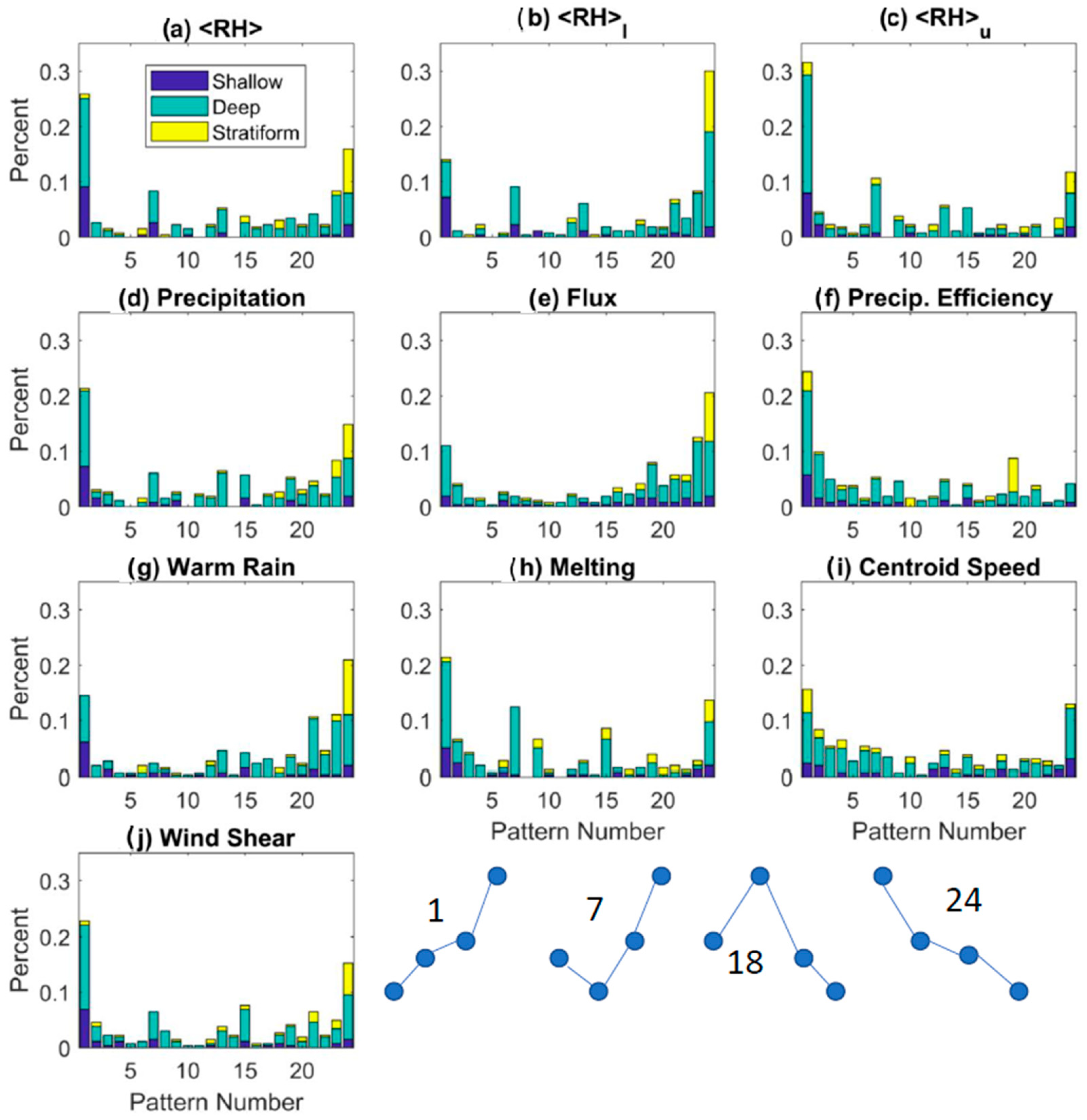
3.2. Pattern Fitting

In order to test whether the normalized cloud evolutions are actually reflective of patterns occurring in individual clouds, the permutation spectrum test of Kulp and Zunino [59] is modified and applied. The permutation spectrum test sorts time series data into patterns based on temporal evolution. The relative population of some evolutionary patterns to others is used to imply the level of physical (chaotic) determinism compared to the level of stochasticism. Here, it will be applied to understand the degree of determinism in the evolution of cloud properties and to check whether the normalized evolutions represent common patterns or whether they are an alias of two or more common patterns.
For the permutation spectrum test [59], all possible sequential evolutions of an environmental variable, for example <RH>, are represented by a particular pattern number. Pattern 1 is a monotonic increase in <RH> over the normalized lifetime of the cloud (of 4 units length (while prototypes in Figure 3 have a length of 5, 4 nodes were used here to limit the number of ordinal patterns which goes as the factorial of the length in order to achieve some statistical power with 487 clouds)) (see Figure 4). Pattern 24 is a monotonic decrease in <RH> with time. A pattern in between, pattern 7 for example, exhibits a decrease to a minimum, then a significant monotonic increase in <RH>. See Kulp and Zunino [59] for a schematic of all 24 patterns (their Figure 1) or Parlitz et al. [60] (their Figure 2b). Broadly, low-numbered ordinal patterns exhibit increases and high-numbered patterns exhibit decreases with time.
The population densities of evolutionary pattern types for a variety of important cloud and environmental properties are shown in Figure 4. For most cloud properties (e.g., <RH>l and <RH>u), a large population of clouds behave similarly to the normalized time series (Figure 3). However, some cloud properties do not often behave like the mean time series (e.g., <RH> and P). Figure 3 also includes (in green) normalized time series constructed from clouds that contribute to the leading-order ordinal pattern only. These “Most common” evolutions turn out always to be monotonic.
Among the notable results from Figure 4 are that: (1) patterns indicating a monotonic and general increase in PE make up a very large fraction of the total population; (2) evolutionary variability is significant and different among environmental variables; (3) P has nearly equal populations of monotonically increasing and decreasing prototypes; and (4) shear, flux, and PE can evolve following any ordinal pattern.
Pattern frequency is broken down by cloud type in Figure 4. Cloud-type evolution differences do not seem to explain the myriad of different ordinal patterns followed by clouds. Stratiform clouds often follow the most consistent evolutions—they frequently exhibit decreasing ordinal patterns, but this is not universally true. Shallow and Deep clouds both follow many different patterns.
The other conclusion one might draw from Figure 4 is that while “mean” clouds often behave in an understandable and seemingly deterministic way, individual clouds might actually behave very differently than the normalized cloud. For many cloud and environmental variables, there can be no expectation that any particular cloud will behave in any predetermined way. Conclusion (4) calls into question the validity of using deep convective parameterizations on small spatial scales. Current-generation parameterizations are implicitly based on the idea that cloud systems effectively follow a normalized, predictable lifetime. Our results confirm that a population of deep convective elements is required within a model volume for their combined effect to be deterministic. There should be no expectation that the effects of a single deep convective plume can be accurately predicted. These results, therefore, would seem to argue in favor of stochastic parameterizations of individual clouds.

3.3. Splits and Mergers

Because RAMStracks is set up to focus on cloud cores, most tracked clouds grow and decay without directly interacting with another cloud object. However, many clouds are the result of a split from or a merger with another cloud. Splits and mergers have been shown to be important to the properties of convection; for example, Glenn and Kruger [61] show that convection can become stronger when cloud elements merge, and is also affected by environmental characteristics [62]. RAMStracks provides a new opportunity to examine the properties of splits and mergers, their frequency, and whether their occurrence might influence the P(<RH>) relationship.

3.3.1. Cloud Evolution Types

Figure 5 illustrates the various evolutionary links between clouds. Dots represent individual tracked clouds. Lines connecting dots are of arbitrary length and represent either a split or a merge between two clouds. For example, three dots connected by two lines might represent three objects linked by two mergers, two splits, or one split and one merger. The figure implies temporal connections between clouds but does nothing to imply any direction of those connections. The evolutionary complexity of objects progresses from broadly more complex on the left of Figure 5 to generally simpler toward the right. About half of all clouds do not split or merge (285 single dots). 21% of clouds result from splits from another cloud, 16% of clouds merge with another, and 2% of clouds see both a split and merger. Additionally, 6% of clouds split and then remerge at some later time. Similarly, Plant [28] and Lochbihler et al. [63] found that approximately half of all convective events are associated with a split or merger but Dawe and Austin [13] found far fewer shallow clouds are. Convection is clustered in the RCE simulation in which clouds are tracked so it is impossible to know whether this split/merger frequency represents a natural one. How much temporal connection between objects is the result of or results in “aggregation”, we cannot infer. What is also striking is the large variability in possible evolutions (left side of Figure 5) that would seem to defy easy conceptual classification.

3.3.2. Environmental Characteristics

A statistical analysis was conducted to determine what, if anything, is unique about the thermodynamic environment of storms at the time that they split into two separate clouds and at the time that two clouds merge into one. Tao and Simpson [62] found that clouds that merge produce heavier precipitation. Various environmental characteristics from clouds 0 to 5 min before a merger took place were recorded in a subset of the data called MERGER. Similarly, various environmental characteristics from clouds 0 to 5 min after a split took place were recorded in a subset of the data called SPLIT. The data in MERGER and SPLIT were compared to the clouds in the entire dataset with a two-sided student’s t-test. The population characteristics of <RH>, <RH>l, <RH>u, P, moisture flux, and shear for both MERGER and SPLIT were statistically indistinguishable from the overall population of these quantities at the 95% confidence level. Neither splits nor mergers appear to occur at any preferential time until death or since genesis of objects (not shown). In many respects, this result is somewhat surprising, as it would suggest that both splits and mergers are, essentially, stochastic processes, rather than deterministic (thermodynamic) ones. The P(<RH>) of both SPLIT and MERGER is shown on Figure 1. Both relationships are very similar to that exhibited by all clouds perhaps with the exception that MERGER exhibits slightly weaker P than the other groups around <RH> = 0.9.

3.4. Causality

As we discussed in the introduction, whether precipitation responds to moisture or moisture responds to precipitation to create the relationship seen in Figure 1 is currently unknown. We will examine the causal relationship between cloud-scale moisture and precipitation. This is not the same as determining global causality in P(<RH>), but represents a logical first step in that direction.

3.4.1. Initial Moisture-Mean Precipitation

As a simple test of causality and predictability, we examine the relationship between moisture variables at the genesis time of a tracked cloud object and the mean P rate that occurs throughout that storm. Figure 6 shows scatter plots of moisture and mean P for each cloud object and the best fit line through the data. Initial <RH>u (Figure 6e) does a poor job of meaningfully correlating with average precipitation. However, initial <RH> (Figure 6a) and <RH>l (Figure 6c) perform better both qualitatively and quantitatively (high R values). Initial <RH>l, especially, provides a meaningful prediction of mean P; the regression line reflects the overall trend in the data well and has an R value of 0.65.
The right column of Figure 6 inverts the logic of the prediction. Here, P is used as a predictor of moisture at the end of a cloud object’s lifetime. P predicts <RH>u at cloud demise better than <RH>u at cloud birth predicts P. Final <RH> is at least as well correlated with P as is initial <RH>, and the regression line much better reflects the trend in the scatter of data. Interestingly, the maximum P that occurs during a cloud’s lifetime is better correlated with <RH>u than the mean P (not shown).

3.4.2. Granger Causality

Next, we seek a more directly quantifiable way to assess the causality of P(<RH>), since the results in Section 3.4.1 only indicate a correlation. We will use Granger Causality, a concept introduced to economics in 1969 by Granger [64] to determine whether a certain economic indicator actually has the statistical ability to predict future behavior. It will be used here to determine whether implied causal relationships between moisture and P above are statistically robust.
Granger Causality analysis relies on time series of a potential cause, ‘A’, and a potential effect, ‘B’. A is said to granger cause B if and only if the time series of A is better able to predict B at the current time than is the time series of B. That is, A granger predicts B if f(At0−N+1…At0−1) is a better predictor of Bt0 than g(Bt0−N+1…Bt0−1), where f and g are regression functions and subscripts indicate time, with t0 being the current time and N being the length of the time series. Showing Granger Causality is not the same as showing true causality. First, it is merely an inference based on time series. It is not a physical inference. As such, we will use the phrase ‘granger causes’ when appropriate to indicate the appropriate level of definitiveness. Second, the statistical test is a logical inversion test: practically, the best one can do is reject the null hypothesis that A does not granger cause B rather than prove the hypothesis that A granger causes B. We will use the phrase “A granger causes B” to mean “temporal changes in A cannot be ruled out as causing temporal changes in B.”
Table 2 displays the result of Granger Causality testing. It shows the fraction of clouds for which the null hypothesis, that the moisture variable listed does not granger cause P, can be rejected at the 95% confidence level. <RH> and <RH>l are the most granger causal of any of the moisture variables, and <RH>u is the least. When asking if P granger causes moisture, the relationships among variables remain the same with P most often granger causing <RH> and <RH>l.
Table 2 also breaks down causality statistics by the first and second half of cloud objects. The idea here is that if P really does cause <RH>, then it will be more likely to do so during the second half of a storm’s lifetime when precipitation is well established throughout the depth of the cloud. Interestingly, this does not appear to be the case. For both the first and second half of cloud lifetimes, <RH> Granger Causes P more often than vice versa and more frequently than when examined across the whole cloud lifetime.
From Table 2, we draw two conclusions. The first is that the P(<RH>) relationship often does appear to be causal and not just a statistical coincidence. Precipitation rate is most often the result of total moisture. However, moisture also appears to be heavily influenced by P. There does not appear to be a single causal direction in the P(<RH>) relationship. We will interpret the results in one of potentially many logical ways. For a (Lagrangian) cloud, moisture causes P. As a storm horizontally converges and vertically convects moisture, well-understood microphysical and dynamical processes result in rain as a direct consequence of the moisture state.

3.4.3. Causality Discussion

Taken together, Figure 6 and the Granger Causality analysis seem to suggest that there are some causal links between moisture and P. This is wholly expected from both meteorological intuition and past work specifically focusing on P(<RH>) [26]. Overall, <RH>l appears to be the most predictive of various measures of P overall. This might be because low-level moisture can most easily be converted to surface rainfall at short timescales. <RH>u is universally the least causal moisture quantity. <RH>u and P exhibit high granger causality values but regress poorly (Figure 6c,f) onto one another. These quantities are likely linked through mutual history rather than through a direct and immediate causal sequence. This is not surprising given the results of Igel [27], where we showed that in regions of high <RH>u and low <RH>l, the variance of precipitation at a particular <RH> is extremely high. As for <RH>, the results overall point toward a causal link to P, but that link is still somewhat elusive. <RH> granger causes P for more clouds than vice versa, but Figure 6 does not necessarily indicate one causal direction over the other. Our conclusion is in contrast to that of Kuo et al. [26], who argue P does not cause <RH> because of the weak sensitivity of the precipitation statistics to evaporation of rainwater in a model.

4. Discussion and Conclusions

From the preceding, these conclusions are drawn:
  • A Lagrangian, 3D cloud tracking code, RAMStracks, was developed for use with any appropriate set of RAMS output. RAMStracks was applied to a large-domain simulation of aggregated convection in RCE to follow the development and decay of oceanic, tropical deep convection.
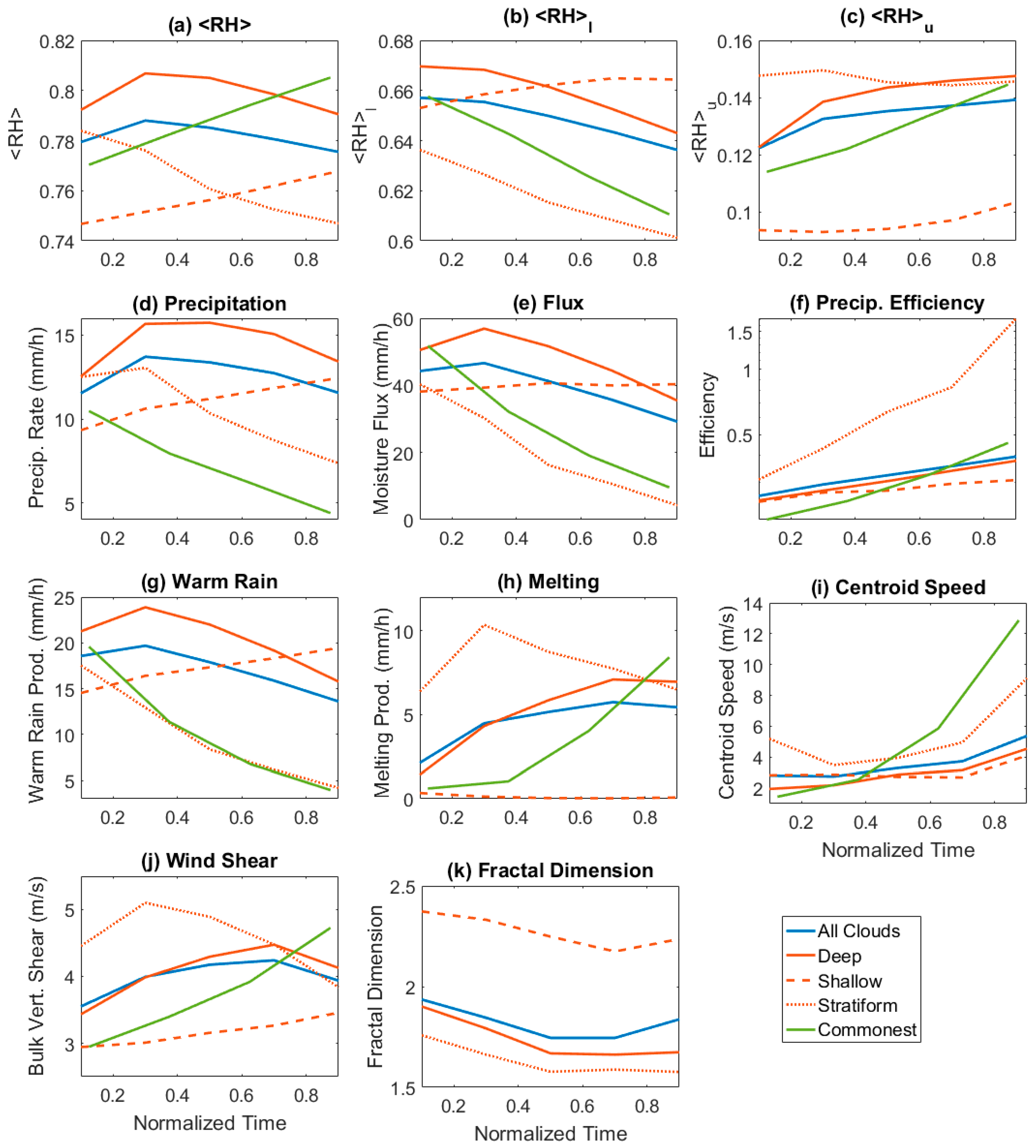
  • The P(<RH>) relationship is potentially a superposition of the relationships generated by upper and lower layer moisture (as in Igel [27]). Clouds tends to decrease <RH>l and increase <RH>u through convection over their lifetime, but not at the same rate, nor at a consistent one between clouds. This results in a non-monotonic evolution of <RH> and the slight deviation from 1-to-1 equation of P and <RH> over cloud lifetime seen in Masunaga [51].
  • Cloud PE increases with age. An object with increasing PE was offered as a working definition for the temporal evolution of a cloud. An increasing PE provides a definite termination to heavily precipitating clouds since it implies that eventually, precipitation will exhaust available moisture for its formation.
  • The surface shadow-projection fractal dimension is not constant throughout the lifetime of a cloud object. This could be important for entrainment, as it implies that the relationship between the horizontal cross-sectional area of an updraft and the updraft’s lateral exposure to dry air is not constant. Figure 3 suggests that entrainment should be higher during the initial phase (which is disproportionately highly made up of shallow convection), and that the final decay phase (which is similarly highly made up of stratiform cloud) should have higher entrainment per unit of horizontal area of cloud. This would slow initial growth of convection and hasten final decay, while providing relative enhancement to convection during the deep convective stage.
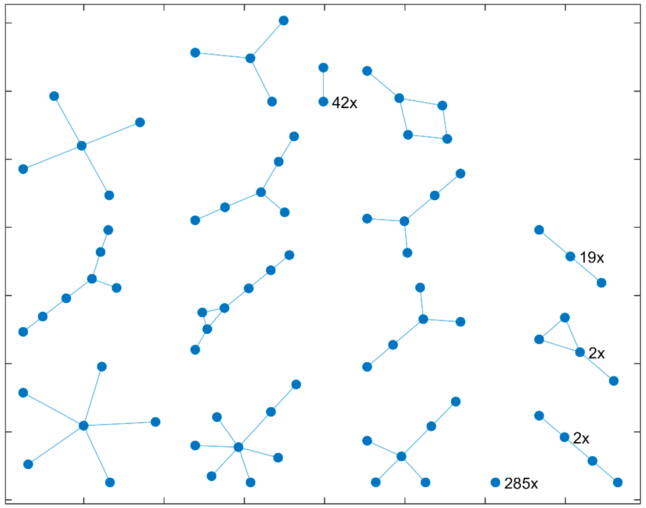
  • About half of the clouds identified result from a split or result in a merger at some point in their lifetime. Because many clouds that split or merge do so multiple times, clouds with complicated histories like these make up only a small fraction of the total population. 21% of clouds result from splits from another object. 16% of clouds merge with another. 2% of clouds see both a split and merger. 6% split and remerge. Splits and mergers do not seem to affect P(<RH>) significantly.
  • The speed at which a Lagrangian cloud object’s centroid moves is not constant through its lifetime. Relatively fast movement late in an object’s lifetime leads to ambiguity when comparing Eulerian or surface-based observations with Lagrangian ones that follow a cloud through 3D space.
  • Results suggest that the relationship between moisture and precipitation is a causal one. While it appears that moisture most often causes precipitation, the reverse relationship cannot be ruled out.
In addition to these conclusions, the results from this implementation of RAMStracks indicate that the actions and properties of convection are highly variable. Variability does not preclude drawing general conclusions and prototype evolutions (as above), but it does serve to emphasize that bulk measures of cloud environment (e.g., shear and <RH>) may be poor predictors of the behavior of individual clouds.

Funding

This material is based upon work supported by the National Science Foundation under Award No. 1433164.

Acknowledgments

The author would like to acknowledge high-performance computing support from Yellowstone (ark:/85065/d7wd3xhc) provided by NCAR’s Computational and Information Systems Laboratory, sponsored by the National Science Foundation. Updated versions of RAMStracks are available from the author’s website. The repository version is available at https://doi.org/10.7910/DVN/8VEUDC. The author would like to thank the reviewers who made many helpful suggestions.

Conflicts of Interest

The authors declare no conflict of interest.

References

  1. Houze, R.A. Mesoscale convective systems. Rev. Geophys. 2004, 42, 1–43. [Google Scholar] [CrossRef]
  2. Mapes, B.; Tulich, S.; Lin, J.; Zuidema, P. The mesoscale convection life cycle: Building block or prototype for large-scale tropical waves? Dyn. Atmos. Ocean. 2006, 42, 3–29. [Google Scholar] [CrossRef]
  3. Ruppert, J.H.; Johnson, R.H. Diurnally Modulated Cumulus Moistening in the Pre-Onset Stage of the Madden–Julian Oscillation during DYNAMO. J. Atmos. Sci. 2014, 72, 1622–1647. [Google Scholar] [CrossRef]
  4. Futyan, J.M.; Del Genio, A.D. Deep Convective System Evolution over Africa and the Tropical Atlantic. J. Clim. 2007, 20, 5041–5060. [Google Scholar] [CrossRef]
  5. Fiolleau, T.; Roca, R. Composite life cycle of tropical mesoscale convective systems from geostationary and low Earth orbit satellite observations: Method and sampling considerations. Q. J. R. Meteorol. Soc. 2013, 139, 941–953. [Google Scholar] [CrossRef]
  6. Hamada, A.; Takayabu, Y.N. Convective cloud top vertical velocity estimated from geostationary satellite rapid-scan measurements. Geophys. Res. Lett. 2016, 43, 5435–5441. [Google Scholar] [CrossRef]
  7. Feng, Z.; Dong, X.; Xi, B.; McFarlane, S.A.; Kennedy, A.; Lin, B.; Minnis, P. Life cycle of midlatitude deep convective systems in a Lagrangian framework. J. Geophys. Res. 2012, 117, D23201. [Google Scholar] [CrossRef]
  8. Chakraborty, S.; Fu, R.; Massie, S.T.; Stephens, G. Relative influence of meteorological conditions and aerosols on the lifetime of mesoscale convective systems. Proc. Natl. Acad. Sci. USA 2016, 113, 7426–7431. [Google Scholar] [CrossRef] [PubMed]
  9. Dixon, M.; Wiener, G. TITAN: Thunderstorm Identificaton, Tracking, Analysis and Nowcasting—A Radar-based Methodology. J. Atmos. Ocean. Technol. 1993, 10, 785–797. [Google Scholar] [CrossRef]
  10. Steinacker, R.; Dorninger, M.; Wolfelmaier, F.; Krennert, T. Automatic Tracking of Convective Cells and Cell Complexes from Lightning and Radar Data. Meteorol. Atmos. Phys. 2000, 72, 101–110. [Google Scholar] [CrossRef]
  11. Hagos, S.; Feng, Z.; McFarlane, S.; Leung, L.R. Environment and the Lifetime of Tropical Deep Convection in a Cloud-Permitting Regional Model Simulation. J. Atmos. Sci. 2013, 70, 2409–2425. [Google Scholar] [CrossRef]
  12. Caine, S.; Lane, T.P.; May, P.T.; Jakob, C.; Siems, S.T.; Manton, M.J.; Pinto, J. Statistical assessment of tropical convection-permitting model simulations using a cell-tracking algorithm. Mon. Weather Rev. 2012, 141, 557–581. [Google Scholar] [CrossRef]
  13. Dawe, J.T.; Austin, P.H. Statistical analysis of an LES shallow cumulus cloud ensemble using a cloud tracking algorithm. Atmos. Chem. Phys. 2012, 12, 1101–1119. [Google Scholar] [CrossRef] [Green Version]
  14. Heiblum, R.H.; Altaratz, O.; Koren, I.; Feingold, G.; Kostinski, A.B.; Khain, A.P.; Ovchinnikov, M.; Fredj, E.; Dagan, G.; Pinto, L.; et al. Characterization of cumulus cloud fields using trajectories in the center of gravity versus water mass phase space: 1. Cloud tracking and phase space description. J. Geophys. Res. Atmos. 2016, 121, 6336–6355. [Google Scholar] [CrossRef]
  15. Heiblum, R.H.; Altaratz, O.; Koren, I.; Feingold, G.; Kostinski, A.B.; Khain, A.P.; Ovchinnikov, M.; Fredj, E.; Dagan, G.; Pinto, L.; et al. Characterization of cumulus cloud fields using trajectories in the center of gravity versus water mass phase space: 2. Aerosol effects on warm convective clouds. J. Geophys. Res. Atmos. 2016, 121, 6356–6373. [Google Scholar] [CrossRef]
  16. Bretherton, C.S.; Peters, M.E.; Back, L.E. Relationships between Water Vapor Path and Precipitation over the Tropical Oceans. J. Clim. 2004, 17, 1517–1528. [Google Scholar] [CrossRef]
  17. Neelin, J.D.; Peters, O.; Hales, K. The Transition to Strong Convection. J. Atmos. Sci. 2009, 66, 2367–2384. [Google Scholar] [CrossRef]
  18. Peters, O.; Neelin, J.D. Critical phenomena in atmospheric precipitation. Nat. Phys. 2006, 2, 393–396. [Google Scholar] [CrossRef] [Green Version]
  19. Holloway, C.E.; Neelin, J.D. Moisture Vertical Structure, Column Water Vapor, and Tropical Deep Convection. J. Atmos. Sci. 2009, 66, 1665–1683. [Google Scholar] [CrossRef]
  20. Posselt, D.J.; van den Heever, S.; Stephens, G.; Igel, M.R. Changes in the Interaction between Tropical Convection, Radiation, and the Large-Scale Circulation in a Warming Environment. J. Clim. 2012, 25, 557–571. [Google Scholar] [CrossRef] [Green Version]
  21. Yano, J.-I.; Liu, C.; Moncrieff, M.W. Self-Organized Criticality and Homeostasis in Atmospheric Convective Organization. J. Atmos. Sci. 2012, 69, 3449–3462. [Google Scholar] [CrossRef]
  22. Ahmed, F.; Schumacher, C. Convective and stratiform components of the precipitation-moisture relationship. Geophys. Res. Lett. 2015, 42, 10453–10462. [Google Scholar] [CrossRef]
  23. Schiro, K.A.; Neelin, J.D.; Adams, D.K.; Lintner, B.R. Deep Convection and Column Water Vapor over Tropical Land vs. Tropical Ocean: A comparison between the Amazon and the Tropical Western Pacific. J. Atmos. Sci. 2016, 73, 4043–4063. [Google Scholar] [CrossRef]
  24. Igel, M.R.; Herbener, S.R.; Saleeby, S.M. The tropical precipitation pickup threshold and clouds in a radiative convective equilibrium model: 1. Column moisture. J. Geophys. Res. Atmos. 2017, 122, 6453–6468. [Google Scholar] [CrossRef]
  25. Holloway, C.E.; Neelin, J.D. Temporal relations of column water vapor and tropical precipitation. J. Atmos. Sci. 2010, 67, 1091–1105. [Google Scholar] [CrossRef]
  26. Kuo, Y.-H.; Neelin, J.D.; Mechoso, C.R. Tropical Convective Transition Statistics and Causality in the Water Vapor–Precipitation Relation. J. Atmos. Sci. 2017, 74, 915–931. [Google Scholar] [CrossRef]
  27. Igel, M.R. The tropical precipitation pickup threshold and clouds in a radiative convective equilibrium model: 2. Two-layer moisture. J. Geophys. Res. Atmos. 2017, 122, 6469–6487. [Google Scholar] [CrossRef]
  28. Plant, R.S. Statistical properties of cloud lifecycles in cloud-resolving models. Atmos. Chem. Phys. 2008, 9, 2195–2205. [Google Scholar] [CrossRef]
  29. Jirak, I.L.; Cotton, W.R.; McAnelly, R.L. Satellite and Radar Survey of Mesoscale Convective System Development. Mon. Weather Rev. 2003, 131, 2428–2449. [Google Scholar] [CrossRef] [Green Version]
  30. Cetrone, J.; Houze, R.A. Characteristics of Tropical Convection over the Ocean near Kwajalein. Mon. Weather Rev. 2006, 134, 834–853. [Google Scholar] [CrossRef]
  31. Simpson, J.; Keenan, T.D.; Ferrier, B.; Simpson, R.H.; Holland, G.J. Cumulus mergers in the maritime continent region. Meteorol. Atmos. Phys. 1993, 51, 73–99. [Google Scholar] [CrossRef]
  32. Cotton, W.R.; Pielke, R.A.; Walko, R.L.; Liston, G.E.; Tremback, C.J.; Jiang, H.; McAnelly, R.L.; Harrington, J.Y.; Nicholls, M.E.; Carrio, G.G.; et al. RAMS 2001: Current status and future directions. Meteorol. Atmos. Phys. 2003, 82, 5–29. [Google Scholar] [CrossRef]
  33. Meyers, M.P.; Walko, R.L.; Harrington, J.Y.; Cotton, W.R. New RAMS cloud microphysics parameterization. Part II: The two-moment scheme. Atmos. Res. 1997, 45, 3–39. [Google Scholar] [CrossRef] [Green Version]
  34. Saleeby, S.M.; Cotton, W.R. A large-droplet mode and prognostic number concentration of cloud droplets in the Colorado State University Regional Atmospheric Modeling System (RAMS). Part I: Module descriptions and supercell test simulations. J. Appl. Meteorol. 2004, 43, 182–195. [Google Scholar] [CrossRef]
  35. Saleeby, S.M.; Cotton, W.R. A binned approach to cloud-droplet riming implemented in a bulk microphysics model. J. Appl. Meteorol. Climatol. 2008, 47, 694–703. [Google Scholar] [CrossRef]
  36. Saleeby, S.M.; van den Heever, S.C. Developments in the CSU-RAMS aerosol model: Emissions, nucleation, regeneration, deposition, and radiation. J. Appl. Meteorol. Climatol. 2013, 52, 2601–2622. [Google Scholar] [CrossRef]
  37. Harrington, J.Y. The Effects of Radiative and Microphysical Processes on Simulation Warm and Transition Season Arctic Stratus. Ph.D. Thesis, Colorado State University, Fort Collins, CO, USA, June 1998. [Google Scholar]
  38. Romps, D.M.; Öktem, R. Stereo photogrammetry reveals substantial drag on cloud thermals. Geophys. Res. Lett. 2015, 42, 5051–5057. [Google Scholar] [CrossRef] [Green Version]
  39. Moseley, C.; Berg, P.; Haerter, J.O. Probing the precipitation life cycle by iterative rain cell tracking. J. Geophys. Res. Atmos. 2013, 118, 13361–13370. [Google Scholar] [CrossRef]
  40. Bretherton, C.S.; Blossey, P.N.; Khairoutdinov, M. An Energy-Balance Analysis of Deep Convective Self-Aggregation above Uniform SST. J. Atmos. Sci. 2005, 62, 4273–4292. [Google Scholar] [CrossRef] [Green Version]
  41. Muller, C.J.; Held, I.M. Detailed Investigation of the Self-Aggregation of Convection in Cloud-Resolving Simulations. J. Atmos. Sci. 2012, 69, 2551–2565. [Google Scholar] [CrossRef] [Green Version]
  42. May, P.T.; Ballinger, A. The statistical characterization of convective cells in a monsoon regime (Darwin, northern Australia). Mon. Weather Rev. 2007, 135, 82–92. [Google Scholar] [CrossRef]
  43. Igel, M.R.; Drager, A.J.; van den Heever, S.C. A CloudSat cloud object partitioning technique and assessment and integration of deep convective anvil sensitivities to sea surface temperature. J. Geophys. Res. Atmos. 2014, 119, 515–535. [Google Scholar] [CrossRef]
  44. Igel, M.R.; van den Heever, S.C. The relative importance of environmental characteristics on tropical deep convective morphology as observed by CloudSat. J. Geophys. Res. Atmos. 2015, 120, 4304–4322. [Google Scholar] [CrossRef]
  45. Witte, M.K.; Chuang, P.Y.; Feingold, G. On clocks and clouds. Atmos. Chem. Phys. 2014, 14, 6729–6738. [Google Scholar] [CrossRef] [Green Version]
  46. Bouniol, D.; Roca, R.; Fiolleau, T.; Poan, D.E. Macrophysical, microphysical and radiative properties of tropical Mesocale Convective Systems over their life cycle. J. Clim. 2016, 29, 3353–3371. [Google Scholar] [CrossRef]
  47. Hagos, S.; Feng, Z.; Landu, K.; Long, C.N. Advection,moistening, and shallow-to-deep convection transitions during the initiation and propagation of Madden-Julian Oscillation. J. Adv. Model 2014, 938–949. [Google Scholar] [CrossRef]
  48. Masunaga, H. A Satellite Study of the Atmospheric Forcing and Response to Moist Convection over Tropical and Subtropical Oceans. J. Atmos. Sci. 2012, 69, 150–167. [Google Scholar] [CrossRef]
  49. Duncan, D.I.; Kummerow, C.D.; Elsaesser, G.S. A Lagrangian Analysis of Deep Convective Systems and Their Local Environmental Effects. J. Clim. 2014, 27, 2072–2086. [Google Scholar] [CrossRef]
  50. Pauluis, O.; Schumacher, J. Radiation Impacts on Conditionally Unstable Moist Convection. J. Atmos. Sci. 2013, 70, 1187–1203. [Google Scholar] [CrossRef]
  51. Masunaga, H. Short-Term versus Climatological Relationship between Precipitation and Tropospheric Humidity. J. Clim. 2012, 25, 7983–7990. [Google Scholar] [CrossRef]
  52. Mapes, B.; Milliff, R.; Morzel, J. Composite Life Cycle of Maritime Tropical Mesoscale Convective Systems in Scatterometer and Microwave Satellite Observations. J. Atmos. Sci. 2009, 66, 199–208. [Google Scholar] [CrossRef]
  53. Sherwood, S.C.; Wahrlich, R. Observed Evolution of Tropical Deep Convective Events and Their Environment. Mon. Weather Rev. 1999, 127, 1777–1795. [Google Scholar] [CrossRef]
  54. Cahalan, R.F.; Joseph, J.H. Fractal Statistics of Cloud Fields. Mon. Weather Rev. 1989, 117, 261–272. [Google Scholar] [CrossRef] [Green Version]
  55. Lovejoy, S. Area-Perimeter Relation for Rain and Cloud Areas. Science 1982, 216, 185–187. [Google Scholar] [CrossRef] [PubMed]
  56. Batista-Tomás, A.R.; Díaz, O.; Batista-Leyva, A.J.; Altshuler, E. Classification and dynamics of tropical clouds by their fractal dimension. Q. J. R. Meteorol. Soc. 2016, 142, 983–988. [Google Scholar] [CrossRef]
  57. Bellenger, H.; Yoneyama, K.; Katsumata, M.; Nishizawa, T.; Yasunaga, K.; Shirooka, R. Observation of Moisture Tendencies Related to Shallow Convection. J. Atmos. Sci. 2015, 72, 641–659. [Google Scholar] [CrossRef] [Green Version]
  58. Taylor, G.I. Statistical theory of turbulence. Proc. R. Soc. London Ser. A 1935, 151, 421–444. [Google Scholar] [CrossRef]
  59. Kulp, C.W.; Zunino, L. Discriminating chaotic and stochastic dynamics through the permutation spectrum test. Chaos Interdiscip. J. Nonlinear Sci. 2014, 24, 033116. [Google Scholar] [CrossRef] [PubMed] [Green Version]
  60. Parlitz, U.; Berg, S.; Luther, S.; Schirdewan, A.; Kurths, J.; Wessel, N. Classifying cardiac biosignals using ordinal pattern statistics and symbolic dynamics. Comput. Biol. Med. 2012, 42, 319–327. [Google Scholar] [CrossRef] [PubMed]
  61. Glenn, I.B.; Krueger, S.K. Connections matter: Updraft merging in organized tropical deep convection. Geophys. Res. Lett. 2017, 44, 7087–7094. [Google Scholar] [CrossRef]
  62. Tao, W.-K.; Simpson, J. Cloud interactons and merging: numerical simulations. J. Atmos. Sci. 1984, 41, 2901–2917. [Google Scholar] [CrossRef]
  63. Lochbihler, K.; Lenderink, G.; Siebesma, A.P. The spatial extent of rainfall events and its relation to precipitation scaling. Geophys. Res. Lett. 2017, 44, 8629–8636. [Google Scholar] [CrossRef] [Green Version]
  64. Granger, C.W.J. Investigating Causal Relations by Econometric Models and Cross-spectral Methods. Econometrica 1969, 37, 424–438. [Google Scholar] [CrossRef]
Figure 1. The P(<RH>) relationship for all shadow points for all clouds over the tracking period (the final 3 days of the simulation) (‘Tracked Clouds’; red), the subset of those pixels occurring just before a split (gold), and just before a merger (purple), and the control P(<RH>) (‘All Points’) from the hourly output of the final 11 days of the simulation (blue).
Atmosphere 09 00289 g001
Figure 2. A snapshot of the horizontal distribution of <RH> in a small section of the simulation domain (colored contours; same color scheme as Igel et al. [24]). Regions of <RH>l over 0.63 (thick, blue contour) and <RH>u over 0.14 (thick, pink contour). Centroid locations of clouds tracked during hour 1428 (black, orange, yellow, and white).
Atmosphere 09 00289 g002
Figure 3. Mean normalized temporal evolutions of various cloud and environmental quantities for tracked clouds for all cloud (blue), various cloud types (reds), and for the clouds exhibiting the most common pattern (green; see Figure 4). The various panels indicate the normalized evolutions of (a) <RH>, (b) <RH>l, (c) <RH>u, (d) the precipitation rate, (e) the moisture flux, (f) the precipitation efficiency, (g) the warm rain generation, (h) the generation of rain due to melting, (i) the speed of the motion of the centroid location, (j) the magnitude of mean wind shear, and (k) the fractal dimension of the cloud.
Atmosphere 09 00289 g003
Figure 4. The fractional frequency among all tracked clouds that the normalized evolution for each cloud and environmental quantity exhibits the listed pattern number. Some example common pattern shapes. The various panels indicate the relative frequency of occurrence of the variable ordinal patterns for (a) <RH>, (b) <RH>l, (c) <RH>u, (d) the precipitation rate, (e) the moisture flux, (f) the precipitation efficiency, (g) the warm rain generation, (h) the generation of rain due to melting, (i) the speed of the motion of the centroid location, and (j) the magnitude of mean wind shear.
Atmosphere 09 00289 g004
Figure 5. Visual interpretation of the split and merger links between clouds. Dots represent individual clouds (i.e., CloudIDs) and lines represent splits or mergers of clouds. The labels indicate the number of times that the combination represented occurs in the data. As an example, the two dots, connected by a line, labeled ’42 ×’ indicates that there are 42 instances of a cloud originating from a split with another cloud or culminating in a merger.
Atmosphere 09 00289 g005
Figure 6. (Left side) scatter and regression of initial moisture((a) <RH>, (c) <RH>l, (e) <RH>U) onto the maximum intensity of precipitation. (Right side) the regression of maximum precipitation onto final moisture ((b) <RH>, (d) <RH>l, (f) <RH>U) (i.e., regression is performed on the inverse of the axes plotted).
Atmosphere 09 00289 g006
Table 1. Cloud and environmental quantities included in RAMStracks.
Quantity NameMeaningSize per CloudShell
CloudIDUnique numerical object identifier1-
CentroidX-Y location of shadow projection; Z of cloudt × 3-
ParentIDMarks Mergers0 to 1-
ChildIDMarks Splits0 to 4-
PCentroid Precipitation Rate (mm/h)tNo
<RH>lCentroid 0–4 km contribution to <RH> ([27])tNo
<RH>uCentroid 4–14 km contribution to <RH> ([27])tNo
All_PPrecip. Rate for all shadow columns (mm/h)t × nYes
All_<RH>l<RH>l for all shadow columnst × nYes
All_<RH>u<RH>u for all shadow columnst × nYes
FinalTimeLast time step object is identified1-
MaALShadow major axis lengthtNo
MiALShadow minor axis lengthtNo
OrientationMaAL directiontNo
AreaNumber of 3D pixelstYes
PerimeterNumber of shadow edge pixelstNo
FluxVertical moisture flux 1–14 km (mm/h)t × nYes
ShearBulk vertical wind shear (m/s)t × nYes
WRWarm rain production (mm/h) ([24])t × nYes
MtMelting to rain (mm/h) ([24])t × nYes
TypeEstimated primary cloud type1No
SpeedCentroid velocity (m/s)t × (n − 1)No
ShellIDNumerical shell identifiertOnly
RegimeIgel [27] “ regime“ fraction of shadow pixelst × 4No
Table 2. The fraction of clouds for which one quantity granger causes the corresponding quantity.
Causes PrecipitationPrecipitation Cause
Lifetime1st Half2nd HalfLifetime1st Half2nd Half
<RH>68%80%71%57%71%63%
<RH>l69%83%72%56%75%60%
<RH>u57%74%63%51%69%61%

