1. Introduction
The atmospheric boundary layer (ABL) is the lowest part of the atmosphere where the Earth’s surface strongly influences the wind, temperature, and humidity through turbulent transport of air mass. Due to its superior importance for the atmosphere system, an appropriate representation of the ABL is essential for both operational numerical weather prediction (NWP) and climate models as well as for a wide range of practical applications, such as air pollution forecast and wind energy yield estimates. In contrast to the ABL, the stable boundary layer (SBL) is typically one order of magnitude shallower and can reach a vertical extent as low as 10
. Turbulence in the SBL is typically much weaker or intermittent and is mainly produced by vertical wind shear, whereas buoyancy inhibits vertical motion. Furthermore, a number of nonturbulent motions, such as wave-like motions, solitary modes, microfronts or drainage flows, become important [
1]. The principal problem in representing turbulence in those models correctly is that the length scales of the turbulent processes are typically far below model resolution and therefore need to be parameterized. While the corresponding parameterization schemes, e.g., reference [
2], generally work very well for near-neutral and unstable conditions, they show significant shortcomings for the SBL, e.g., by systematically overestimating turbulent mixing rates and the height of the ABL (
) [
3,
4,
5,
6]. In the context of weather forecasting, this leads to, amongst others, significant errors in the prediction of near surface parameters, such as the 2-m temperature and 10-m wind speed for situations with clear skies and low wind typically occurring at night or during winter [
6]. Errors in
might also induce considerable uncertainties in the forecast of wind profiles and the location of low-level jets (LLJ), which are crucial parameters for applications such as wind energy. Furthermore, this also leads to a typical warm bias for SBL conditions in NWP models [
4,
7,
8], which is also of importance under the aspects of climate and climate change. One of the most dominant signals in climate records is the accelerated warming of the polar regions during wintertime and the increase in nighttime temperatures at lower latitudes [
9]. This observed polar amplification may be partly related to the shallow SBL with a corresponding small heat capacity. Hence, a certain heat gain results in a relatively large temperature increase [
10]. In addition, this dampens the temperature inversion infrared cooling to space [
11,
12]. A systematic overestimation of turbulent mixing and the ABL height thus complicates the proper attribution of the mechanisms of Arctic climate change [
12,
13,
14].
Monin–Obukhov similarity theory (MOST) provides dimensionless relationships between the surface fluxes of heat and momentum, the variance and the mean gradients of temperature, moisture, and wind in the atmospheric surface layer (SL). These dimensionless relationships are a function of the height (
z) above the surface, which is made dimensionless with the Monin–Obukhov length scale (
L). Strictly speaking, these relationships apply only for stationary and homogeneous surface conditions. In practice, however, there is a strong need for wider application, and as such, field observations in a variety of circumstances are needed to evaluate the dimensionless relationships. Most of the surface parameterization schemes in NWP and climate models are based on the traditional MOST, which is known for its shortcomings in characterizing the SBL [
15,
16,
17,
18,
19,
20,
21]. Under such conditions, continuous turbulence may break down and become intermittent e.g., [
22], so that non-local features, such as the stability at higher levels and the Coriolis effect, gain relative importance [
23,
24]. This may imply the occurrence of upside-down events, in which turbulence is mainly generated by the vertical wind shear associated with LLJ [
23,
25]. Additional processes, such as inertial oscillations and gravity waves [
26] can then contribute significantly to the turbulent kinetic energy (TKE) budget. Zilitinkevich and Calanca [
15] and Zilitinkevich [
27] presented an attempt for a non-local theory for the SBL, taking into account the effect of internal gravity waves in the free atmosphere. In addition, other small-scale processes and phenomena, such as drainage flow, radiation divergence [
1,
6,
28], fog, and close interactions with the surface as well as potential snow feedback [
29] further increase the complexity of the SBL. The effects of all those phenomena are neither well understood, nor sufficiently captured by MOST or its extensions [
15,
30,
31,
32].
SBL conditions also impose challenges with respect to observations, as the typically weak turbulent fluxes close to the surface become difficult to measure precisely under very stable conditions. Gradient-based scaling schemes, as proposed by [
20,
33,
34] and formally equivalent to the MOST approach, might overcome some of the observational issues of weak turbulent fluxes, since the vertical gradients within the SBL are usually strong and relatively easy to measure. From a modeling point of view, recent high-resolution large-eddy simulation (LES) studies have shown a lack of grid convergence under stable conditions [
35,
36,
37] which might be attributed to the fact that MOST is usually applied between the surface and the first grid level in the atmosphere (i.e., typically at heights between 1
to 10
). This might violate basic assumptions for MOST, e.g., that the measurement level or the first grid level in LES cases must lie inside the inertial sublayer, in which the flow is spatially homogeneous and dissipation follows Kolmogorov’s 5/3 law. Errors can be induced by the fact that turbulence is not properly resolved at the first couple of grid points adjacent to the surface. In such cases, turbulence is not fully resolved and the flow is dominated by the subgrid-scale model in use. It is often observed that this general deficiency of LES models to resolve turbulence near the surface leads to near-surface gradients that are too strong and inherently lead to an underestimation of the surface friction [
38].
Field campaigns addressing the SBL generally face logistical challenges in taking measurements at remote sites that are difficult to reach and are often characterized by harsh weather conditions, especially in regard to low temperatures. In particular, observations over sea ice involve additional risks for equipment and people, e.g., due to sea ice motion and melt. Major campaigns with focus on the SBL over sea ice have included the Weddell ice station in the Austral autumn and winter of 1992 [
39,
40,
41,
42], the Surface Heat Budget over the Arctic Ocean (SHEBA) in the Beaufort Sea in 1997–1998 [
23,
43,
44], the drifting ice station, Tara, in the central Arctic in the spring and summer of 2007 [
45,
46,
47], and the drifting station, N-ICE2015, north of Svalbard in the winter and spring of 2015 [
48]. Other land-based campaigns, e.g., ARTIST [
49], CASES-99 [
50], GABLS [
51,
52], FLOSS-II [
53], the measurements at Summit Station in central Greenland [
54], and recently, MATERHORN [
55] have also contributed considerably to the current state of knowledge on SBLs. The typical observation methods applied in such campaigns are profile measurements using weather masts, tethersondes, and radiosondes, as well as eddy covariance (EC) measurements at one or multiple levels. Several SBL studies have also been based on manned research aircraft observations, mainly over sea ice in the Arctic [
56,
57,
58,
59,
60] and the Baltic Sea [
61,
62]. Manned research aircraft may also release dropsondes and apply airborne LIDARs [
63]. Over the last decade, the use of Unmanned Aerial Vehicles (UAVs) has also rapidly increased in the field of atmospheric research [
64,
65] and corresponding systems have been applied in ABL campaigns, both in the Arctic [
66,
67,
68] and Antarctic [
69,
70,
71,
72,
73].
The different methods for observing the SBL are generally complementary. Continuous time series of basic meteorological parameters at different temporal resolutions can be obtained in-situ by weather masts, tethersondes, or radiosonde ascents, or they can be remotely sensed by e.g., with LIDAR (Light Detection and Ranging), SODAR (Sound Detection and Ranging), RADAR (Radio Detection and Ranging), RASS (Radar-Acoustic Sounding System) or microwave radiometer observations. All these measurement methods and devices have certain shortcomings that may be at least partially overcome by proper UAV missions. Weather masts are limited in height and are rather inflexible with respect to changes in location. Tethersondes require considerable infrastructure and their operation is limited to wind speeds below 12
−1 [
47]. Continuous data are only available if the balloon is kept at a fixed altitude, which limits the vertical resolution [
74]. In addition, sometimes the temperature inversions can be so strong that the buoyancy of the tethered balloon is not sufficient to penetrate it [
67]. Rawinsonde soundings reach high altitudes, but pass very quickly through the interesting layers for SBL research. They only provide snapshots of vertical profiles in relatively poor temporal resolution, and are comparatively expensive for long-term use. Observations by large manned research aircraft are even more expensive. An additional drawback of those platforms for SBL research is the limitation in the lowermost possible flight altitude for safe operations and the fact that the pure size and velocity of the aircraft might massively disturb the local structure and dynamics of a shallow SBL. Doppler LIDARs and SODARs provide wind information with a vertical resolution in the order of 5
to 20
, typically in the lowest few hundred meters above the ground, depending on wind speed and stability, and, in the case of LIDAR, also on other parameters, such as the aerosol content [
75], water vapor, ozone or temperature. So far, the use of remote-sensing systems for dedicated SBL campaigns in polar regions has been rather limited, [
49,
76,
77]. Furthermore, the minimum altitude for wind information from pulsed non-scanning LIDAR systems is in the order of 40
. Higher vertical resolution and lower minimum altitudes can be achieved by operating scanning Doppler LIDARs at low-elevation angles. However, the achieved data originates from a much larger area than for high elevation scans. Scintillometers are capable of measuring spatially-averaged turbulent fluxes and cross-winds close to the ground along horizontal paths of approximately 1
to 10
. In previous years, SBLs have also been addressed by satellite-based remote-sensing, e.g., [
78].
The main motivation for the ISOBAR project is to develop and apply a new and innovative observation strategy for the SBL that is based on meteorological UAVs, ground-based in-situ, and remote-sensing profiling systems. The main idea is to combine the reliability and continuity of well-established ground-based observations with the flexibility of small UAV systems. This strategy is to be applied during several campaigns in polar regions to provide extensive data sets on the turbulent structure of the SBL with unique and unprecedented spatial and temporal resolution. This will form the basis for intensive analysis of small-scale turbulent processes in the SBL and corresponding multi-scale modeling studies.
To optimize the collection of ABL data over a period of three weeks, the Hailuoto-I campaign was based on the combined use of a weather mast, equipped for gradient and flux observations; a scanning Doppler LIDAR; a vertically pointing SODAR; and several fixed-wing and multicopter UAVs equipped with different sensors. To the authors’ knowledge, the Hailuoto-I campaign is the first field campaign to combine ground-based in-situ and remote-sensing instrumentation with the intensive use of multiple UAVs for systematic SBL research.
The manuscript is structured in the following way. In
Section 2 we describe the experiment site, the instrumentation used, and some details on the operation of our UAVs. Data processing methods and data availability are summarized in
Section 3.
Section 4 describes the general synoptic situation and the sea ice conditions during Hailuoto-I. The first results are presented in
Section 5 together with a brief discussion, before summarizing the main outcomes of the Hailuoto-I campaign and giving a short outlook on our future plans for specific analysis and modeling studies in
Section 6.
2. Experiment Description
The Hailuoto-I campaign took place between 11 and 27 February 2017 over the sea ice of the Bothnian Bay, close to the Finnish island of Hailuoto, as part of the ISOBAR project. Hailuoto island is located roughly 20
west of the city of Oulu and has a size of about 200
2 (
Figure 1). Its landscape is mainly flat heath terrain, with the highest point reaching only about 20
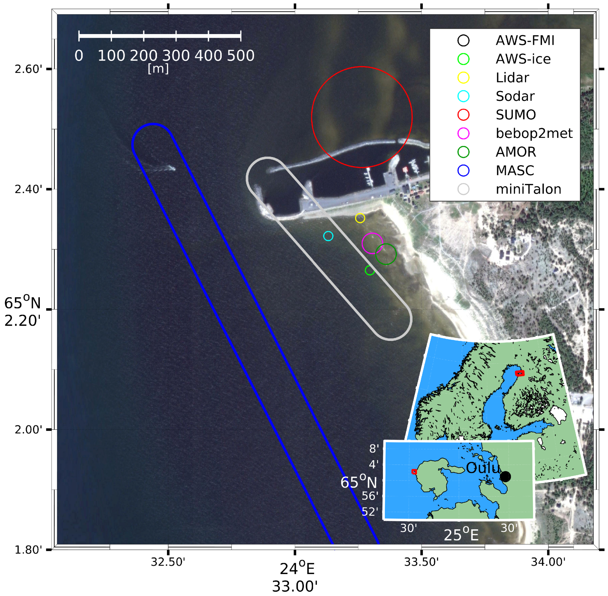
asl. The field site was located at 65.0384
N and 24.5549
E, just off-shore of Hailuoto Marjaniemi, the westernmost point of the island (
Figure 1), where the Finnish Meteorological Institute operates a permanent weather station. Bothnian Bay, the northernmost part of the Baltic Sea, is typically entirely frozen every winter with the exception of the winters of 2014/2015 [
79] and 2015/2016 with land-fast ice up to
on the coast of Hailuoto.
During the observation period, the apparent sunrise changed from 6:35 to 5:39 UTC and the apparent sunset from 14:38 to 15:31 UTC, calculated with [
80]. The noontime solar elevation angle ranged from 11.15
to 16.83
[
81]. The apparent solar and sea ice conditions favored the formation of a SBL [
61,
62], underlying a weak diurnal cycle.
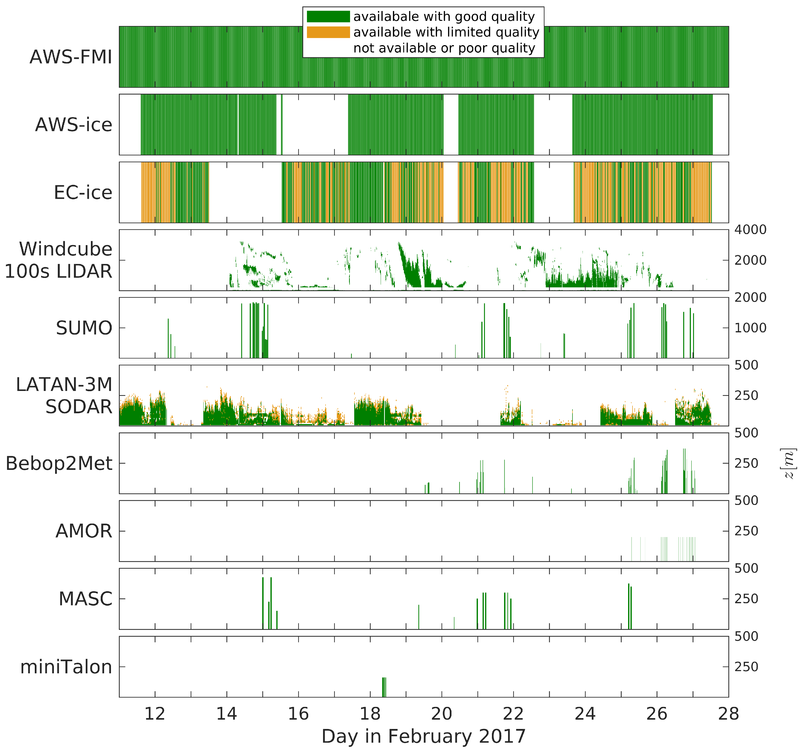
The instrumentation operated on site during the campaign included an eddy covariance (EC) system; a 4 m meteorological mast with three levels of slow-response sensors for temperature, humidity, and wind; a four component radiometer; and two ground flux sensors. The ground-based in-situ measurements were complemented by a scanning wind LIDAR, a vertically profiling SODAR, and several types of fixed and rotary-wing UAVs.
2.1. Instrumentation
2.1.1. Basic Instrumentation
Close to the selected field site, the Finnish Meteorological Institute (FMI) operates the World Meteorological Organization (WMO) automatic weather station (AWS) Hailuoto Marjaniemi (ID 02873), henceforth referred to as AWS-FMI. The Western and Northern sectors of this station represent open water conditions during summer and typically, sea ice during winter, which was also the case during this campaign, as will be later seen in
Section 4. East of the station (about 45
to 165
), the measurements are affected by the island and by some buildings at a distance of about 50
to 100
from the station, including a lighthouse and an ice radar tower. The measured parameters, installed instrumentation, and their heights are listed in
Table 1. All measurements, except wind, are collected at the station; the wind speed and direction are observed at the top of the ice radar tower. The anemometer is supported by a 2 m high mast attached to the railing of the tower platform, the measurement height being about 29
asl.
The Finnish Transport Agency operates a network of coastal ice radars used for ice monitoring for navigation along the Finnish coast. One of the radars is located at Marjaniemi, at the top of a 30-m high tower next to the AWS-FMI and the light house. The ice radar is a
(
), 25
magnetron radar manufactured by Terma A/S, Denmark. The range resolution (the pulse length) can be chosen operationally by Vessel Traffic Services depending on ice conditions and can vary from 50
to 1000
(pulse repetition frequency from about 0.7
to 3.5
). Rasterized images are provided with a temporal median filtering of 15
to 20
. However, due to the limited means of mobile data communication, preprocessed images can only be transmitted at 2-min intervals. More detailed information on the radar and image processing is provided in reference [
82].
A 4 m mast, from here on referred to as AWS-ice, equipped with instrumentation for observations of wind speed, direction, temperature and relative humidity (all at 1magl, 2magl and 4
agl, radiation balance, and ground heat flux (snow and ice), was installed on the sea ice (
Figure 1). For observations of SL turbulence, the mast was additionally equipped with an EC system, consisting of a 3-dimensional sonic anemometer and an open-path gas-analyzer for H
O and CO
, both mounted at
agl. The EC system faced towards 238
(true direction) in order to have an undisturbed fetch over the sea ice sector. The sensor specifications are summarized in
Table 2.
2.1.2. UAV Platforms
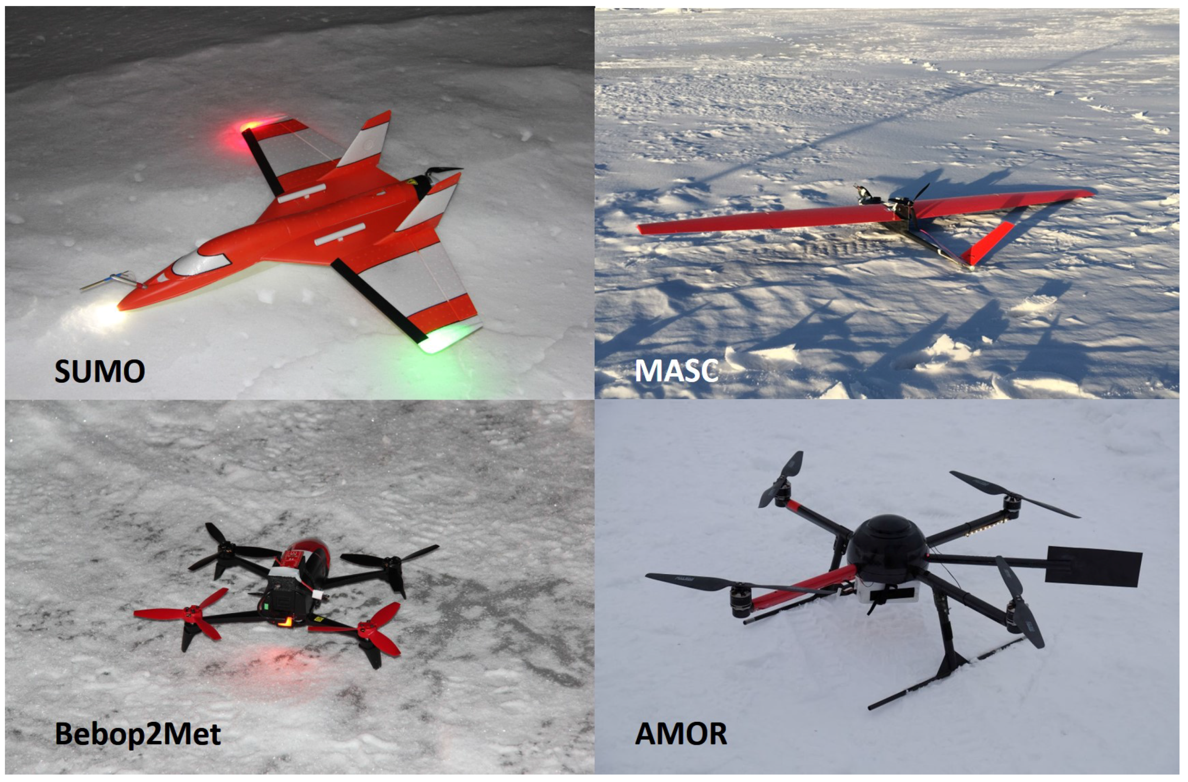
In order to obtain detailed information on the atmospheric state across the entire ABL and parts of the free atmosphere, a number of different UAV (
Figure 2), both fixed and rotary-wing systems, were operated in the area around the main field site. A short description of the systems used during the campaign and their capabilities are given below.
The Small Unmanned Meteorological Observer (SUMO) [
83,
84] is a small fixed-wing UAV, equipped with the Paparazzi autopilot system and a set of basic meteorological sensors. The data acquisition system of the SUMO also records the aircraft’s position and attitude, provided by an on-board Global Navigation Satellite System (GNSS) and an Inertial Measurement Unit (IMU). The SUMO is designed to take atmospheric profiles up to 5000
and can be operated in wind speeds of more than 15
−1. Under cold environmental conditions, the flight time is typically 45
. The most important sensor specifications are summarized in
Table 3. The meteorological sensors for
T and
are placed a fair distance from the battery and motor on top of the wings to assure good ventilation during flight. In addition to the directly-measured meteorological parameters, like temperature, relative humidity, and pressure, the horizontal wind speed and direction can be estimated by applying the “no-flow-sensor” wind estimation algorithm described in reference [
68].
The Multi-purpose Airborne Sensor Carrier (MASC-2) is an electrically-powered, single engine, pusher aircraft of
wing span and a total weight of 6
, including a scientific payload of
[
85]. This UAV is equipped with the ROCS (Research Onboard Computer System) autopilot system developed at the University of Stuttgart. Its endurance under polar conditions is up to 90
at a cruise speed of 22
−1. For the measurement of turbulence along horizontal straight flight legs and other atmospheric parameters, MASC-2 carries a scientific payload, as summarized in
Table 4 and described in detail in [
86,
87,
88]. The sensors are placed in a special sensor holding unit which is attached to the aircraft directly above the nose to face air that is as undisturbed as possible. The 3D-wind vector and the temperature measurements are capable of resolving turbulence up to frequencies of approximately 30
, allowing turbulent fluctuations to be resolved in the sub-meter range. The data from these sensors is oversampled with an acquisition frequency of 100
. Each component of the measurement system aboard MASC-2 was tested in the lab and during flight. The sensors were calibrated and airborne gathered data were validated by comparison to both other measurement systems and theoretical expectations [
85,
86,
87].
A new UAV based on the the miniTalon produced by X-UAV with an EPP airframe of 120
wingspan and 83
length that was designed to carry a higher payload (up to 1000
) was tested during the campaign. The system is a further development of the SUMO by Lindenberg und Müller GmbH & Co. KG and GFI, with increased dimensions. It allows for the integration of an additional turbulence sensor package (Aerosonde five-hole probe), significantly higher air speeds (up to 25
−1), and longer endurance (ca. 90
). The turbulence sensors are placed in the nose facing forward, whereas the temperature and humidity sensors are mounted on top of the fuselage, well separated from the battery and motor. Aside from these differences, the miniTalon is equipped with the same Paparazzi autopilot system and the same basic sensor package as described above (
Table 3).
The Bebop2Met is based on Bebop2 by Parrot, a small, commercially-available multicopter with a weight of about 500
and a diameter of roughly 50
. The system was modified for our purposes by adding meteorological sensors (
Table 3) integrated into a 3D-printed frame attached on top of the battery, as well as by running the Paparazzi autopilot software on the original processor. The sensors for
T and
are placed a few centimeters above one of the propellers on a thin side arm. Tests have shown that the sensors are well ventilated and that the flow at this location is fairly horizontal. The flight time under cold environmental conditions is typically in the range of 20
, and it can only be operated safely in weak and moderate wind conditions below 10
−1. Typical flight operations include maneuvers such as hovering at a fixed position and altitude and vertical profiles at a fixed location with a constant vertical speed.
The Advanced Mission and Operation Research (AMOR) multicopter UAV was designed to fly in environmental monitoring missions [
89], including meteorological campaigns in polar regions. The central airframe, the side arms, the landing gear, and the 15 inch propellers are made of carbon-reinforced plastic. The empty weight of the UAV is
, and the maximum takeoff weight is
. Depending on the environmental conditions, the battery, and the payload, the maximum flight time is approximately 60
, and the UAV can be operated in winds of up to 15
−1. Due to the cold conditions and the relatively short profiling missions during Hailuoto-I, AMOR flights took typically about 5
. The Advanced Meteorological Onboard Computer (AMOC) receives the sensor data, fuses the data sets with the IMU and GNSS data sets, and stores them on a µSD card. A fast temperature sensor based on a 25
thermocouple wire, a factory calibrated HYT 271 RH sensor, and a Digi Pico P14 Rapid RH sensor provide the meteorological standard data sets. A pressure sensor provides the altitude above ground level, and a Melexis thermopile sensor provides the surface temperature data, as shown in
Table 5. The sensors are mounted on a horizontal tube well outside the downwash of the propellers.
2.1.3. Remote-Sensing
For observations of the 3D-wind field over our study area, we deployed a scanning wind LIDAR (Leosphere Windcube 100s) on the shoreline (
Figure 1). The Windcube 100s is a pulsed wind LIDAR system operating at a wavelength of
and a pulse energy of about 10
. It has a maximum range for wind measurements of
at a range gate resolution of 50
. The LIDAR was operated in PPI (plan position indicator) mode, i.e., performing azimuth scans over 360
alternating between two elevation angles of 1° and 75
. Further details on the chosen settings are summarized in
Table 6.
A vertically-pointing, single-antenna version of the LATAN-3M SODAR system [
90] was installed on the sea ice at a distance of about 50
from the coastline (
Figure 1) on 8 February. The SODAR has a frequency-coded sounding signal which allows several measurements per range gate, thus providing higher data availability and quality compared to single-frequency signals. The frequency-coded signal includes eight consecutive 50
pulses with frequencies of 3.32, 3.46, 3.58, 3.66, 3.76, 3.9, 4.02 and 4.13
. The vertical measurement range is from 10
to 340
, even though the lowest and highest levels typically suffer from poor data availability. At the lowest 3 to 4 levels, the data availability is reduced, since measurements are only based on the first few frequencies as the sampling starts immediately after the transmission of the last frequency. On the other hand, the data availability from the upper levels is often limited by atmospheric conditions because of the lack of thermal turbulence from which the acoustic echoes originate. The measured parameters are the intensity within the main spectral peak of the return signal and the adjacent band and the Doppler shift of the peak, expressed in terms of radial velocity. The parameters are estimated for each range gate with 3
-resolution (
Hz). From the data, it is possible to derive, for example, profiles of mean vertical velocity and its variance. Previously, this SODAR has been used to detect wind shear driven turbulence, convective turbulence, strong katabatic flows, and moist air advection with wave structures in the stably stratified ABL [
91].
2.2. UAV Operations
Flights taking place at altitudes of less than 150
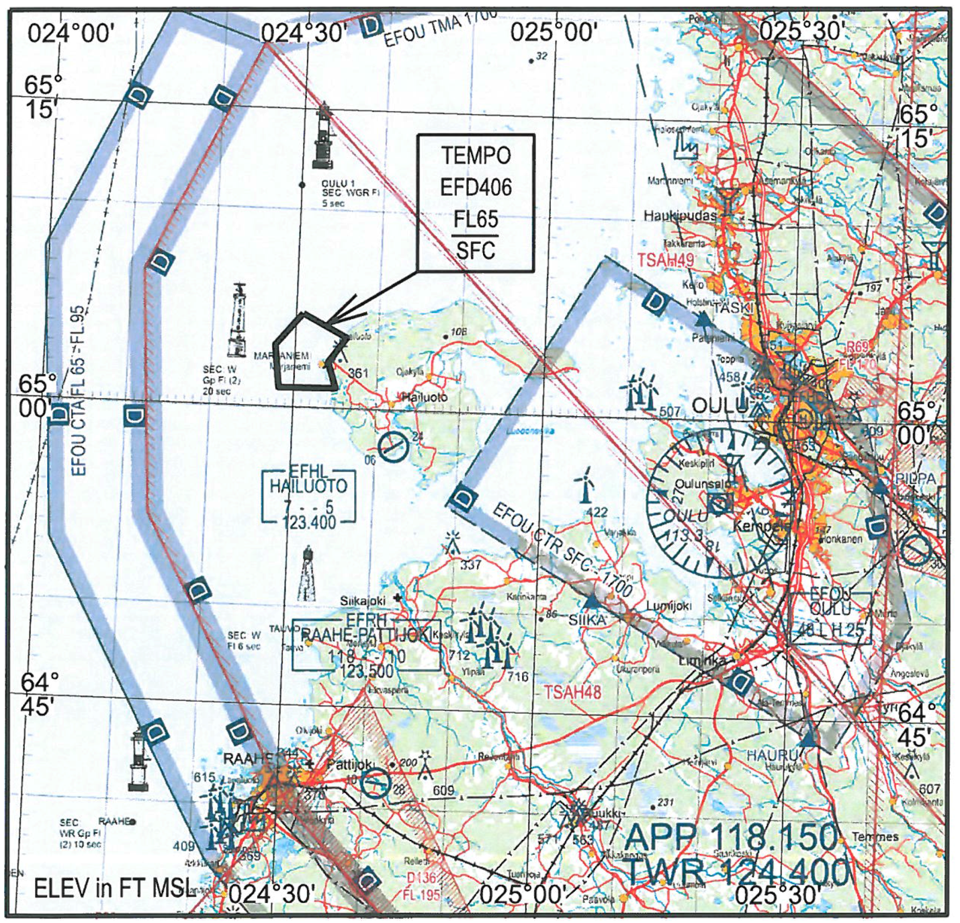
agl and with visual contact to the aircraft can be carried out without any restrictions. Since parts of our operations exceeded these limitations, specifically, the maximum allowed altitude, an application was made for the establishment of a temporary danger area (D-Area), which was granted by the Finnish Aviation Agency for the core period of our campaign. The D-Area (
Figure 3) extended from our field site 3
to 4
along the coast in Southern and Northeastern directions and about 5
off-coast to the west and northwest. The vertical extent was from the surface up to flight level 65 ( 6500 ft or
), but we limited our operations to a maximum target altitude of 1800
to ensure a good safety margin. The D-Area had to be reserved on a daily basis on the last working day preceding the activities by sending a corresponding request to the airspace management and control (AMC) unit. Before the actual start of UAV operations, we had to contact the responsible AMC unit at Oulu airport to activate the D-Area. If aircraft were passing through or other operations compromised flight safety, the AMC unit could contact us and all operations had to be cancelled immediately. The end of the UAV activities was again reported from our side to AMC to deactivate the D-Area.
The different aircraft types were used for specific missions in the vicinity of our ground-based measurement systems. The typical locations of these flight missions are indicated in
Figure 1. All UAVs applied could be operated with a few minutes delay between landing and the next launch, since this usually only requires the installation of new batteries and the start of a new flight mission in the GCS. Apart from MASC-2, which was started with the help of a bungee, all other UAVs could be launched without any technical support, i.e., from ground or hand launch for the multicopters and fixed-wing aircraft, respectively. However, only the multicopter systems, which were mainly used for ABL profiles, were operated at high repetition frequencies during intense observation periods.
The SUMO system can climb very efficiently and was mainly used to obtain vertical profiles up to an altitude of roughly 1800 . These profiles were achieved by a helical flight pattern with a radius of 120 and an ascent and descent rate of roughly 2 −1. The main purpose of these missions was to obtain several atmospheric profiles per day, covering the ABL and the lower part of the free atmosphere, reflecting larger scale variations in the atmospheric background state. In total, SUMO performed 39 scientific flights during the campaign.
The flight patterns of the MASC-2 and the miniTalon, which were both designed for airborne turbulence measurements, consisted of horizontal race tracks at different altitudes between 20 agl to 400 agl. The race tracks, two parallel straight legs of about 600 to 1500 length connected by half circles for turning the aircraft, were typically aligned in the main wind direction. The data observed with the high-resolution wind and temperature sensors on these legs were used to provide turbulent parameters at higher levels. MASC-2 flights were typically carried out several times per day and partially repeated after 2 . During the campaign, the miniTalon was only used for one day (three measurement flights) for testing and validation against the MASC-2 system, which was operated simultaneously. The data from these three miniTalon flights are not the subject of this article, since sophisticated data processing algorithms must be developed for the further analysis. The analysis of the 14 scientific MASC-2 flights is also beyond the scope of this article.
Two multicopter systems were utilized to obtain profiles at a very high vertical resolution within the ABL. In order to gain detailed information on the evolution of the ABL, these profiles were repeated almost continuously during intensive operation periods. Due to the more sophisticated sensor package with partially very short response times, the AMOR system is capable of probing the ABL with higher accuracy, whereas the Bebop2Met profiles are comparably smooth. However, this was partially compensated by operating the Bebop2Met at a slower ascent rate. Due to technical problems, the AMOR system could only be operated during the very end of our campaign.
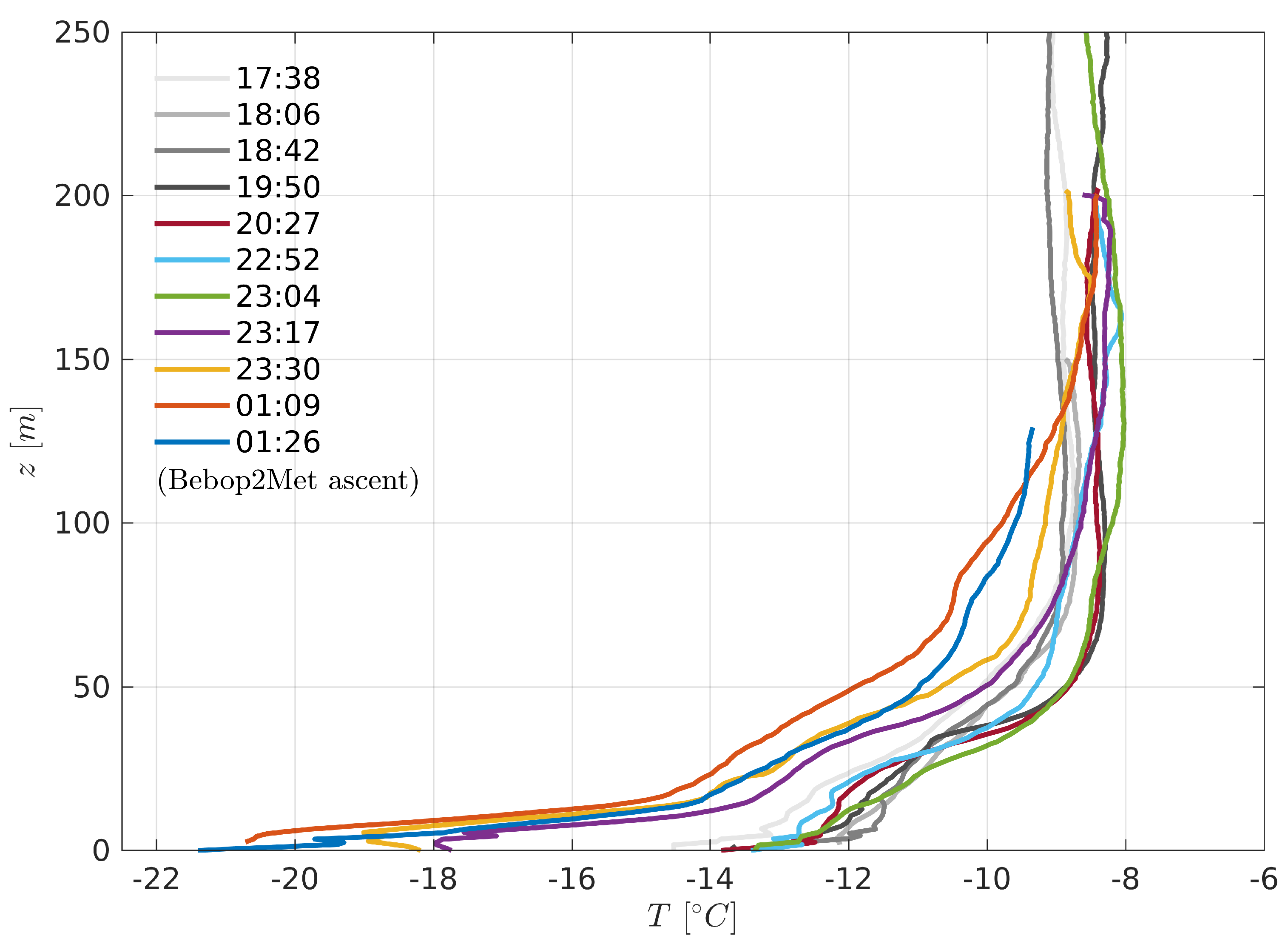
The Bebop2Met UAV was operated on vertical profiles, ranging from 0 agl and typically 200 agl or even higher ( 400 agl) when the atmospheric conditions allowed for it. The atmospheric profiles were performed at a fixed location at a distance of about 10 to 20 from the meteorological mast. In order to optimize the vertical resolution of these surface and boundary layer profiles, the vertical climb rate was set to −1 below 10 agl and 1 −1 above. The flights took typically 15 to 20 and could be repeated after a ground time of approximately 5 . For comparison to the mast observations and the calibration of the (experimental) wind estimation algorithm, the Bebop2Met was held at a fixed altitude of 2 agl to 4 agl for 1 to 2 .
The maximum height of the AMOR multicopter profiles was typically 200 agl. In order to operate the AMOR UAV safely in the vicinity of the other UAV and the meteorological mast on the sea ice, the start and landing site was chosen to be closer to the shore side. After the takeoff to 5 agl, the flight was continued at the final location of the profile, approximately 20 further towards the seaside. The lowest part of the ABL was sampled with a vertical climb speed of 1 −1, resulting in a very high temperature resolution of approximately .
4. Synoptic Situation and Sea Ice Conditions
The analysis of the synoptic situation, including the passages of fronts and sea ice conditions was based on the daily FMI operational weather analysis and ice charts. Until recently, the Bothnian Bay has been entirely frozen every winter. However, the ice thickness, the maximum annual ice extent, and the length of the ice season have shown decreasing trends in recent decades [
95]. Winters 2014/2015 (Uotila2015) and 2015/2016 were the first for which we can be certain that parts of the Bothnian Bay remained ice-free. The maximum ice extent is typically reached in March. In the shallow waters close to the coast, land-fast ice prevails and can grow up to a thickness of
. Even in mild winters, the level ice thickness reaches 0.3
to 0.5
. The land-fast ice is typically free of leads, and the compact sea ice field with snow pack on top effectively insulates the atmosphere from the relatively warm sea.
The sea ice season 2016/2017 was mild in the Baltic Sea. Its length in the Bothnian Bay was, however, close to the average of 1965–1986 (reference period used in FMI ice service). The ice growth started during the first half of November 2016 and was fast during a cold period in early January, leading to an overall ice extent of 44,000 km in Bothnian Bay. Shortly thereafter, temperatures increased and for the rest of the month, mild southwesterlies prevailed, preventing new ice formation and packing the ice densely towards the coast within Bothnian Bay. By the end of January, the Baltic Sea ice extent had reduced to only 28,000 km.
In the beginning of February, a large high pressure system strengthened over Finland, causing fair weather and occasional extremely cold temperatures. Especially from 6 to 9 February, there were very cold temperatures in most of the country. The ice extent increased then rapidly, and a maximum ice extent in the Baltic Sea of 88,000 km
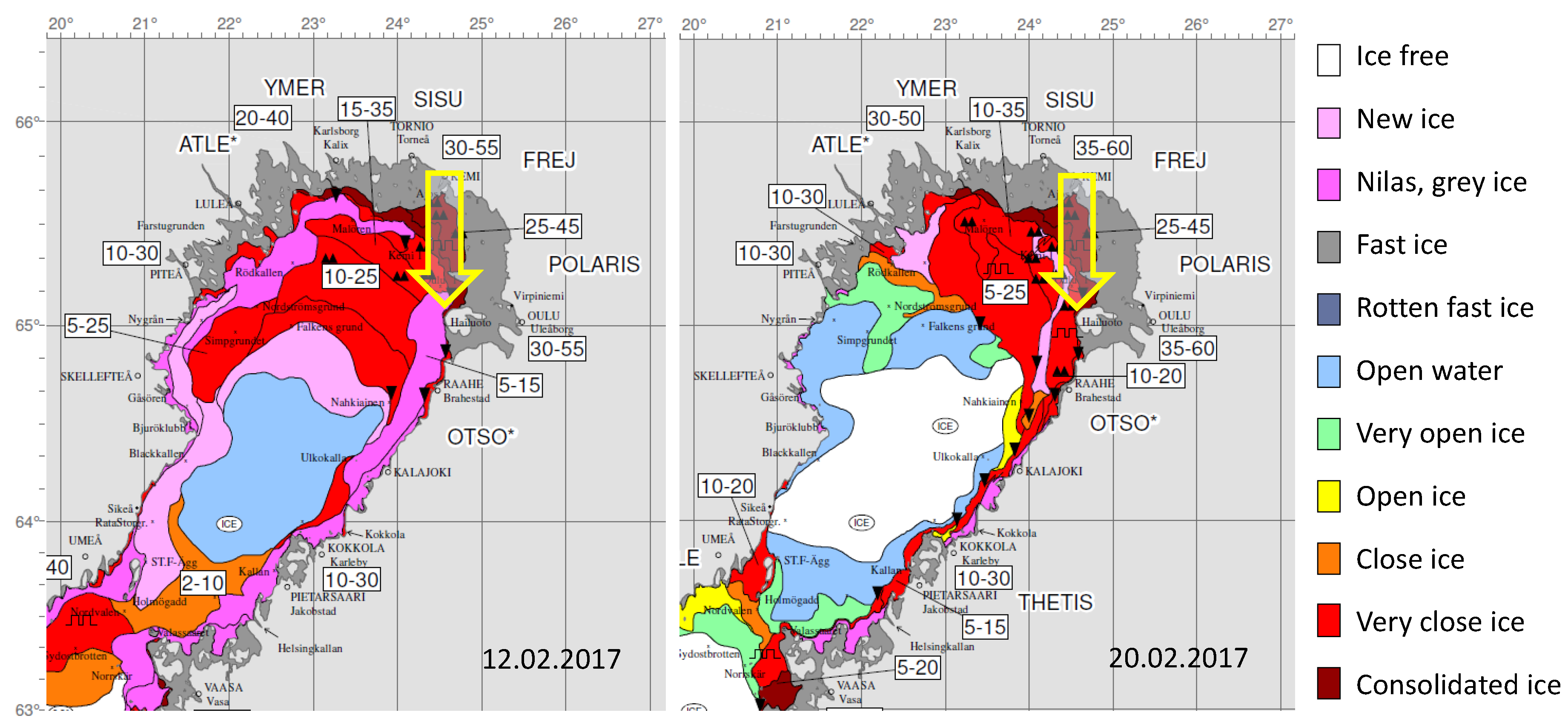
was observed on 12 February. At this time, Bothnian Bay was almost completely ice-covered by 10
to 25
thick drift ice, and the thickness of the land-fast ice was between 5
to 55
, as shown in
Figure 5 (left panel). In the middle of February, a westerly to northwesterly flow pattern strengthened over the region, causing dry and warm Föhn wind from the Scandinavian Mountains. Over Bothnian Bay, the ice field was packed against the Northeastern coast, and a large ice-free area in the center of the Bay formed (
Figure 5, right panel). Almost all ships to Oulu, Kemi, and Tornio had to be assisted by ice breakers. In the end of February, ice extent of the Baltic Sea was 77,000 km
.
On Hailuoto, the 2-m air temperature was 2
higher and the 10-m wind speed was
−1 lower than the climatological mean values for February during 1981–2010. In the first week of the ISOBAR campaign Hailuoto-I, from 11 to 18 February, the synoptic-scale conditions were characterized by a high-pressure center, first located over Southern Scandinavia and then moving over Central and Eastern Europe. Low pressure systems were passing over the North Atlantic, Norwegian Sea, and Barents Sea from southwest to northeast, resulting in variable winds, occasionally approaching 20
−1 in Hailuoto (
Figure 6). Depending on the air-mass origin, wind speed, and cloud cover, the 2-m air temperature in Hailuoto varied between −17
to 4
(
Figure 6). By 19 February, the high pressure center had moved north of the Azores, and a small low pressure system passed over Europe during 19 to 24 February. A passage of a warm front resulted in snow fall ( 8
water equivalent) on 23 February. From 24 to 27 February, the synoptic situation was dominated by two large low pressure systems, one first centered over Southern Finland, moving towards the northeast, and another one moving from the Denmark Strait to the Faroe Islands. In the saddle region between the lows, clear skies and weak winds allowed the 2-m air temperature, observed at the official weather station, to drop down to
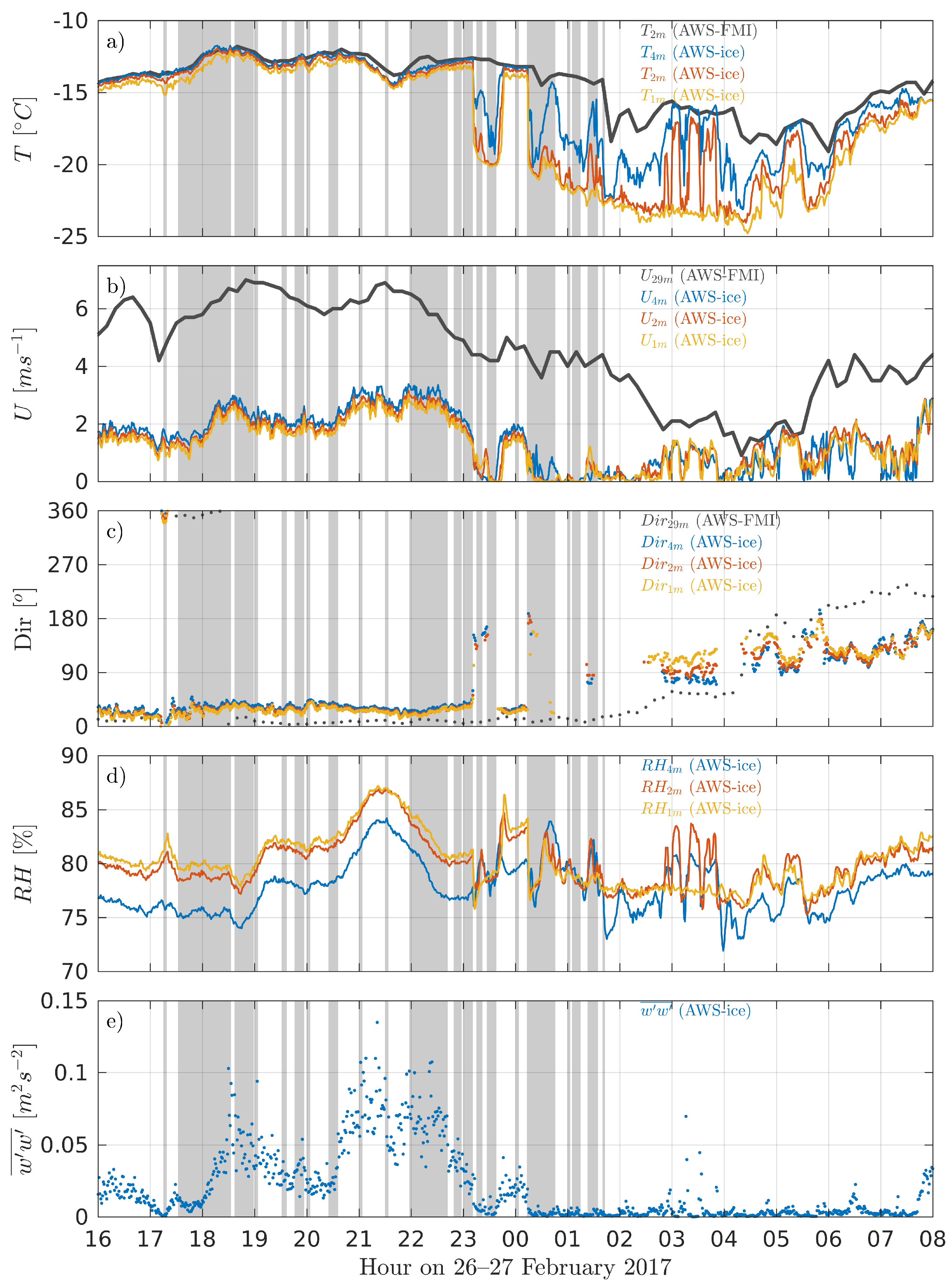
during the night of 27 February.
6. Summary and Outlook
The ISOBAR field campaign, Hailuoto-I, in February 2017 resulted in an extensive data set from several different observation systems, including ground-based in-situ and remote-sensing, in addition to airborne observations by various UAVs. The meteorological and sea ice conditions during the campaign did not represent the climatological means in the area with 2 higher temperatures and significantly less sea ice during most of February, compared to climatological references. Despite the relatively mild conditions, accompanied by a below average sea ice cover and the already significant diurnal cycle with notable short-wave radiation, a valuable data set on the SBL was sampled.
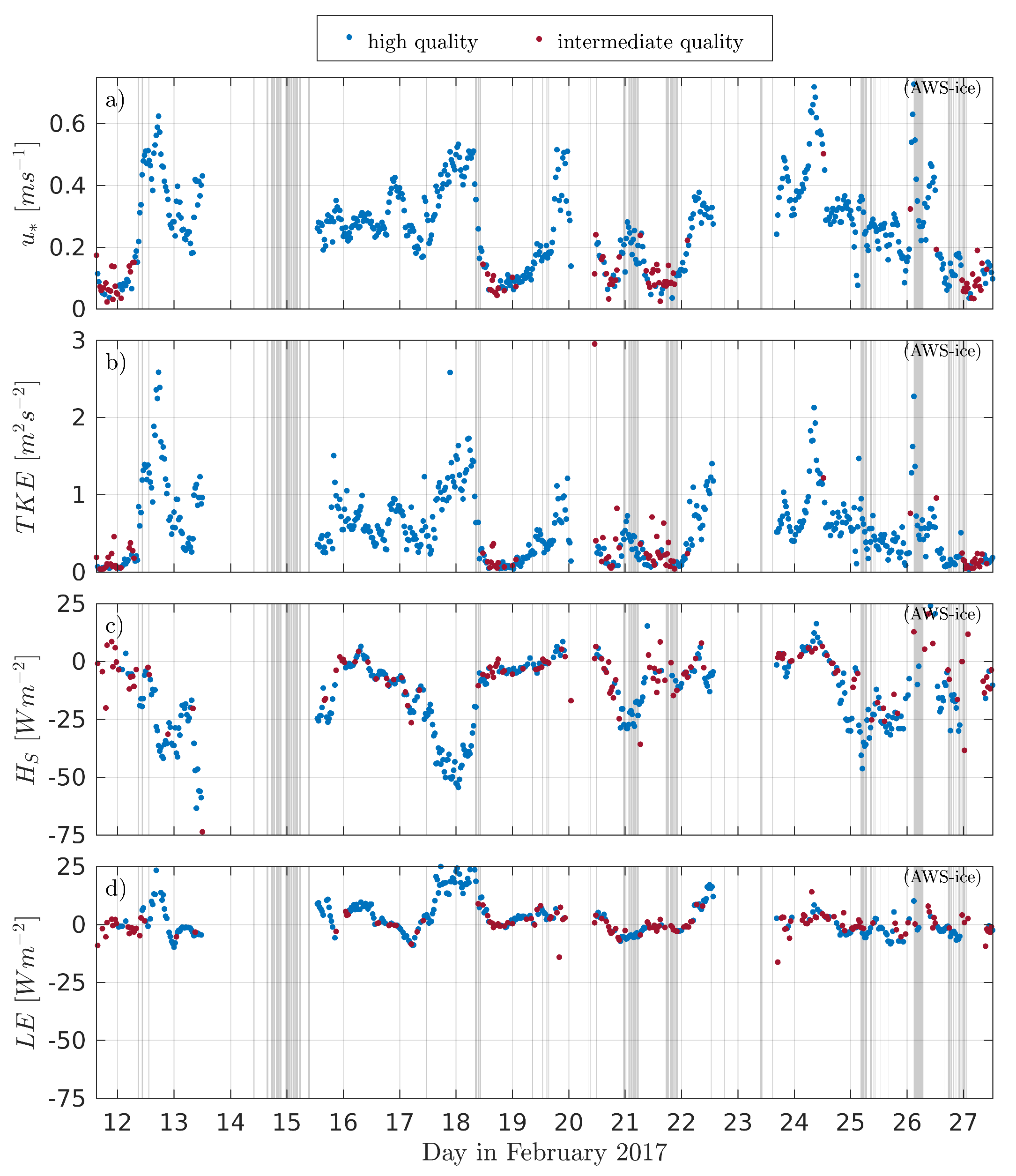
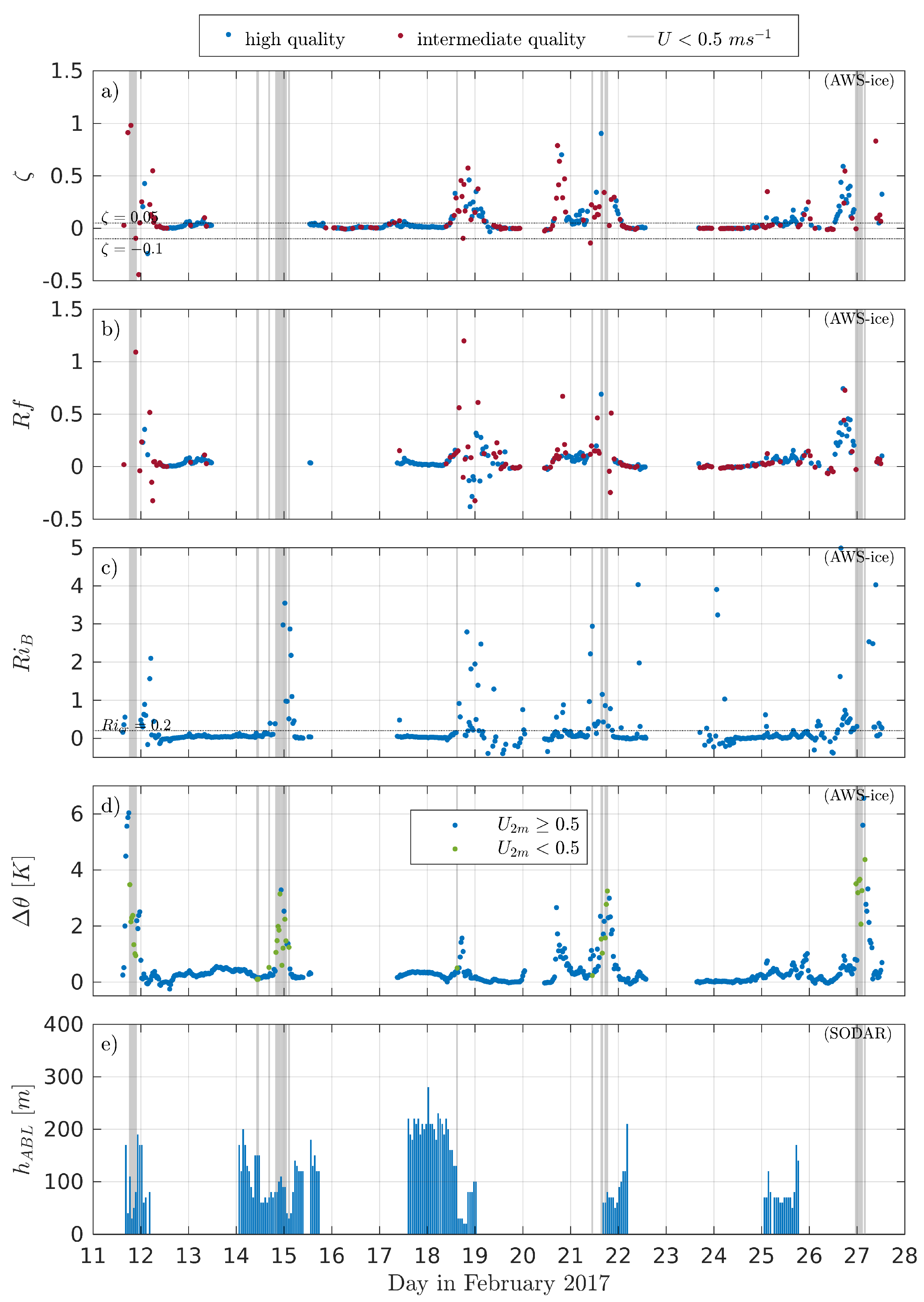
The stability of the SL was mostly near-neutral, but also, a fair amount of very-stable cases () occurred during the campaign, typically related to clear sky and weak wind or near-calm conditions. Under very stable conditions, the ABL height, , estimated from the SODAR data reached values as low as 20 . In general, wind shear seems to be a very important mechanism for creating turbulence. The long-wave upwelling radiation usually dominated over the other radiation terms and the turbulent fluxes of latent and sensible heat, with the latter also being significant.
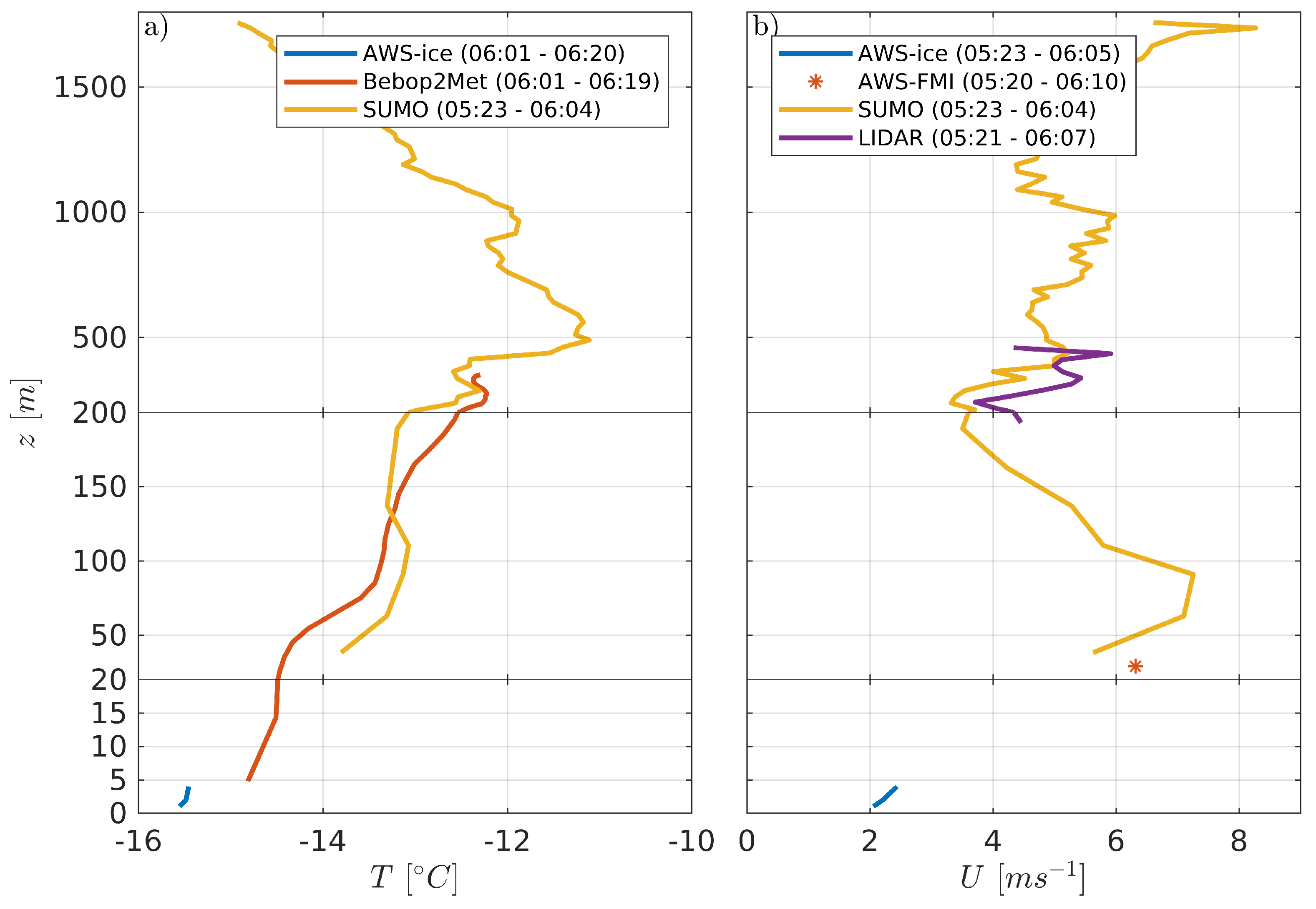
A unique approach was made in which data was combined from different profiling systems to create composite profiles, probing the atmospheric column from the surface to an altitude of 1800 agl with very high resolution in the lowermost layers. The agreement between the different systems was very good, given the systematic differences in the measurement principle, as well as in the vertical and temporal resolutions. Sampling the lowermost 200 or so repeatedly over several hours gave detailed information on the evolution of the SBL structure, such as a rapid cooling of the lowermost 20 and other relevant processes like warm air advection. The sampled data also contained at least one longer period of an SBL with very stable stratification and calm winds, which was characterized by a series of turbulent events leading to a rapid warming of the layers close to the ice surface. The UAV and SODAR profiling systems gave additional insight into the nature of these events, suggesting the existence of an elevated source of turbulence which could contribute to the occasional mixing events observed close to the surface.
The experience from this campaign motivated us to conduct a second, even more extensive field experiment. The ISOBAR campaign Hailuoto-II took place at the same site from 1 to 28 February 2018. The collected data from both ISOBAR field campaigns will be the basis for future SBL research studies. A particular focus will be on the combination of the observational data set with modeling approaches on different scales (NWP and LES) and with different levels of complexity (e.g., 3D and single column). The Weather Research and Forecasting (WRF) model [
2], run with different surface and boundary layer parameterization schemes, will be evaluated against the observations to better understand the physics and dynamics behind the observed events. For that purpose, we will also perform a series of experiments with the WRF model’s single-column mode, in which the atmospheric column above a single grid point from the 1
WRF domain is resolved with very high vertical resolution. This will give a deeper insight into the sensitivity of the SBL to changes in the prescribed surface conditions and model physics.
Accompanying the LES runs will be performed with the Parallelized Large-Eddy Simulation Model (PALM) [
99] to reveal SBL structure and dynamics, and virtual UAV measurements will be conducted on-the-fly during the simulation in order evaluate the representativeness of these measurements. The advantage in the LES is that the true state of the ABL is known, and errors induced by the measurement strategy can be directly evaluated. Based on the findings from this investigation, improved UAV flight strategies might be developed. Second, the problem of lacking grid convergence when simulating the SBL with LES will be addressed by applying a modified MOST-based surface boundary condition. Unlike existing boundary conditions, this will not lead to violations of the basic assumptions of MOST and inherent issues in LES modeling as outlined in the introduction. Finally, a series of LES runs shall be employed to evaluate both flux and alternative gradient-based similarity functions [
33,
34] in the SBL. This work will follow the methodology of the recent work for convective conditions by [
100] and will elucidate whether gradient-based similarity functions might be superior to the established flux-based MOST formulation, particularly under very stable conditions.

 ,
, 


