Impact of Subgrid-Scale Modeling in Actuator-Line Based Large-Eddy Simulation of Vertical-Axis Wind Turbine Wakes


Department of Engineering, Aarhus University, 8000 Aarhus C, Denmark
Atmosphere 2018, 9(7), 257; https://doi.org/10.3390/atmos9070257
Submission received: 24 June 2018
/
Revised: 6 July 2018
/
Accepted: 8 July 2018
/
Published: 10 July 2018
(This article belongs to the Special Issue Large-Eddy Simulations (LES) of Atmospheric Boundary Layer Flows)
Abstract
:A large-eddy simulation (LES) study of vertical-axis wind turbine wakes under uniform inflow conditions is performed. Emphasis is placed on exploring the effects of subgrid-scale (SGS) modeling on turbine loading as well as on the formation and development of the wind turbine wake. In this regard, the validated LES framework coupled with an actuator-line parametrization is employed. Three different SGS models are considered: the standard Smagorinsky model, the Lagrangian scale-dependent dynamic (LSDD) model, and the anisotropic minimum dissipation (AMD) model. The results show that the SGS model has a negligible effect on the mean aerodynamic loads acting on the blades. However, the structure of the wake, including the mean velocity and turbulence statistics, is significantly affected by the SGS closure. In particular, the standard Smagorisnky model with its theoretical model coefficient (i.e., ) postpones the transition of the wake to turbulence and yields a higher velocity variance in the turbulent region compared to the LSDD and AMD models. This observation is elaborated in more detail by analyzing the resolved-scale turbulent kinetic energy budget inside the wake. It is also shown that, unlike the standard Smagorinsky model, which requires detailed calibrations of the model coefficient, the AMD can yield predictions similar to the LSDD model for the mean and turbulence characteristics of the wake without any tuning.
1. Introduction
Power harvesting from atmospheric turbulent flows can be achieved through both horizontal-axis and vertical-axis wind turbines. Horizontal-axis wind turbines (HAWTs) are dominating the market, but vertical-axis wind turbines (VAWTs) have attracted renewed consideration in recent years due to their potential to provide a higher power output per unit land area [1]. This is, in part, because unlike for HAWTs, it is possible to increase the swept area of VAWTs independently of their footprints [2].
In addition to laboratory experiments [3,4,5,6,7,8,9,10,11] and field-scale measurements [2,12,13], numerical studies have also been performed in recent years to investigate the wake aerodynamics behind VAWTs [14,15,16,17,18,19]. Numerical simulations are a cost-effective approach that can provide detailed information about the fluid mechanics of VAWTs over a wide range of temporal and spatial scales. Specifically, large-eddy simulations (LES) coupled with a turbine model, such as the actuator-line technique, has become the leading numerical technique to simulate velocity and turbulence fields through wind turbines (see reviews by [20,21,22]). In the LES approach, turbulent structures larger than a certain filter width are resolved and the influence of the unresolved scales on the resolved motions are represented by a subgrid-scale (SGS) model. Hence, the accuracy of the LES can be affected by the performance of the SGS parametrization, especially in the anisotropic turbulence. It is of particular interest for wind energy applications to better understand and quantify how the SGS models affect the aerodynamic loads acting on the blades and also the formation and recovery of turbine wakes. This effect has been well studied and documented in the LES of HAWT wakes [23,24,25,26,27]. However, in the case of VAWTs, the role of SGS modeling on both the turbine loading and wake-flow structures has been studied less in prior investigations.
The present work aims to explore the effect of SGS modeling in LES on the turbine loading and flow characteristics of the wake downwind of a full-scale VAWT under uniform inflow conditions. The main reason for considering a uniform inflow condition in this study is that, in the absence of mean wind shear and turbulence in the incoming flow, the SGS model mainly controls the transition of the wake to turbulence [24,27]. Hence, this case will better assess the capability of different SGS models in capturing the point of transition and breakdown location of the wake. In this regard, the validated LES framework coupled with an actuator-line parametrization for the wind turbine is used [18]. A detailed description of the LES framework and the numerical setup are given in Section 2. The effects of SGS models on the aerodynamic loads as well as the spatial distribution of the mean and turbulence fields inside the wake are provided and discussed in Section 3. A detailed analysis of the resolved-scale turbulent kinetic energy (TKE) budget in the wake is presented in Section 4. Finally, concluding remarks are included in Section 5.
2. Large-Eddy Simulation Framework
2.1. LES Governing Equations
The LES framework utilized in this study is based on the filtered incompressible Navier–Stokes equations and the filtered continuity equation,
where the tilde indicates spatial filtering at the scale. is the fluid density. is instantaneous filtered velocity where corresponds to the streamwise (x), spanwise (y) and wall-normal (z) directions, respectively. t is time, is the filtered kinematic pressure, is the SGS stress tensor, and is an external body force corresponding to the effect of wind turbine on the flow. The viscous stress tensor based on filtered variables is defined as where is the fluid molecular viscosity, and is the resolved rate-of-strain tensor.
2.2. Subgrid-Scale Parametrization
In LES, the dynamics of the large-scale motions are computed explicitly, and the influence of the small-scale (or unresolved) structures on the large scales is parametrized using an SGS model [28]. An important category of SGS closures consists of eddy viscosity models which take into account the effect of small-scale eddies by locally increasing the molecular viscosity by means of an eddy viscosity. In this approach, the SGS stress tensor is represented as
where is the eddy viscosity. In this study, different SGS models were considered, all of them within the class of eddy-viscosity closures: the standard Smagorinsky model, the Lagrangian scale-dependent dynamic model, and the anisotropic minimum dissipation model. A short explanation of these models is provided in the following section.
2.2.1. Standard Smagorinsky Model
Using the mixing length approximation is one possible way to determine the eddy viscosity. This approximation yields the well-known Smagorinsky model [29]. In this approach, the eddy viscosity is formulated as
where is the Smagorinsky coefficient and . In the standard Smagorinsky model (denoted SMAG below), the model coefficient is assumed to be constant, independent of space and time. For the case of homogeneous isotropic turbulence with within the inertial subrange, an analysis performed by Lilly [30] using the spectral cut-off filter yielded . However, assuming a constant value for the model coefficient raises important concerns in the simulation of complex flows. In particular, for cases involving inhomogeneous and transitional flows, the general conclusion from a posteriori testing is that the standard Smagorinsky model is too dissipative; thus, the model coefficient should generally be decreased [28,31,32,33,34]. It follows that, in practice, and in order to yield acceptable results, the standard nondynamic approach requires detailed calibrations of the model coefficient [35,36]. Here, to assess the effect of Smagorinsky coefficient on wake flow structures, two values for the model coefficient were considered. The first one was the theoretical value proposed by Lilly [30] for isotropic turbulence (i.e., ) and the second one was the value used by Moin and Kim [32] for inhomogeneous channel flows (i.e., ).
2.2.2. Lagrangian Scale-Dependent Dynamic Smagorinsky Model
The dynamic procedure introduced by Germano et al. [37] provides a methodology to determine the appropriate local value of the Smagorinsky coefficient without any ad hoc tuning. In this approach, the Smagorinsky coefficient, which is space and time dependent, is computed by comparing the eddy dissipation at different scales. The dynamic model has been shown to improve SGS dissipation characteristics compared to the SMAG model [38,39,40]. In addition, the model appropriately switches off and does not yields extra eddy dissipation in laminar and transitional flow regions. However, an important assumption in the standard dynamic model is that the model coefficient is scale invariant. This assumption was later relaxed through the development of a scale-dependent dynamic model [35]. In this study, the Lagrangian scale-dependent dynamic (LSDD) model is employed where the model coefficient is computed dynamically and averaged along the fluid particle path [41]. Note that the computational complexity of the LSDD is much higher than that of the SMAG model. This results from performing the Lagrangian averaging procedure as well as the application of two test-filter operators. Specifically, as documented in [42], the application of the LSDD model increases the computational cost by about 35–40% over the SMAG model. More details about the LSDD closure can be found in [42].
2.2.3. Anisotropic Minimum Dissipation Model
Minimum dissipation models provide an alternative approach to specify the SGS stress tensor. They give the minimum amount of eddy dissipation needed to dissipate the energy of the subgrid scales. Verstappen [43] developed the first minimum dissipation model (called the QR model where Q and R represent the invariants of the resolved strain-rate tensor) for the eddy viscosity. The QR model yielded accurate results in simulations of turbulent flows with isotropic grids. Later, Rozema et al. [44] introduced the anisotropic minimum dissipation (AMD) model in which the properties of the QR model are generalized to anisotropic grids. The extension of the AMD closure to modeling the buoyancy-driven turbulent flows was recently done by Abkar et al. [45,46]. Among many desirable theoretical and practical properties of the AMD model, it appropriately switches off in laminar or transitional flow regions, and it is more cost-effective than the dynamic Smagorinsky approach. The AMD eddy-viscosity model is given by
where () is the scaled gradient operator, in which is a modified Poincaré constant, and is the grid size (Greek subscripts are excluded from the summation convention). Note that the modified Poincaré constant only depends on the order of accuracy of the discrete derivative operator in each direction, and its magnitude is independent of the size of the grid. In particular, the Poincaré constant is for second-order accurate schemes, and is equal to for spectral methods [44,47]. The AMD model showed robust performances in simulations of temporal mixing layers, decaying grid turbulence, and turbulent channel flow [44], in simulations of thermally stratified atmospheric boundary layers [45,46], and in simulations of VAWT wakes [18]. More details on the derivation of the AMD model for the SGS stress tensor can be found in [44,46].
2.3. Wind Turbine Parametrization
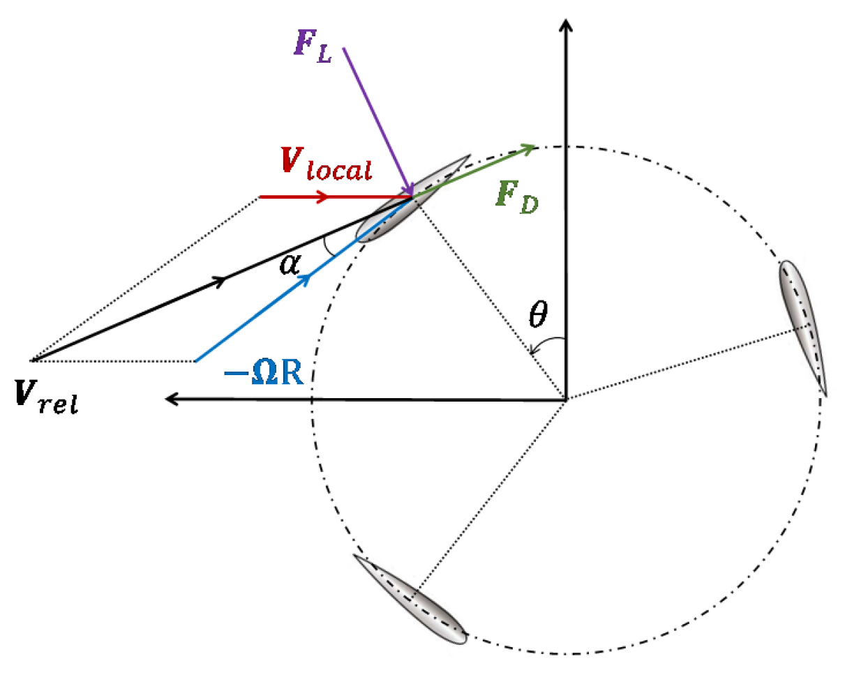
In this study, the actuator-line model was used to parametrize the turbine-induced forces. Through this approach, the drag and lift forces acting on the blades were computed using the blade element theory and applied along the lines which represent the blades of the turbine. In Figure 1, a horizontal cross-section of the blades is shown. Different velocities, angles, and forces are shown in this figure. is the turbine angular velocity, and R is the radius of the rotor. is the local velocity of the incident flow at the blade. is the angle of attack, and is the local velocity relative to the rotating blade. The turbine-induced force per unit vertical length of the blade is provided by
where and are the drag and lift coefficients, respectively; is the Reynolds number based on the chord length, c, and relative velocity, ; and denote the unit vectors in the directions of the drag and lift forces, respectively. The effect of dynamic stall on the drag and lift coefficients is taken into account using the modified MIT dynamic stall model [48]. This method has been successfully tested in recent studies focusing on modeling of VAWT wakes [10,14,15,18]. A tip-loss correction similar to the one proposed by Glauert [49] was also used in the blade element analysis. During the simulation, the local velocity at the blades was known. As a result, the local velocity relative to the rotating blades, , and the angle of attack, , could be calculated. The resulting forces were obtained using Equation (5). Note that, for numerical stability reasons, the applied blade forces were distributed smoothly over the actuator lines through the convolution of the computed force, , and a regularization kernel, [50], as
where d is the distance between the actuator-line and computational grid points, and is a parameter that controls how the forces are distributed onto the grids. The value of is typically in the range of 1–3 grid sizes [51]. In this study, it was set to times the grid size. The effect of the value on the simulation results was further assessed and is presented in Appendix A. Note that the present LES framework using the actuator-line technique has been validated against the laboratory data in the wake of a straight-bladed VAWT placed in the water channel [18].
2.4. Numerical Setup
The research code presented here has been developed and used in a series of wind energy studies (e.g., [52,53,54,55,56,57,58]). The numerical discretization follows the approach used by Moeng [59] and Albertson and Parlange [60] in which the computational domain is divided uniformly into , , and grid points in the x, y, and z directions, respectively. The governing equations (i.e., Equation (1)) are solved numerically using a pseudo-spectral discretization in the horizontal directions and a second-order finite difference scheme in the wall-normal direction. Aliasing errors are corrected in the nonlinear term using the 3/2 rule [61]. For time advancement, a second-order accurate Adams–Bashforth method is employed. The boundary conditions are periodic in the horizontal directions. Zero stress and zero vertical velocity conditions are imposed in the top and bottom boundaries.
In the simulations, a 200 kW VAWT with a rotor diameter (D) of 26 m was immersed in the flow. This particular turbine, which was designed and manufactured in collaboration with Uppsala University [62], is a straight bladed, Darrieus-type turbine. The rotor includes three straight blades with a span (H) of 24 m. A standard NACA 0018 airfoil with a chord length of about m was used for the blades [63]. Below the rated wind speed (∼12 m/s), the tip-speed ratio of the turbine was set to . The drag and lift coefficients of the blades were obtained from the tabulated airfoil data provided in [64]. The averaged Reynolds number based on the chord length and relative velocity was about for a tip-speed ratio of .
The domain sizes in the x, y, and z directions were set to , , and , respectively, and the simulations were performed with a grid resolution of . Note that the grid resolution sensitivity of the numerical results was tested and is provided in the Appendix A. The turbine was placed at three rotor diameters downstream from the inflow in the center of the plane. The incoming wind to the turbine was uniform with a velocity of m/s. To adjust the flow from the downstream wake state to an undisturbed inflow condition, a fringe zone upstream of the turbine was used. In this method, the downstream wake flow does not affect the inflow condition due to the imposed periodic boundary conditions [65,66,67,68]. The simulations were initially run for two flow throughs to guarantee that quasi-steady conditions were achieved, and then the quantities of interest were averaged over three flow throughs.
3. Results
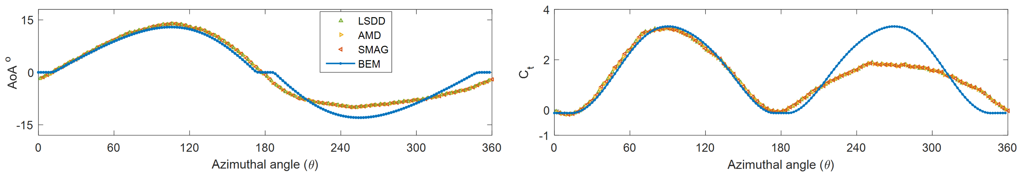
Figure 2 shows the time-averaged values of the angle of attack and the tangential force coefficient versus the azimuthal angle, respectively. The results obtained from the blade element momentum (BEM) theory are also shown for comparison. Note that the BEM theory equations were derived from momentum and blade element theories and are solved iteratively [69]. As can be seen in these figures, there was good agreement between the LES simulations and the BEM theory in the first half of the blade revolution. However, there was a discrepancy between the LES and the BEM theory in the second half of the blade revolution. This is mainly because in the second half of the revolution, the blades are in the wake generated by the other blades in the upstream. Since the reference velocity used in the BEM theory is independent of the blade locations, this approach is not able to correctly predict the aerodynamic loads in the second half of the blade revolution. These figures also reveal that the SGS model negligibly affects the mean aerodynamic loads acting on the blades and the predictions of all SGS models lay on top of each other.
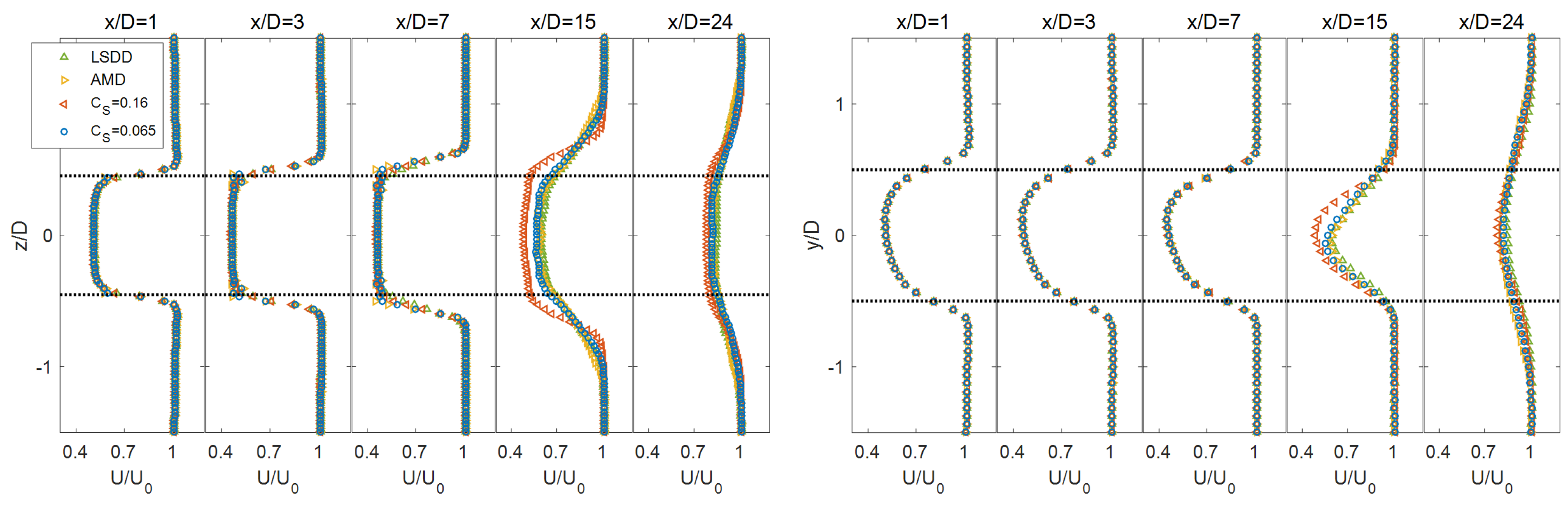
Figure 3 displays the contours of mean streamwise velocity in the central vertical and horizontal planes through the turbine equator. Note that the wake generated behind the turbine gradually recovers with distance as faster moving fluid is entrained in the wake. The asymmetry of the wake in the horizontal plane can also be observed in this figure which is the inherent characteristic of VAWT wakes and is mainly related to the rotation of the turbine. Similar behavior has been reported in previous numerical and experimental studies of the wake of VAWTs [3,5,8,17,70,71,72,73]. The vertical and lateral profiles of the mean streamwise velocity at the turbine equator are also plotted in Figure 4 for five different downstream locations at , 3, 7, 15 and 24. It can be visually acknowledged that the flow fields predicted by all the SGS models are similar in the region close to the turbine. The differences between the profiles are observed at locations where the turbulence is trigged and the wake starts breaking down. In particular, the SMAG model with the theoretical value for the Smagorisnky coefficient () postpones the breakdown location of the wake. This is most likely because the model is too dissipative and damps the small-scale turbulence that causes the instability of the wake [26,27]. It was also found that the AMD model can provide comparable results to the LSDD model for predicting the wake velocity. Note that the computational complexity of AMD is much lower than LSDD, and it is comparable to the SMAG model. Additionally, it was realized that decreasing the model coefficient in the SMAG approach to improves the mean velocity predictions in the vicinity of the breakdown location of the wake.
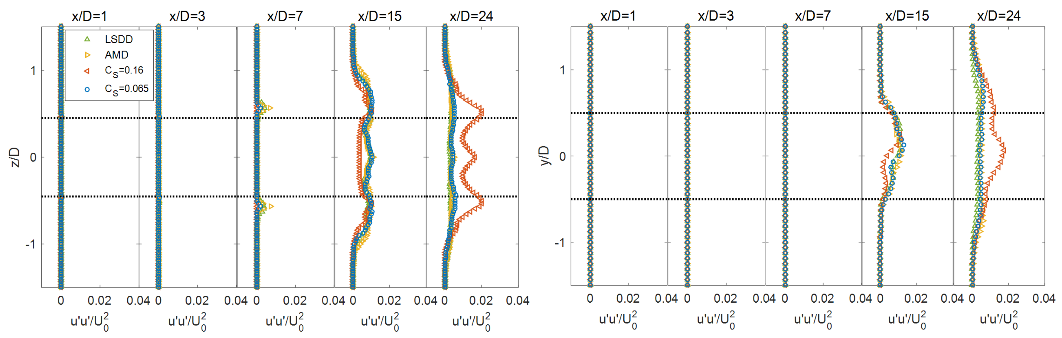
Figure 5 shows the contour plots of normalized streamwise velocity variance in the central vertical and horizontal planes through the turbine. Here, the overbar denotes temporal averaging, and . The lateral and vertical profiles of this quantity through the center of the turbine are also plotted in Figure 6. It can be observed that in the near wake region in which the turbulence is not triggered yet, the velocity variance is almost zero. At some distance downwind from the turbine where the turbulence is triggered, an apparent enhancement of turbulent fluctuations is observed. Specifically, a higher turbulence intensity is observed at the top and bottom edges and close to the two side-tip positions of the turbine, which is mainly caused by the strong shear at these locations [15]. It can also be observed that, in the horizontal plane, the turbulence level is stronger in the upcoming blade region which is connected to stronger shear in that area compared to the retreating blade region. These figures also investigate the effect of the SGS model on the wake formation and breakdown. It can be understood from these figures that the location at which the transition of the wake to turbulence occurs is affected by the SGS closure. Consistent with the previous results for the mean velocity profiles, the SMAG model with delays the point of transition which is due to the fact that the model is highly dissipative [27]. Note that unlike the mean velocity profiles, in which the predictions of different SGS models are similar in the far wake region, the discrepancies in the velocity variance profiles are larger and clearly visible at locations further downstream of the wake breakdown. It is also interesting to observe that despite the fact that the SMAG model with is too dissipative, the turbulence level in the far wake is higher for that model than for the other cases which are less dissipative. This observation is investigated in more detail in the next section by performing the resolved-scale TKE budget analysis. Again, it can be noticed that the results obtained from the AMD model are comparable with the ones obtained from the LSDD model. Also, similar to the presented results for the mean velocity distribution, reducing the model coefficient in the SMAG model can improve the prediction of the turbulence properties in the far-wake region.
4. Resolved-Scale Turbulent Kinetic Energy Budget
As shown in Figure 5, the turbulence level in the far-wake is larger for the SMAG model with than for the other cases. To better understand the role of the SGS closure on the energy exchanges between the resolved and the SGS parts, a detailed analysis of the resolved-scale TKE budget in the wake was carried out. The resolved-scale TKE budget equation can be expressed as [74]
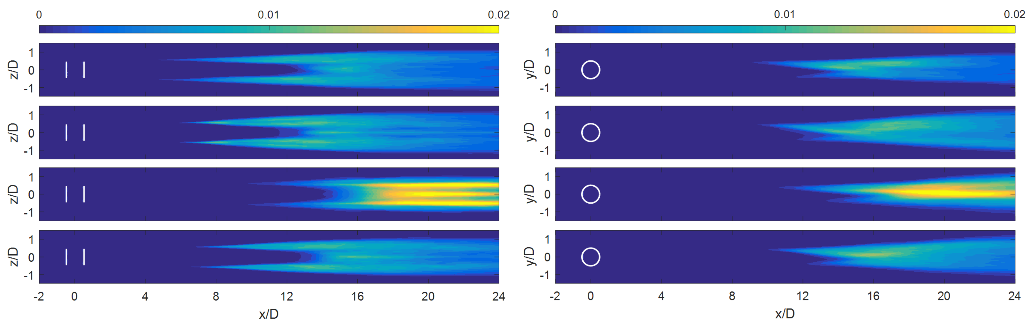
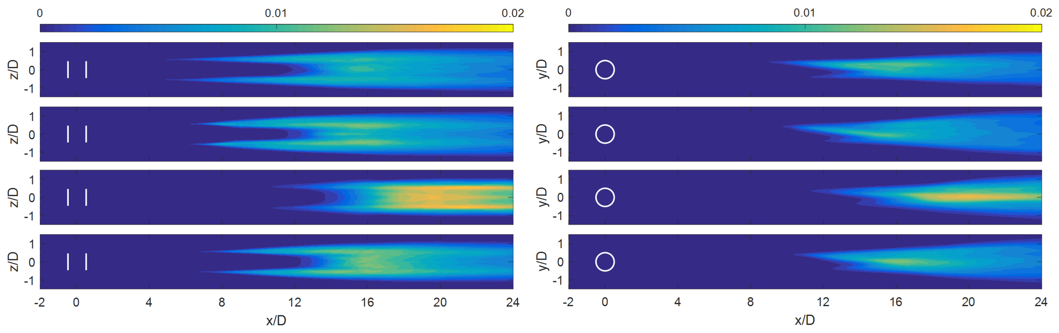
where denotes the mean resolved-scale TKE. , , , and represent the transport of the resolved-scale TKE with velocity, pressure, viscous stress fluctuations, and SGS stress fluctuations, respectively. is the shear production describing the conversion of the mean kinetic energy to the resolved-scale TKE, is the rate of the work against the turbine-induced forces, is the viscous dissipation rate of the resolved-scale TKE, and is the SGS dissipation rate and represents the energy transfer from the resolved scales to the subgrid scales. In this study, the focus was placed only on the last term on the right-hand side of the above-mentioned equation to investigate the contribution of the SGS closure on the energy exchange between the resolved and subgrid scales. Figure 7 displays the two-dimensional contours of the SGS dissipation rate obtained from the application of different SGS closures. It was observed that the SGS dissipation rate inside the wake is strongly affected by the SGS model, and in the particular cases considered here, it was lower for the SMAG model with than for the other models. A possible explanation for this observation is that the energy transfer between the resolved scales is flawed in the SMAG model with , and that leads to the accumulation of kinetic energy in the resolved part and consequently, to a higher velocity variance in the turbulent region of the wake (shown in Figure 5). It is worth mentioning here that similar behavior was reported recently in the study by Martinez-Tossas et al. [27] in the simulation of HAWT wakes under uniform inflow. To justify this trend, they argued that enhances the damping of the smallest resolved turbulent eddies which, in turn, disrupts the natural energy cascade and leads to the augmentation of TKE in the resolved part. The results of the TKE distribution in the wake are displayed in Figure 8.
5. Conclusions
The validated LES framework coupled with the actuator-line method was employed to investigate the impact of SGS modeling on the turbine loading as well as the formation and recovery of the wake behind a full-scale VAWT in uniform inflow. Three different SGS models were considered: the standard Smagorinsky (SMAG) model with two different values for the model coefficient, the Lagrangian scale-dependent dynamic (LSDD) model, and the anisotropic minimum dissipation (AMD) model.
The simulation results show that the influence of SGS models on the mean aerodynamic loads on the blades is negligible. However, the SGS model has a significant impact on the distribution of the wake velocity and turbulence statistics downwind of the turbine. In particular, the SMAG model with its theoretical value (i.e., ) postpones the transition of the wake to turbulence to a distance further downstream and produces a higher turbulence intensity in that region compared to the LSDD and AMD models. A detailed analysis of the resolved-scale TKE budget in the wake region also revealed that the SMAG model with overdissipates the energy of the smallest resolved scales. This, in turn, reduces the the natural energy transfer from the resolved to subgrid scales and consequently, leads to the accumulation of TKE in the resolved part [27]. It was also shown that calibrating the model coefficient in the SMAG model (i.e., in this study) can improve the prediction of the turbulence statistics as well as the breakdown location of the wake. However, the AMD model can yield acceptable results similar to the LSDD model for the mean and turbulence characteristics in the wake without any tuning and with low computational complexity.
Funding
This research received no external funding.
Acknowledgments
This paper benefited from comments by Prof. Parviz Moin. The computational resources used in this study were provided by the Center for Turbulence Research (CTR) at Stanford University.
Conflicts of Interest
The author declares no conflict of interest.
Appendix A. Effects of the Smearing Parameter and Grid Resolution
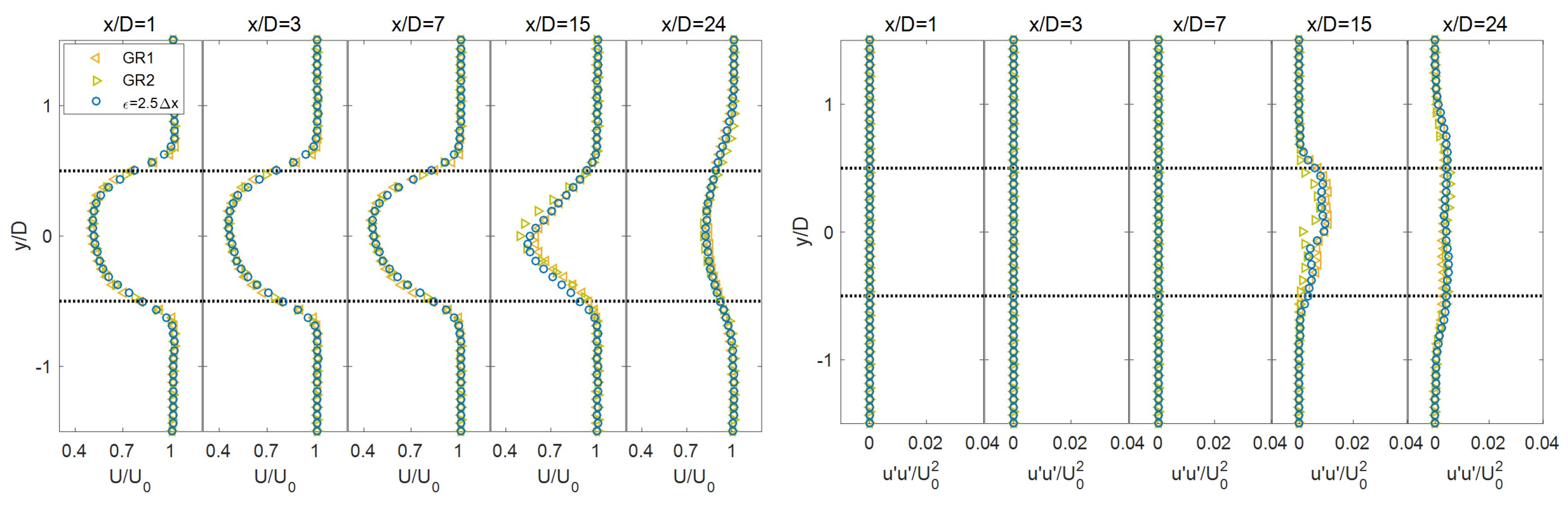
As mentioned in Section 2.3, for the sake of numerical stability, the applied blade forces were smoothly distributed through the actuator lines. In the application of the actuator-line model, a value in the order of grid sizes is recommended for the smearing parameter () shown in Equation (6) [51,75]. In order to study the sensitivity of the numerical results to the smearing parameter, numerical experiments were performed with two different values both within the recommended range: and . The lateral profiles of the normalized mean velocity and streamwise velocity variance obtained from the LSDD model with two different values are shown in Figure A1. As can be noticed from this figure, for the particular cases considered in this study, the profiles of the mean velocity and velocity variance showed very little dependence on the smearing parameter.
Also, in order to further evaluate the sensitivity of the simulation results to the grid resolution, the results obtained from the LSDD model with two different grids which are of sizes GR1 () and GR2 () in the x, y, and z directions, respectively, were compared. In the simulations, similar cell aspect ratios were used (:: ≈ 2:2:1). Figure A1 also illustrates the lateral profiles of the normalized mean velocity and streamwise velocity variance obtained from the two different grid resolutions. As can be seen in this figure, there was a very small grid resolution dependence in the profiles of the mean velocity and streamwise velocity variance, especially in the far wake region at , where the impact of the SGS model on the turbulence level was stronger.
Figure A1.
Lateral profiles of the normalized streamwise velocity () (left) and streamwise velocity variance () (right) through the hub level at downwind of the turbine obtained from the LSDD model with two different values and two different spatial resolutions.
Figure A1.
Lateral profiles of the normalized streamwise velocity () (left) and streamwise velocity variance () (right) through the hub level at downwind of the turbine obtained from the LSDD model with two different values and two different spatial resolutions.

References
- Araya, D.B.; Craig, A.E.; Kinzel, M.; Dabiri, J.O. Low-order modeling of wind farm aerodynamics using leaky Rankine bodies. J. Renew. Sustain. Energy 2014, 6, 063118. [Google Scholar] [CrossRef] [Green Version]
- Dabiri, J.O. Potential order-of-magnitude enhancement of wind farm power density via counter-rotating vertical-axis wind turbine arrays. J. Renew. Sustain. Energy 2011, 3, 043104. [Google Scholar] [CrossRef] [Green Version]
- Battisti, L.; Zanne, L.; Dell’Anna, S.; Dossena, V.; Persico, G.; Paradiso, B. Aerodynamic Measurements on a Vertical Axis Wind Turbine in a Large Scale Wind Tunnel. J. Energy Resour. Technol. 2011, 133, 031201. [Google Scholar] [CrossRef]
- Bachant, P.; Wosnik, M. Characterising the near-wake of a cross-flow turbine. J. Turbul. 2015, 16, 392–410. [Google Scholar] [CrossRef]
- Araya, D.B.; Dabiri, J.O. A comparison of wake measurements in motor-driven and flow-driven turbine experiments. Exp. Fluids 2015, 56, 1–15. [Google Scholar] [CrossRef]
- Posa, A.; Parker, C.M.; Leftwich, M.C.; Balaras, E. Wake structure of a single vertical axis wind turbine. Int. J. Heat Fluid Flow 2016. [Google Scholar] [CrossRef]
- Ryan, K.J.; Coletti, F.; Elkins, C.J.; Dabiri, J.O.; Eaton, J.K. Three-dimensional flow field around and downstream of a subscale model rotating vertical axis wind turbine. Exp. Fluids 2016, 57, 1–15. [Google Scholar] [CrossRef]
- Araya, D.B.; Colonius, T.; Dabiri, J.O. Transition to bluff-body dynamics in the wake of vertical-axis wind turbines. J. Fluid Mech. 2017, 813, 346–381. [Google Scholar] [CrossRef]
- Craig, A.E.; Dabiri, J.O.; Koseff, J.R. Low order physical models of vertical axis wind turbines. J. Renew. Sustain. Energy 2017, 9, 013306. [Google Scholar] [CrossRef] [Green Version]
- Rolin, V.; Porté-Agel, F. Experimental investigation of vertical-axis wind-turbine wakes in boundary layer flow. Renew. Energy 2018, 118, 1–13. [Google Scholar] [CrossRef]
- Kadum, H.; Friedman, S.; Camp, E.H.; Cal, R.B. Development and scaling of a vertical axis wind turbine wake. J. Wind Eng. Ind. Aerodyn. 2018, 174, 303–311. [Google Scholar] [CrossRef]
- Kinzel, M.; Mulligan, Q.; Dabiri, J.O. Energy exchange in an array of vertical-axis wind turbines. J. Turbul. 2012, 13, 1–13. [Google Scholar] [CrossRef]
- Brownstein, I.D.; Kinzel, M.; Dabiri, J.O. Performance enhancement of downstream vertical-axis wind turbines. J. Renew. Sustain. Energy 2016, 8, 053306. [Google Scholar] [CrossRef] [Green Version]
- Shamsoddin, S.; Porté-Agel, F. Large Eddy Simulation of Vertical Axis Wind Turbine Wakes. Energies 2014, 7, 890–912. [Google Scholar] [CrossRef] [Green Version]
- Shamsoddin, S.; Porté-Agel, F. A Large-Eddy Simulation Study of Vertical Axis Wind Turbine Wakes in the Atmospheric Boundary Layer. Energies 2016, 9, 366. [Google Scholar] [CrossRef]
- Lam, H.; Peng, H. Study of wake characteristics of a vertical axis wind turbine by two-and three-dimensional computational fluid dynamics simulations. Renew. Energy 2016, 90, 386–398. [Google Scholar] [CrossRef]
- Hezaveh, S.H.; Bou-Zeid, E.; Lohry, M.W.; Martinelli, L. Simulation and wake analysis of a single vertical axis wind turbine. Wind Energy 2016, 20, 713–730. [Google Scholar] [CrossRef]
- Abkar, M.; Dabiri, J.O. Self-similarity and flow characteristics of vertical-axis wind turbine wakes: An LES study. J. Turbul. 2017, 18, 373–389. [Google Scholar] [CrossRef]
- Rezaeiha, A.; Kalkman, I.; Montazeri, H.; Blocken, B. Effect of the shaft on the aerodynamic performance of urban vertical axis wind turbines. Energy Convers. Manag. 2017, 149, 616–630. [Google Scholar] [CrossRef]
- Mehta, D.; Van Zuijlen, A.; Koren, B.; Holierhoek, J.; Bijl, H. Large eddy simulation of wind farm aerodynamics: A review. J. Wind Eng. Ind. Aerodyn. 2014, 133, 1–17. [Google Scholar] [CrossRef]
- Stevens, R.J.; Meneveau, C. Flow structure and turbulence in wind farms. Ann. Rev. Fluid Mech. 2017, 49, 311–339. [Google Scholar] [CrossRef]
- Breton, S.P.; Sumner, J.; Sørensen, J.N.; Hansen, K.S.; Sarmast, S.; Ivanell, S. A survey of modelling methods for high-fidelity wind farm simulations using large eddy simulation. Phil. Trans. R. Soc. A 2017, 375, 20160097. [Google Scholar] [CrossRef] [PubMed] [Green Version]
- Wu, Y.T.; Porté-Agel, F. Large-Eddy Simulation of Wind-Turbine Wakes: Evaluation of Turbine Parametrisations. Bound.-Lay. Meteorol. 2011, 138, 345–366. [Google Scholar] [CrossRef]
- Sarlak, H.; Meneveau, C.; Sørensen, J.N. Role of subgrid-scale modeling in large eddy simulation of wind turbine wake interactions. Renew. Energy 2015, 77, 386–399. [Google Scholar] [CrossRef]
- Sarlak, H.; Meneveau, C.; Sørensen, J.N.; Mikkelsen, R. Quantifying the impact of subgrid scale models in actuator-line based LES of wind turbine wakes in laminar and turbulent inflow. In Direct and Large-Eddy Simulation IX; Springer: Berlin, Germany, 2015; pp. 169–175. [Google Scholar]
- Martínez-Tossas, L.A.; Churchfield, M.J.; Meneveau, C. Large eddy simulation of wind turbine wakes: Detailed comparisons of two codes focusing on effects of numerics and subgrid modeling. J. Phys. Conf. Ser. 2015, 625, 012024. [Google Scholar] [CrossRef]
- Martínez-Tossas, L.A.; Churchfield, M.J.; Yilmaz, A.E.; Sarlak, H.; Johnson, P.L.; Sørensen, J.N.; Meyers, J.; Meneveau, C. Comparison of four large-eddy simulation research codes and effects of model coefficient and inflow turbulence in actuator-line-based wind turbine modeling. J. Renew. Sustain. Energy 2018, 10, 033301. [Google Scholar] [CrossRef] [Green Version]
- Pope, S. Turbulent Flows; Cambridge University Press: Cambridge, UK, 2000. [Google Scholar]
- Smagorinsky, J. General Circulation Experiments with the Primitive Equations. Mon. Weather Rev. 1963, 91, 99–164. [Google Scholar] [CrossRef]
- Lilly, D.K. The representation of small-scale turbulence in numerical simulation experiments. In Proceedings of the IBM Scientific Computing Symposium on Environmental Sciences, Yorktown Height, NY, USA, 4–16 November 1966; p. 167. [Google Scholar]
- Deardorff, J.W. A numerical study of three-dimensional turbulent channel flow at large Reynolds numbers. J. Fluid Mech. 1970, 41, 453–480. [Google Scholar] [CrossRef]
- Moin, P.; Kim, J. Numerical investigation of turbulent channel flow. J. Fluid Mech. 1982, 118, 341–377. [Google Scholar] [CrossRef]
- Piomelli, U.; Moin, P.; Ferziger, J.H. Model consistency in large eddy simulation of turbulent channel flows. Phys. Fluids 1988, 31, 1884–1891. [Google Scholar] [CrossRef]
- Vreman, B.; Geurts, B.; Kuerten, H. Large-eddy simulation of the turbulent mixing layer. J. Fluid Mech. 1997, 339, 357–390. [Google Scholar] [CrossRef] [Green Version]
- Porté-Agel, F.; Meneveau, C.; Parlange, M.B. A Scale-Dependent Dynamic Model for Large-Eddy Simulation: Application to a Neutral Atmospheric Boundary Layer. J. Fluid Mech. 2000, 415, 261–284. [Google Scholar] [CrossRef]
- Bou-Zeid, E.; Meneveau, C.; Parlange, M. A scale-dependent Lagrangian dynamic model for large eddy simulation of complex turbulent flows. Phys. Fluids 2005, 17, 025105. [Google Scholar] [CrossRef] [Green Version]
- Germano, M.; Piomelli, U.; Moin, P.; Cabot, W. A dynamic subgrid-scale eddy viscosity model. Phys. Fluids 1991, 3, 1760–1765. [Google Scholar] [CrossRef]
- Piomelli, U. High Reynolds number calculations using the dynamic subgrid-scale stress model. Phys. Fluids A 1993, 5, 1484–1490. [Google Scholar] [CrossRef]
- Meneveau, C.; Katz, J. Scale-invariance and turbulence models for large-eddy simulation. Ann. Rev. Fluid Mech. 2000, 32, 1–32. [Google Scholar] [CrossRef]
- Khani, S.; Waite, M.L. Large eddy simulations of stratified turbulence: The dynamic Smagorinsky model. J. Fluid Mech. 2015, 773, 327–344. [Google Scholar] [CrossRef]
- Meneveau, C.; Lund, T.S.; Cabot, W.H. A Lagrangian dynamic subgrid-scale model of turbulence. J. Fluid Mech. 1996, 319, 353–385. [Google Scholar] [CrossRef] [Green Version]
- Stoll, R.; Porté-Agel, F. Dynamic subgrid-scale models for momentum and scalar fluxes in large-eddy simulations of neutrally stratified atmospheric boundary layers over heterogeneous terrain. Water Resour. Res. 2006, 42, W01409. [Google Scholar] [CrossRef]
- Verstappen, R. When does eddy viscosity damp subfilter scales sufficiently? J. Sci. Comput. 2011, 49, 94–110. [Google Scholar] [CrossRef]
- Rozema, W.; Bae, H.J.; Moin, P.; Verstappen, R. Minimum-dissipation models for large-eddy simulation. Phys. Fluids 2015, 27, 085107. [Google Scholar] [CrossRef] [Green Version]
- Abkar, M.; Bae, H.; Moin, P. Minimum-dissipation scalar transport model for large-eddy simulation of turbulent flows. Phys. Rev. Fluids 2016, 1, 041701. [Google Scholar] [CrossRef]
- Abkar, M.; Moin, P. Large-Eddy Simulation of Thermally Stratified Atmospheric Boundary-Layer Flow Using a Minimum Dissipation Model. Bound.-Lay. Meteorol. 2017, 165, 405–419. [Google Scholar] [CrossRef]
- Verstappen, R.; Rozema, W.; Bae, H. Numerical scale separation in large-eddy simulation. In Proceedings of the Summer Program 2014, Stanford, CA, USA, 6 July–1 August 2014; pp. 417–426. [Google Scholar]
- Noll, R.B.; Ham, N.D. Dynamic Stall of small Wind Systems; Technical Report; Aerospace Systems Inc.: Burlington, MA, USA, 1983. [Google Scholar]
- Glauert, H. Airplane propellers. In Aerodynamic Theory; Durand, W.F., Ed.; Dover Publications: Mineola, NY, USA, 1963; pp. 169–360. [Google Scholar]
- Sørensen, J.N.; Shen, W.Z. Numerical modeling of wind turbine wakes. J. Fluid Eng. 2002, 124, 393–399. [Google Scholar] [CrossRef]
- Troldborg, N.; Sørensen, J.; Mikkelsen, R. Actuator line simulation of wake of wind turbine operating in turbulent inflow. J. Phys. Conf. Ser. 2007, 75, 012063. [Google Scholar] [CrossRef]
- Porté-Agel, F.; Wu, Y.T.; Lu, H.; Conzemius, R.J. Large-eddy simulation of atmospheric boundary layer flow through wind turbines and wind farms. J. Wind Eng. Ind. Aerodyn. 2011, 99, 154–168. [Google Scholar] [CrossRef]
- Wu, Y.T.; Porté-Agel, F. Simulation of Turbulent Flow Inside and Above Wind Farms: Model Validation and Layout Effects. Bound.-Lay. Meteorol. 2013, 146, 181–205. [Google Scholar] [CrossRef]
- Abkar, M.; Porté-Agel, F. The Effect of Free-Atmosphere Stratification on Boundary-Layer Flow and Power Output from Very Large Wind Farms. Energies 2013, 6, 2338–2361. [Google Scholar] [CrossRef] [Green Version]
- Abkar, M.; Porté-Agel, F. Mean and turbulent kinetic energy budgets inside and above very large wind farms under conventionally-neutral condition. Renew. Energy 2014, 70, 142–152. [Google Scholar] [CrossRef]
- Abkar, M.; Porté-Agel, F. A new wind-farm parameterization for large-scale atmospheric models. J. Renew. Sustain. Energy 2015, 7, 013121. [Google Scholar] [CrossRef]
- Abkar, M.; Porté-Agel, F. Influence of the Coriolis force on the structure and evolution of wind turbine wakes. Phys. Rev. Fluids 2016, 1, 063701. [Google Scholar] [CrossRef]
- Yang, X.I.; Abkar, M. A hierarchical random additive model for passive scalars in wall-bounded flows at high Reynolds numbers. J. Fluid Mech. 2018, 842, 354–380. [Google Scholar] [CrossRef]
- Moeng, C. A large-eddy simulation model for the study of planetary boundary-layer turbulence. J. Atmos. Sci. 1984, 46, 2311–2330. [Google Scholar] [CrossRef]
- Albertson, J.D.; Parlange, M.B. Surfaces length scales and shear stress: Implications for land-atmosphere interactions over complex terrain. Water Resour. Res. 1999, 35, 2121–2132. [Google Scholar] [CrossRef]
- Canuto, C.; Hussaini, M.; Quarteroni, A.; Zang, T. Spectral Methods in Fluid Dynamics; Springer: Berlin, Germany, 1988. [Google Scholar]
- Möllerström, E.; Ottermo, F.; Hylander, J.; Bernhoff, H. Noise Emission of a 200 kW Vertical Axis Wind Turbine. Energies 2015, 9, 19. [Google Scholar] [CrossRef]
- Möllerström, E.; Ottermo, F.; Goude, A.; Eriksson, S.; Hylander, J.; Bernhoff, H. Turbulence influence on wind energy extraction for a medium size vertical axis wind turbine. Wind Energy 2016, 19, 1963–1973. [Google Scholar] [CrossRef]
- Sheldahl, R.E.; Klimas, P.C. Aerodynamic Characteristics of Seven Airfoil Sections through 180 Degrees Angle of Attack for Use in Aerodynamic Analysis of Vertical Axis Wind Turbines; Technical Report SAND80-2114; Sandia National Laboratories: Livermore, CA, USA, 1981. [Google Scholar]
- Tseng, Y.H.; Meneveau, C.; Parlange, M.B. Modeling flow around bluff bodies and predicting urban dispersion using large eddy simulation. Environ. Sci. Technol. 2006, 40, 2653–2662. [Google Scholar] [CrossRef] [PubMed]
- Abkar, M.; Porté-Agel, F. A new boundary condition for large-eddy simulation of boundary-layer flow over surface roughness transitions. J. Turbul. 2012, 13, 1–18. [Google Scholar] [CrossRef]
- Munters, W.; Meneveau, C.; Meyers, J. Turbulent Inflow Precursor Method with Time-Varying Direction for Large-Eddy Simulations and Applications to Wind Farms. Bound.-Lay. Meteorol. 2016, 159, 305–328. [Google Scholar] [CrossRef] [Green Version]
- Abkar, M.; Sharifi, A.; Porté-Agel, F. Wake flow in a wind farm during a diurnal cycle. J. Turbul. 2016, 17, 420–441. [Google Scholar] [CrossRef]
- Manwell, J.F.; McGowan, J.G.; Rogers, A.L. Wind Energy Explained: Theory, Design and Application; John Wiley & Sons: Hoboken, NJ, USA, 2010. [Google Scholar]
- Bergeles, G.; Michos, A.; Athanassiadis, N. Velocity vector and turbulence in the symmetry plane of a Darrieus wind generator. J. Wind Eng. Ind. Aerodyn. 1991, 37, 87–101. [Google Scholar] [CrossRef]
- Ferreira, C.J.S.; van Bussel, G.J.; van Kuik, G.A. Wind tunnel hotwire measurements, flow visualization and thrust measurement of a VAWT in skew. J. Sol. Energy Eng. 2006, 128, 487–497. [Google Scholar] [CrossRef]
- Rolin, V.; Porté-Agel, F. Wind-tunnel study of the wake behind a vertical axis wind turbine in a boundary layer flow using stereoscopic particle image velocimetry. J. Phys. Conf. Ser. 2015, 625, 012012. [Google Scholar] [CrossRef] [Green Version]
- Parker, C.M.; Leftwich, M.C. The effect of tip speed ratio on a vertical axis wind turbine at high Reynolds numbers. Exp. Fluids 2016, 57, 1–11. [Google Scholar] [CrossRef]
- Abkar, M.; Porté-Agel, F. Influence of atmospheric stability on wind turbine wakes: A large-eddy simulation study. Phys. Fluids 2015, 27, 035104. [Google Scholar] [CrossRef]
- Ivanell, S.; Sørensen, J.; Mikkelsen, R.; Henningson, D. Analysis of numerically generated wake structures. Wind Energy 2009, 12, 63–80. [Google Scholar] [CrossRef]
Figure 1.
Schematic of a horizontal cross section of vertical-axis wind turbine (VAWT) blades.

Figure 2.
Mean angle of attack (left) and tangential force coefficient (right) versus the azimuthal angle, , for different SGS models. The azimuthal angle of the blade at the top is defined to be zero degree.
Figure 2.
Mean angle of attack (left) and tangential force coefficient (right) versus the azimuthal angle, , for different SGS models. The azimuthal angle of the blade at the top is defined to be zero degree.

Figure 3.
Contours of the normalized mean streamwise velocity () in the central vertical plane (left) and in the central horizontal plane (right) for different SGS models: (from top to the bottom) Lagrangian scale-dependent dynamic (LSDD) model, anisotropic minimum dissipation (AMD) model, standard Smagorinsky model (SMAG) model with , and SMAG model with .
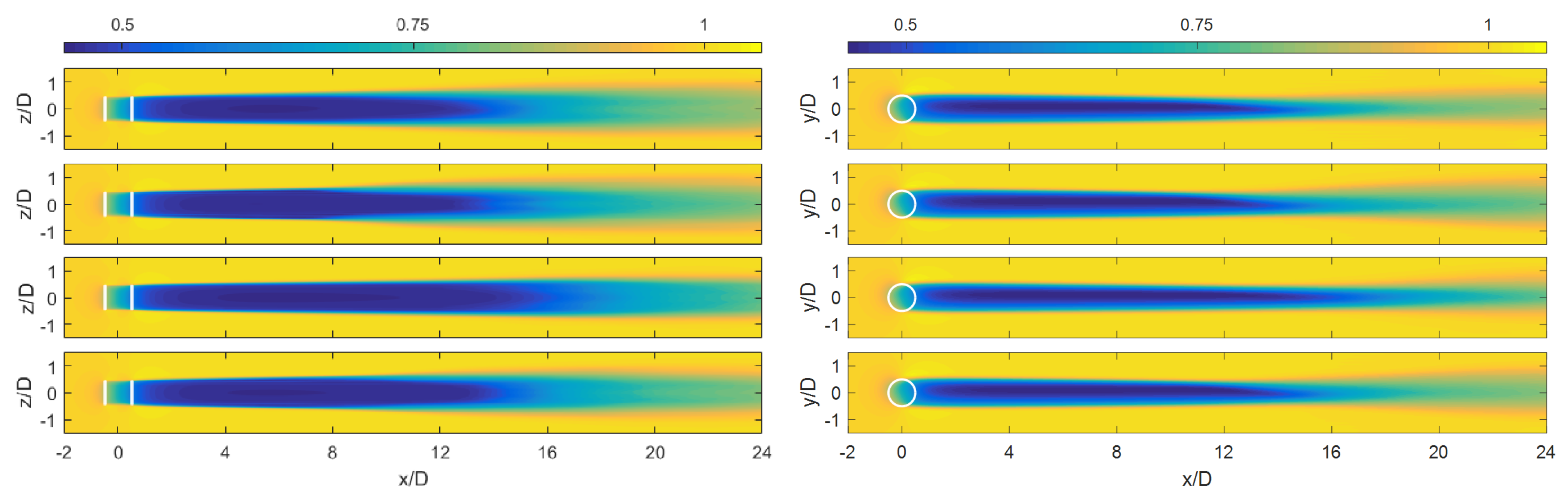
Figure 4.
Vertical (left) and lateral (right) profiles of the normalized mean streamwise velocities () through the turbine equator at downwind of the turbine for different SGS models.
Figure 4.
Vertical (left) and lateral (right) profiles of the normalized mean streamwise velocities () through the turbine equator at downwind of the turbine for different SGS models.

Figure 5.
Contours of the normalized streamwise velocity variance () in the central vertical plane (left) and in the central horizontal plane (right) for different SGS models: (from top to the bottom) LSDD model, AMD model, SMAG model with , and SMAG model with .
Figure 5.
Contours of the normalized streamwise velocity variance () in the central vertical plane (left) and in the central horizontal plane (right) for different SGS models: (from top to the bottom) LSDD model, AMD model, SMAG model with , and SMAG model with .

Figure 6.
Vertical (left) and lateral (right) profiles of the normalized streamwise velocity variance () through the hub level at downwind of the turbine for different SGS models.
Figure 6.
Vertical (left) and lateral (right) profiles of the normalized streamwise velocity variance () through the hub level at downwind of the turbine for different SGS models.

Figure 7.
Contours of the normalized subgrid-scale (SGS) dissipation rate () in the central vertical plane (left) and in the central horizontal plane (right) for different SGS models: (from top to the bottom) LSDD model, AMD model, SMAG model with , and SMAG model with .
Figure 7.
Contours of the normalized subgrid-scale (SGS) dissipation rate () in the central vertical plane (left) and in the central horizontal plane (right) for different SGS models: (from top to the bottom) LSDD model, AMD model, SMAG model with , and SMAG model with .

Figure 8.
Contours of the normalized turbulent kinetic energy (TKE) () in the central vertical plane (left) and in the central horizontal plane (right) for different SGS models: (from top to the bottom) LSDD model, AMD model, SMAG model with , and SMAG model with .
Figure 8.
Contours of the normalized turbulent kinetic energy (TKE) () in the central vertical plane (left) and in the central horizontal plane (right) for different SGS models: (from top to the bottom) LSDD model, AMD model, SMAG model with , and SMAG model with .
© 2018 by the author. Licensee MDPI, Basel, Switzerland. This article is an open access article distributed under the terms and conditions of the Creative Commons Attribution (CC BY) license (http://creativecommons.org/licenses/by/4.0/).
Share and Cite
MDPI and ACS Style
Abkar, M. Impact of Subgrid-Scale Modeling in Actuator-Line Based Large-Eddy Simulation of Vertical-Axis Wind Turbine Wakes. Atmosphere 2018, 9, 257. https://doi.org/10.3390/atmos9070257
AMA Style
Abkar M. Impact of Subgrid-Scale Modeling in Actuator-Line Based Large-Eddy Simulation of Vertical-Axis Wind Turbine Wakes. Atmosphere. 2018; 9(7):257. https://doi.org/10.3390/atmos9070257
Chicago/Turabian StyleAbkar, Mahdi. 2018. "Impact of Subgrid-Scale Modeling in Actuator-Line Based Large-Eddy Simulation of Vertical-Axis Wind Turbine Wakes" Atmosphere 9, no. 7: 257. https://doi.org/10.3390/atmos9070257
Note that from the first issue of 2016, this journal uses article numbers instead of page numbers. See further details here.