Multivariate Interpolation of Wind Field Based on Gaussian Process Regression


1
College of Meteorology and Oceanology, National University of Defense Technology, Changsha 410073, China
2
Beijing Applied Meteorology Research Institute, Beijing 100029, China
*
Author to whom correspondence should be addressed.
Atmosphere 2018, 9(5), 194; https://doi.org/10.3390/atmos9050194
Submission received: 5 April 2018
/
Revised: 11 May 2018
/
Accepted: 15 May 2018
/
Published: 17 May 2018
(This article belongs to the Section Meteorology)
Abstract
:The resolution of the products of numerical weather prediction is limited by the resolution of numerical models and computing resources, which can be improved accurately by a well-chosen interpolation algorithm. This paper is intended to improve the accuracy of spatial interpolation towards wind fields. A new composited multi-scale anisotropic kernel function for weather processes using two-dimensional space information is proposed. To fix the underfitting in this kernel caused by unilateral space information, multiple variables (wind direction, air temperature, and atmospheric pressure) are introduced, which generates a multivariate correction model based on the novel kernel function and Gaussian process regression. Focusing on different weather processes, two multivariate correction models are designed. The new models pave a new way to employ multi-scale local information, and extract the anisotropy and structure information. The experiments on 10 m wind fields for the weather processes without cyclones and for the weather processes with cyclones validate the efficiency. The mean RMSE of the multivariate correction model for the weather processes without cyclones is reduced by around 15% for the u wind component compared with that of a simple composited kernel. For the weather processes with cyclones, the mean RMSE of the novel model declines by around 55% compared to that of spline, and by about 95% compared to that of back propagation neural networks.
1. Introduction
The reanalysis and interpretation of products of numerical weather prediction (NWP) is essential in an NWP system, which is of great importance for the improvement in accuracy of prediction systems [1,2,3,4,5]. However, limited by the resolution of numerical models, computing power, and storage capacity, the resolution of such products are not adequate for more accurate inferences [6,7], such as extreme weather processes analyses. A well-defined interpolation algorithm can increase the resolution of these products more accurately.
Conventional surface fitting methods, such as bilinear and spline methods, are only applicable to specific cases [8]. They are deterministic without taking the randomness of natural weather events into account. Interpolations only rely on local information without taking the anisotropy, physical characteristics, spatial dependences, etc. into consideration [9].
To overcome these problems, several interpolation methods based on different models have been proposed: fuzzy inference [10], hybrid models such as artificial neural networks (ANNs) combined with Kalman filters (KFs) [11], ANNs conjuncted with Markov chains [12], kernel machines such as weighted least square support vector machines (WLS-SVMs) [13], Gaussian process regression (GPR) [14,15,16,17], and so forth. Hybrid models and kernel machines are the mainstay of these new approaches.
With appropriate hybrid components, hybrid models are capable of handling both stationary and nonstationary series. The model that is composed of an autoregressive integrated moving average (ARIMA) model and an ANN is more efficient than either an ANN or an ARIMA alone when forecasting wind speed [18]. Moreover, the KF-ANN model [11], the ARIMA-ANN model [19], and the ARIMA-Kalman model [19] all perform well in forecasting nonlinear wind speed. The increasing number of imported algorithms makes the hybrid models become more effective but more difficult to operate, especially in choosing hybrid components and fine tuning.
Compared with hybrid models, kernel machines (such as SVM and GPR) are easier to operate and can give rise to acceptable results. The proper kernel functions play an important role in kernel machines while predicting winds speed [20,21]. Excluding the choice of kernels, tuning skills required by kernel machines are not as difficult as that by hybrid models because of the single model framework. Hence, kernel machines are the more versatile and simpler models compared with hybrid models.
GPR is one of the most popular methods among various kernel machines. Firstly, the Gaussian process (GP) defines a particular distribution for any finite number of samples. The distribution functions, which are called the family of finite dimensional distributions, reasonably describe the randomness of each sample. For localized and instantaneous weather processes, the sampling environment of each sample cannot be identical. Sampling in the same position at different moments or at the same moment in different positions will result in different distributions for each sample. Secondly, owing to the instantaneity of weather processes [22,23], the influence radius and influence intensity of the wind genesis factors are different. By composing kernel functions, GPR is applied to multi-scale inference, which can extract different radii and intensities [24]. Thirdly, most weather processes with cyclones are non-stationary, whereas the kernel trick in GPR, which means mapping the features in low-dimensional space into high-dimensional space, can handle them. In addition, as a nonparametric algorithm with no demand of the professional tuning skills, it guarantees universality and portability.
Most GPR applications are proposed for time series [14,15,16,17] that handle the wind data sampled in one position at multiple moments. They confirm the efficiency of GPR, but they are not appropriate for interpolating the space series of wind fields sampled from different regions at the same time or sampled from the same time but from different regions. The reasons can be listed as follows. First, most methods for time series take time, or the series itself as the explanatory feature [11,18,19], which is one-dimensional. However, the spatial distributions of the wind fields are two-dimensional at least. Substantially, air temperature, atmospheric pressure, and spatial inhomogeneity influence wind genesis [25,26,27]. Furthermore, for each factor, the influencing radius is not the same [22,23]. A single kernel cannot capture this multi-scale information [28]. In addition, the non-stationary of the spatial series of the weather processes with cyclones is more obvious. However, the kernel for interpolating time series is mostly designed for stationary series [24]. Therefore, considering only a one-dimensional interpreting variable and a single scale without handling the anisotropy, and designing interpolation algorithms only for stationary series, models are blind to spatial series of weather processes. This is a challenge when accurately improving the resolution of products released by NWP.
Considering the relationship of the factors of wind genesis [29,30,31], introducing more information may be one way to meet this challenge. The SVM model, which takes wind speed and temperature or wind speed and wind direction as the input features, generates ideal predictions [32,33]. Grover et al. adopted wind direction, space distance, pressure, and temperature to infer long-range spatial dependencies by GPR [34]. All models work but are not applicable for determining weather processes with cyclones, such as typhoons, which are multi-range dependent and instantaneous. SVM could not capture the different distribution of each sample, which is natural in weather processes. Although GPR can fix this problem by importing random processes, Grover’s proposal can only be used to figure out long-range dependencies. Additionally, the single squared exponential kernel in their method is too smooth for weather processes. To handle multi-range dependencies of the weather processes with cyclones, a multi-scale kernel is required, and more features are needed to correct the underfitting parameters trained by the unilateral spatial information.
Taking all of the above into account, a two-dimensional multi-scale anisotropic kernel function based on GPR is proposed. Taking space coordinates (longitude and latitude) as explanatory variables, the kernel is designed to capture detailed features. Despite the one-sided spatial information, the first principle feature is also introduced as the correction feature to help correct the hyperparameters of the multi-scale anisotropic kernel function. It is generated from air temperature, air pressure and wind direction by principle component analysis (PCA). Different models are specified for weather processes without cyclones and weather processes with cyclones.
The rest of the paper is organized as follows. The basis of the GPR model and the kernel functions associated with weather processes are described in Section 2. Section 3 provides details about the multi-scale anisotropic kernel function for weather processes and the multivariate correction models for spatial interpolation based on GPR. The numerical experiment in Section 4 shows the efficiency of the new models. The dataset used here is ERA Interim [35], a 10 m wind field dataset released by the European Centre for Medium-Range Weather Forecasts (ECMWF). The last section provides conclusions.
2. GPR and Kernel Functions Associated with Weather Processes
2.1. GPR with the Kernel Trick
GPR is a nonparametric algorithm based on a Bayesian framework. The predictions of any finite number have a joint Gaussian distribution [24], which is implied by Equation (3).
Assume there is a training set of n observations, , where denotes the D-dimensional input vector, and y denotes the scalar observed label of . , represent the collection of , y, respectively. The test set of m test input is denoted as . represent the collection of .
Given the training input and the corresponding scalar labels , the optimal interpolation value at any test input in is
The prediction follows a Gaussian distribution
and the joint distribution of and is
where K, , and denote the covariance matrix generated by the kernel function , in which are the input vectors either in the test set or in the training set. Specifically, K denotes the covariance matrix of the training set, denotes the covariance matrix between the training set and the test set, and denotes the covariance matrix of the test set.
Projecting the input vectors in the D-dimensional space into an N-dimensional feature space, GPR is capable of handling nonlinear problem, which is a common characteristic for weather processes. The idea of projecting is also known as kernel trick.
2.2. The Characteristics of Kernel Functions for Weather Processes
A kernel trick is employed in several kernel machines. An abundance of kernels can be chosen.
Different kernels suit different problems. Some are suitable for linear problems, e.g., the linear covariance function; some focus on periodic variation, e.g., the periodic covariance function; some are sensitive to the diversity in different directions, e.g., the Gabor kernel function; and some perform well while describing rough physical process, e.g., the Matérn kernel function.
The most popular kernel is the squared exponential (SE) covariance function, but it is overly smooth for depicting weather processes [24]. The function is expressed as follows:
where , and l is the length-scale hyperparameter.
Fixing the over-smoothness of the SE, the Matérn kernel is suitable for approaching weather processes, especially when , or . The general expression of Matérn kernel is
where and l are the hyperparameters, is a modified Bessel function, and denotes the Gamma function. When , it is simplified as
The Gabor kernel is preferred in image processing for its capability of edge and texture extraction. It is a short-time Fourier transform (STFT) with a Gaussian window function. The variation in wind direction and wind speed between each wind belt is exactly what the Gabor kernel can capture. It is written as
where , denotes the matrix of periodical length-scale hyperparamters, and l denotes the length-scale hyperparamter.
It has been proven that the summation, the product, and the scale of existing kernels are still kernels [24]. Namely,
where denotes a real number. Mapping a kernel to periodic space also gives rise to a kernel that extracts periodic information.
A significant advantage of combining kernel functions is the capability of extracting multi-scale information. By combining the kernels mentioned above according to Equation (8), the new kernel will be capable of extracting multiple pieces of information: periodical information, the diversity in different directions, or rough and localized features. The length-scale hyperparameters of kernels imply the influencing radius of each specific feature.
3. The Multivariate Spatial Interpolation Algorithm
3.1. The Multi-Scale Anisotropic Kernel Function
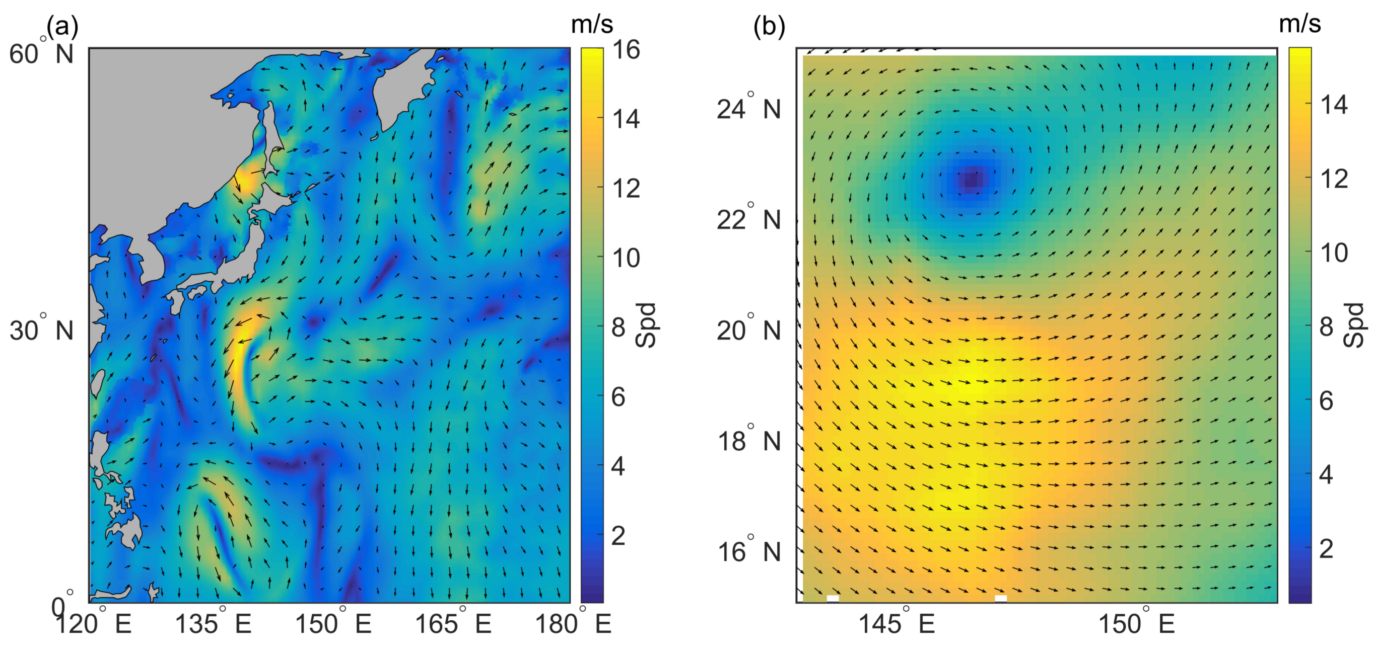
Weather processes are divided into weather processes without cyclones and weather processes with cyclones. Their wind fields are illustrated in Figure 1. Weather processes with cyclones are recognized by the vortexes generated by cyclones. The weather processes without cyclones do not have apparent vortexes.
Considering the analogous distributions of winds between two close positions, the spatial position (longitude and latitude) is taken as the input feature. The closer the positions are, the more similar the winds predicted by the kernel function are.
Moreover, to deal with the anisotropy resulting from the uneven distribution of wind speed and wind direction alongside latitude and longitude, the automatic relevance determination (ARD) pattern is adopted. The anisotropy is implied by in each feature dimension, where denotes the length-scales. The feature with a larger length-scale has a lower influence on the predictions.
For weather processes without cyclones, similar directions of the prevailing winds in each wind belt can be regarded as periodic information. The diversity between wind belts is regarded as the edge, which can be detected by a kernel that is capable of edge extraction. Additionally, real weather processes require a kernel that maintains the roughness rather than filtering it.
The weather processes with cyclones have features similar to those of the weather processes without cyclones. From the typhoon eye to the outside of the vortex, wind fields in the typhoon region change violently but periodically. The vortex texture requires a kernel that is sensitive to the variation in different directions. Additionally, the wind fields of the weather processes with cyclones are rough because of the different changes in wind direction and wind speed alongside each direction.
Considering all of these, the multi-scale anisotropic kernel is proposed for weather processes, which is
where , and represent the Matérn kernel when , the periodical Matérn kernel when , the Gabor kernel, and the noise kernel, respectively. The Matérn kernel describes the roughness of weather processes. For weather processes without cyclones, the periodical Matérn kernel justifies the similarity of each belt. The edge between each wind belt is extracted by the Gabor kernel. For the weather processes with cyclones, the periodical Matérn kernel and Gabor kernel are adopted for the variation in the vortex.
Concretely,
For the Matérn ,
For the periodical Matérn ,
where denotes the Kronecker function.
For the Gabor kernel ,
where is the matrix of periodical length.
Inside,
, , and are unknown here, which are deduced by the logarithm of the marginal likelihood.
3.2. Multivariate Correction Models
Although spacial distributions of wind fields are informative, they are still inadequate to describe the entire fields precisely. Wind genesis is intricate. In addition to the uneven spatial dependence, the influence of Coriolis force, the underlying surface, etc. cannot be ignored [29,30,31,36,37]. Consequently, adopting spatial distribution features only partially determines the natural weather processes. Importing more features can fix that. Thus, the kernel is upgraded to the multivariate correction models and .
Temperature, atmospheric pressure and wind direction are taken as secondary features. However, in view of the potentially redundant information in these features [33], a tradeoff is required. It is proven that the principle components (PCs) corresponding to a large accumulated variance explained ratio of the squared feature vector retains a large possible variance and filters out redundant information in low variability [38].
Assume the secondary features are , the PCs are deduced by
where denotes the covariance matrix of , denotes PCs, and denotes eigenvalues. The accumulated variance explained ratio of top k PCs is
where the eigenvalues correspond to PCs ; and denote the top k eigenvalues and top k PCs, respectively; and n is the total number of eigenvalues or PCs. The reconstructed new feature is
The ratio indicates how much information of is preserved in .
In this study, k is set to one because the of the dataset adopted in Section 4 is at least. However, the choice of k remains open for other datasets. The projected feature of the secondary features is introduced as the new correction feature. This helps correct the multi-scale anisotropic kernel function .
Importing the correction feature, the multivariate correction models are
which is proposed for the series of the meridional region across wind belts without cyclones, and
which is proposed for the non-stationary series of weather processes with cyclones. Among these, denotes the kernel trained by the correction feature . The correction feature contains the auxiliary variability information of the secondary features.
4. A Case Study of Wind Fields 10 m in Height
The dataset of 10 m wind fields used in this study is from the ERA Interim dataset published by the ECMWF. It is subject to global atmospheric reanalysis and has been continuously updated in real time since 1979. The region of the data used in this study ranges from N to N and from E to E. The original resolution of the wind field dataset is . Here, the resolution of the training set is , which is sampled from the original dataset, and the rest are imposed for testing. Concretely, the secondary features are sea surface temperature (SST), mean sea level pressure (MSLP), and wind direction computed from the u wind component and the v wind component.
The efficiency of interpolation is evaluated by the root mean square error (RMSE), which is expressed as
where denotes the i-th predicted u or v wind component, denotes the i-th u or v wind component in the original data, and n denotes the number of the interpolated points. The wind speed of the i-th interpolated point is deduced by
where and denote the u and v wind component either in predictions or in the original data, respectively. The wind speed error of the i-th interpolated point is
where are the i-th u, v wind component from the original data, respectively; and and are the i-th predicted u and v wind components, respectively.
4.1. Weather Processes without Cyclones
The first experiment compares the efficiency of the and models. Because a large region results in a huge covariance matrix that is computationally expensive to invert, the region is divided into subregions firstly and interpolations are then made on each of them. The grid size of each subregion is , which is the number of interpolated points.
To obtain a steady estimation of the unknown hyperparameters mentioned in Section 3.1, each training series is processed 100 times. Two kinds of series are used, one is sampled from different regions at the same time, and the other is sampled from the same region at 20 different moments. After training, the hyperparameters of the series from different regions at the same time are used to interpolate the series at the same moment but from different regions. The hyperparameters of the series at different times in the same region are used to interpolate the series of the same region sampled at other times.
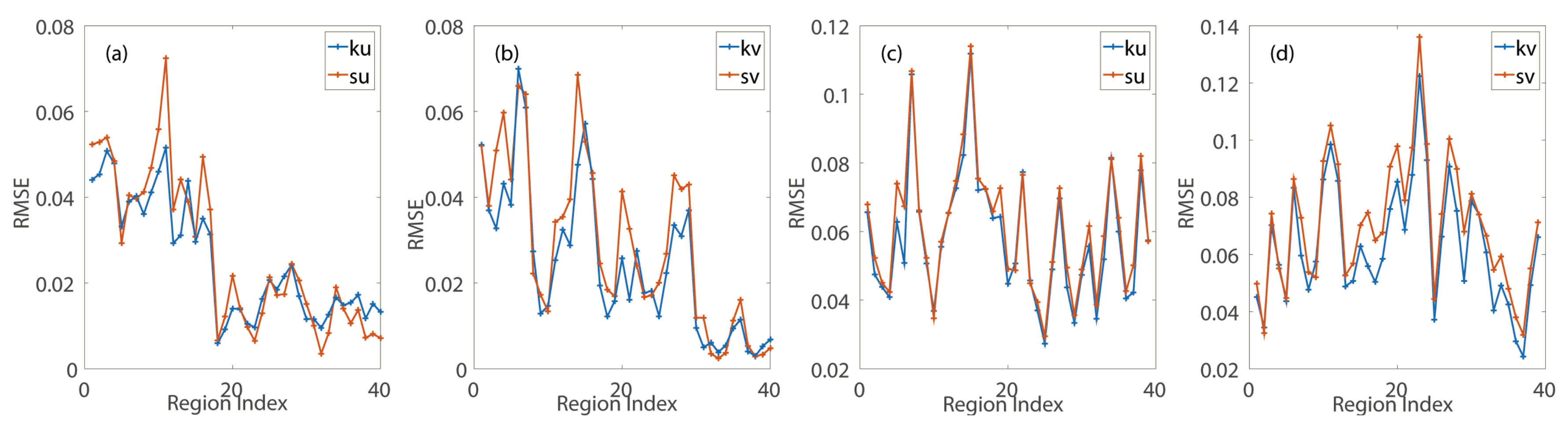
The mean RMSE after interpolating the series sampled from different regions with outperforms the result of the spline method, while the RMSE does not, which is shown in Figure 2a,b. Single multi-scale anisotropic kernel is underfitting while interpolating the space series.
Weather processes without cyclones change seasonally. Interpolating the regions sampled from forty different times (within 10 days of the sampling time in the training set) confirms that what extracts is not contradictory. As shown in Figure 2c,d, in most regions, the RMSE, after interpolating the series sampled from the same region but at different times with , is always smaller than that after interpolation with the spline method.
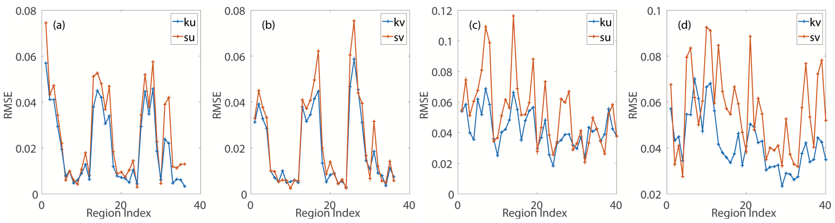
When interpolating the space series sampled from the same time, the mean RMSE of all the interpolated regions with is reduced by at least compared with that of the spline method, which is shown in Figure 3a,b. Additionally, the number of regions increases; the RMSE of these regions is smaller than that after using the spline method. This indicates that has captured the multi-scale local spacial feature. Figure 3c,d shows the results after interpolating the space series sampled from the same region at different times. The mean RMSE of Figure 3c,d declines by for the u wind component and by for the v wind component compared with that of the spline method.
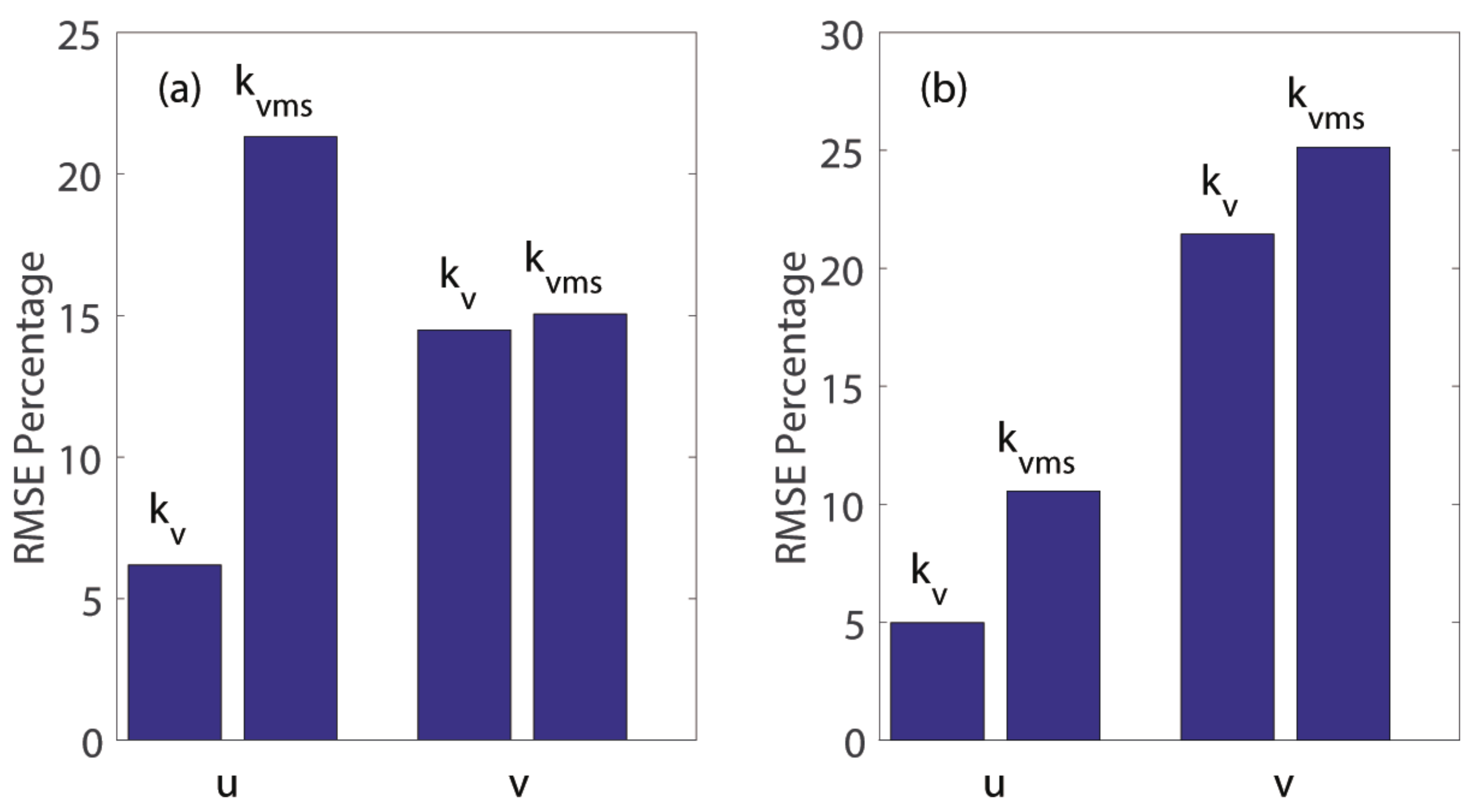
In Figure 4, the promotion of the method, compared with the spline method, outperforms that of the method, which implies that the correction model fixes the one-sided feature trained by single space information.
4.2. Weather Processes with Cylcones
Typhoons Fengshen, Kalmaegi, Fung-wong and Kammuri in 2014 are selected as examples of weather processes with cyclones. Their tracks are shown in Figure 5. Using kernel , 26 regions of Fung-wong that are sampled from 26 different times are trained. The grid size of each region is , which is the number of interpolated points. After training, the hyperparameters are used to interpolate the other typhoon regions sampled from Fengshen, Kalmaegi, and Kammuri.
Except for the baseline spline, the other baseline for comparison is a back propagation (BP) neural networks, which is composited of several fully connected layers. In this study, the entire work can be regarded as a nonlinear regression function. The BP framework used here is shown in Figure 6. All layers, except the output layers, are activated by ReLu activation functions. The output layer is activated by linear activation functions.
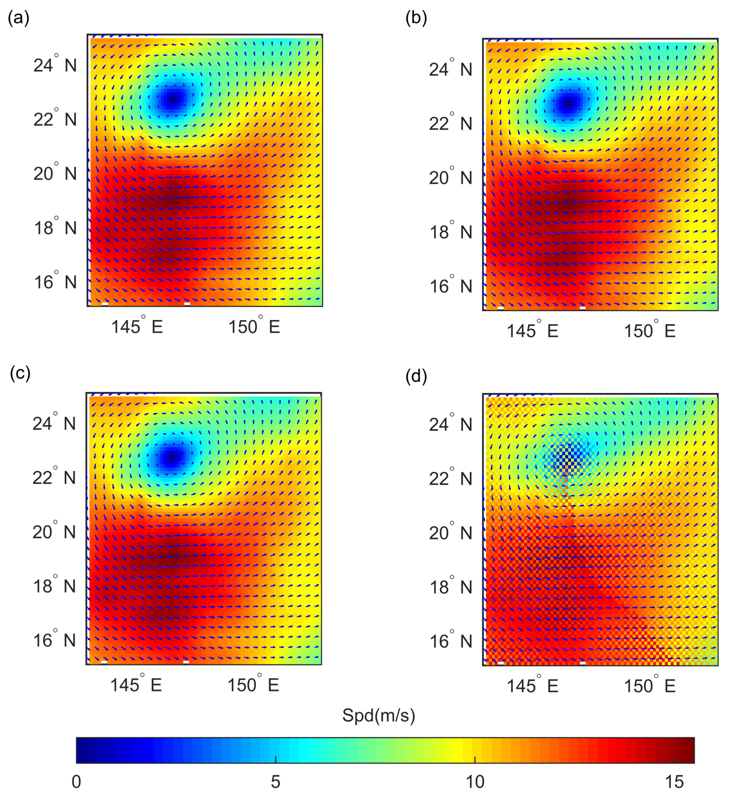
Figure 7 shows the interpolated wind speed and the wind vector field of typhoon Kamurri at 0000 UTC on 26 September 2014. Compared with the reference field shown in Figure 7a, the structural information and scale information are preserved. The field interpolated by BP exhibits an obvious sawtooth phenomenon at the interpolation position. BP adopts wind direction, SST, longitude, and latitude to fit wind fields. It is natural that the result is worse than . There are no scale parameters in BP. What is generated by BP is only a picewise linear function that cannot approach the nonlinear features well. The same features employed in BP are also used to train GPR with a simple multi-scale anisotropic kernel , the result is still under-performing compared with the model. This implies that the major interpreting variables (longitude and latitude) make more sense than the other features, while interpolating wind fields. Spline behaves well owing to the fact that it takes a small number of points around the target point to approach. Although the spline method does not take longer-dependencies into consideration, the result is still acceptable because the weather processes with cyclones dramatically change mainly due to the local environment. However, as shown in Figure 8, Figure 9 and Figure 10, the result of the spline method is still over-smooth in some positions.
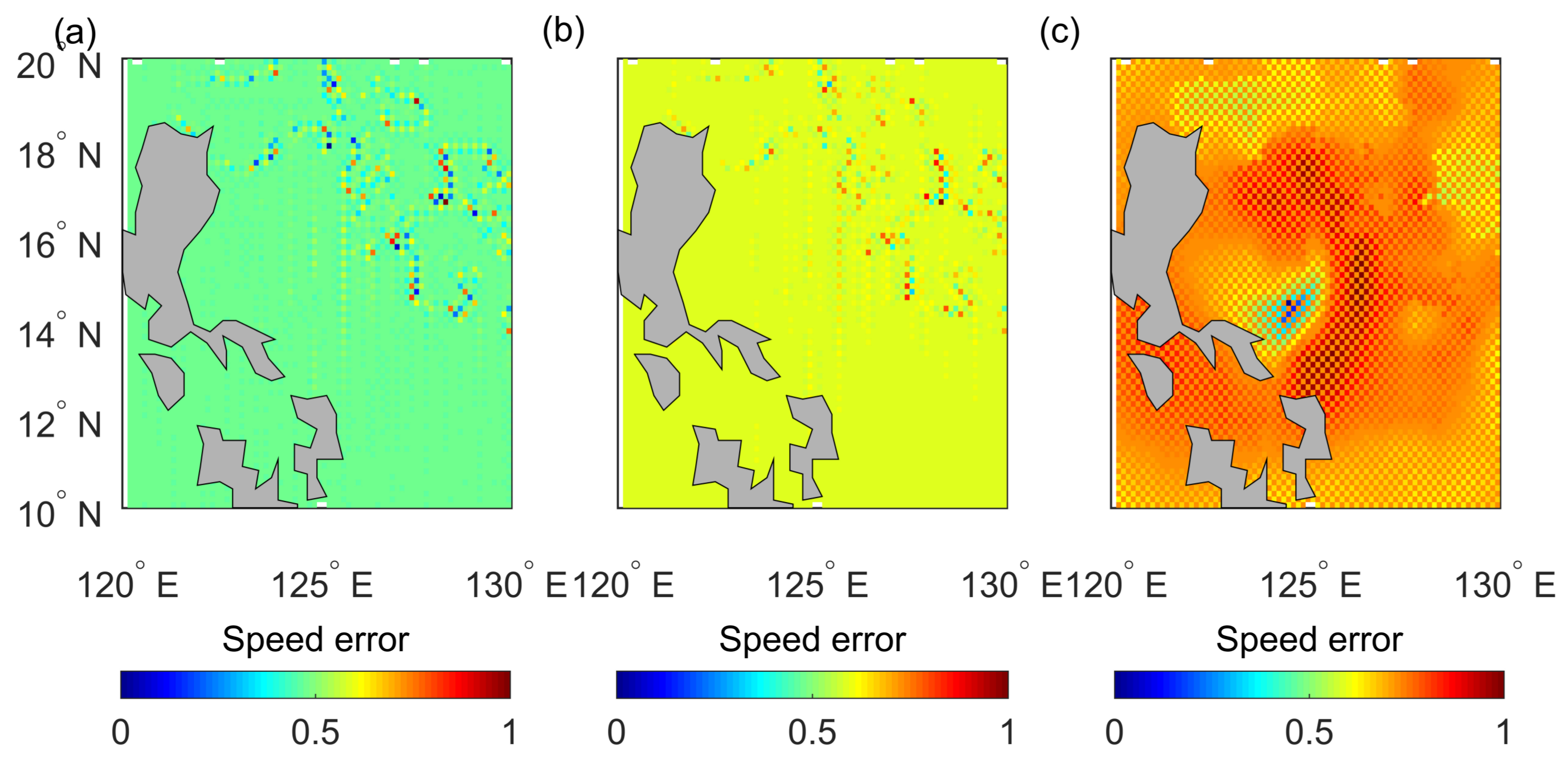
Figure 8, Figure 9 and Figure 10 show the speed error after interpolating. Figure 8 shows the region of Kamurri at 1800 UTC on 28 September, Figure 9 gives the region of Fengshen at 0000 UTC on 8 September, and Figure 10 shows the region of Kalmaegi at 1800 UTC on 13 September. The error bar of the result of in Figure 8 centers around 0.4, which indicates that the mean RMSE of is smaller than that of the spline and BP methods. The speed error of shown in Figure 9 and Figure 10 also validates the improvement. Considering the instantaneous variation of wind speed and wind direction in the vortex, the approach function cannot be too smooth. However, the spline method is over-smooth because it involves two times continuous derivatives. For the Matérn kernel function in the model, the process is mean square continuous (if a sequence of points and a fixed point are assumed, then a process is mean square continuous at if as ), but not mean square differential (if a covariance function is assumed, the mean square derivative in the i-th direction of a process is defined as , where denotes two different input vectors, and denote the vector in the i direction) [24]. This leads to the reasonable roughness that the weather processes require because the smooth function is infinitely derivable in the domain of definition.
The improvement of the mean RMSE in all interpolated regions sampled from Fengshen, Kalmaegi, and Kammuri, after using the hyperparameters trained by Fung-wong, is shown in Table 1.
There is always a tradeoff between accuracy and cost. Although the result of multivariate correction models (either or ) outperforms that of the spline method, the interpolation time of these methods does not. The computing demand of the naive implementation in this experiment is nearly 100 times greater than that of the spline method. The complexity of the spline method is [40], while the main cost of GPR increases as [24]. The inverse of the covariance matrix requires more computing resources. Works focusing on reducing the computing cost of the inverse of the covariance matrix have been published. Fine and Scheinberg proposed the low-rank incomplete Cholesky factorization, which take if the number of decomposition pivots that are greater than the threshold is k [41]. Bae D.H. et al. optimize the memory distribution in a cloud computing system for a massive matrix and made excellent progress [42]. After optimization and parallelization, this method is expected to be operationalized in quickly processing global data generated by NWP systems.
5. Conclusions
In this study, to improve the resolution of products released by the NWP system, a two-dimensional multi-scale anisotropic kernel for the spatial interpolation of wind fields is proposed. To fix the partial information trained by space information, multivariate correction models, namely the model for weather processes without cyclones and the model for weather processes with cyclones, were designed by importing a correction feature (the first principle component of temperature, pressure, and wind direction generated by PCA). The numerical examples of 10 m wind fields in ERA Interim reanalysis demonstrate improvement. Given correction feature, outperforms the spline and simple models. For weather processes with cyclones, interpolating typhoon regions with generates the best result. The model works well compared with the spline and BP methods.
The interpolation time of the models remains undetermined. To construct models that can quickly improve the resolution of global data released by the NWP system, research will focus on reductions in the computation of this naive experiment. Possible approaches include optimizing the inverse algorithm of the massive matrix, GPR sparse inferences or paralleling. After optimization, these new models can be used in variational data assimilation to improve interpolation operators, and this will lead to more accurate forecasting.
Author Contributions
M.F. designed the interpolation algorithms, carried out the study, and wrote the draft. X.Z., B.D., W.Z. and M.Z. participated in designing experiments and analysis. All authors contributed to the writing of the manuscript.
Acknowledgments
The authors would like to thank the support of the European Centre for Medium-Range Weather Forecasts for providing the ERA Interim reanalysis and the National Natural Science Foundation (41675097).
Conflicts of Interest
The authors declare there are no conflict of interest.
Abbreviations
The following abbreviations are used in this manuscript:
| ANN | Artificial Neural Networks |
| ARIMA | Autoregressive Integrated Moving Average |
| ARD | Automatic relevance determination |
| BP | Back Propagation Neural Networks |
| ECMWF | European Centre for Medium-Range Weather Forecasts |
| GP | Gaussian Process |
| GPR | Gaussian Process Regression |
| KF | Kalman Filter |
| MAE | Mean absolute error |
| MSLP | Mean sea level pressure |
| NWP | Numerical Weather Prediction |
| RMSE | Root mean square error |
| SST | Sea surface temperature |
| SVM | Support vector machine |
| WLS-SVM | Weighted least square support vector machine |
References
- Maini, P.; Kumar, A.; Singh, S.V.; Rathore, L.S. Statistical interpretation of NWP products in India. Meteorol. Appl. 2002, 9, 21–31. [Google Scholar] [CrossRef]
- Buizza, R. The Value of a Variable Resolution Approach to Numerical Weather Prediction. Mon. Weather Rev. 2010, 138, 1026–1042. [Google Scholar] [CrossRef]
- Voyant, C.; Muselli, M.; Paoli, C.; Nivet, M.L. Numerical weather prediction (NWP) and hybrid ARMA/ANN model to predict global radiation. Energy 2012, 39, 341–355. [Google Scholar] [CrossRef]
- Chen, Y.; Chen, N.; Wang, S. Application of MOS Method on Pentad Mean Temperature Prediction in Dynamical Extended Range. J. Appl. Meteorol. Sci. 2011, 22, 86–95. [Google Scholar]
- Karl, T.R.; Wang, W.C.; Schlesinger, M.E.; Knight, R.W.; Portman, D. A Method of Relating General Circulation Model Simulated Climate to the Observed Local Climate. Part I: Seasonal Statistics. J. Clim. 1990, 3, 1053–1079. [Google Scholar] [CrossRef]
- Zhang, J.; Draxl, C.; Hopson, T.; Monache, L.D.; Vanvyve, E.; Hodge, B.M. Comparison of numerical weather prediction based deterministic and probabilistic wind resource assessment methods. Appl. Energy 2015, 156, 528–541. [Google Scholar] [CrossRef]
- Kara, A.B.; Barron, C.N.; Wallcraft, A.J.; Oguz, T.; Casey, K.S. Advantages of fine resolution SSTs for small ocean basins: Evaluation in the Black Sea. J. Geophys. Res. Oceans 2008, 113. [Google Scholar] [CrossRef]
- Şen, Z.; Altunkaynak, A.; Özger, M. Space-time Interpolation by Combining Air Pollution and Meteorologic Variables. Pure Appl. Geophys. 2006, 163, 1435–1451. [Google Scholar] [CrossRef]
- Li, J. A Review of Spatial Interpolation Methods for Environmental Scientists; Record Geoscience Australia: 137; Geoscience Australia: Canberra, Australia, 2008. [Google Scholar]
- Yang, Z.; Liu, Y.; Li, C. Interpolation of missing wind data based on ANFIS. Renew. Energy 2011, 36, 993–998. [Google Scholar] [CrossRef]
- Shukur, O.B.; Lee, M.H. Daily wind speed forecasting through hybrid KF-ANN model based on ARIMA. Renew. Energy 2015, 76, 637–647. [Google Scholar] [CrossRef]
- Kani, S.A.P.; Riahy, G.H. A new ANN-based methodology for very short-term wind speed prediction using Markov chain approach. In Proceedings of the 2008 IEEE Canada Electric Power Conference, Vancouver, BC, Canada, 6–7 October 2008; pp. 1–6. [Google Scholar]
- Wang, Q.J.; Zhang, X.F. Effective wind speed estimation for variable speed wind turbines based on WLS-SVM. Acta Simul. Syst. Sin. 2005, 17, 1590–1593. [Google Scholar]
- Chen, N.; Qian, Z.; Meng, X. Multistep Wind Speed Forecasting Based on Wavelet and Gaussian Processes. Math. Probl. Eng. 2013, 2013, 589–606. [Google Scholar] [CrossRef]
- Zhang, C.; Wei, H.; Zhao, X.; Liu, T.; Zhang, K. A Gaussian process regression based hybrid approach for short-term wind speed prediction. Energy Convers. Manag. 2016, 126, 1084–1092. [Google Scholar] [CrossRef]
- Kou, P.; Gao, F.; Guan, X. Sparse online warped Gaussian process for wind power probabilistic forecasting. Appl. Energy 2013, 108, 410–428. [Google Scholar] [CrossRef]
- Yu, J.; Chen, K.; Mori, J.; Rashid, M.M. A Gaussian mixture copula model based localized Gaussian process regression approach for long-term wind speed prediction. Energy 2013, 61, 673–686. [Google Scholar] [CrossRef]
- Cadenas, E.; Rivera, W. Wind speed forecasting in three different regions of Mexico, using a hybrid ARIMA–ANN model. Renew. Energy 2010, 35, 2732–2738. [Google Scholar] [CrossRef]
- Liu, H.; Tian, H.Q.; Li, Y.F. Comparison of two new ARIMA-ANN and ARIMA-Kalman hybrid methods for wind speed prediction. Appl. Energy 2012, 98, 415–424. [Google Scholar] [CrossRef]
- Devi, M.R.; Sridevi, S.; Devi, M.R.; Sridevi, S.; Devi, M.R.; Sridevi, S. Short-term wind power forecasting and predominant wind direction using SVM kernel function. Int. J. Civ. Eng. Technol. 2017, 8, 256–263. [Google Scholar]
- Ouyang, T.; Zha, X.; Liang, Q.; Yi, X.; Tian, X.; Huang, H. Short-term wind power prediction based on kernel function switching. Electr. Power Autom. Equip. 2016, 9, 012. [Google Scholar]
- Capps, S.B.; Zender, C.S. Observed and CAM3 GCM Sea Surface Wind Speed Distributions: Characterization, Comparison, and Bias Reduction. J. Clim. 2008, 21, 2008. [Google Scholar] [CrossRef]
- Segal, M.; Mitchell, M.J.; Arritt, R.W. Sensitivity of Local Deep Convection Potential over Water Bodies to Sea Surface Temperature and Wind Speed. Mon. Weather Rev. 2009, 122, 2210–2217. [Google Scholar] [CrossRef]
- Rasmussen, C.E.; Williams, C.K.I. Gaussian Processes for Machine Learning; MIT Press: Cambridge, MA, USA, 2006. [Google Scholar]
- Adem, J. Relations among Wind, Temperature, Pressure, and Density, with Particular Reference to Monthly Averages. Mon. Weather Rev. 1967, 95, 531–539. [Google Scholar] [CrossRef]
- Wieringa, J. Roughness-dependent geographical interpolation of surface wind speed averages. Q. J. R. Meteorol. Soc. 1986, 112, 867–889. [Google Scholar] [CrossRef]
- Smeets, C.J.P.P.; Duynkerke, P.G.; Vugts, H.F. Observed Wind Profiles and Turbulence Fluxes over an ice Surface with Changing Surface Roughness. Bound.-Layer Meteorol. 1999, 92, 99–121. [Google Scholar] [CrossRef]
- Liu, W.K.; Chen, Y. Wavelet and multiple scale reproducing kernel methods. Int. J. Numer. Methods Fluids 2010, 21, 901–931. [Google Scholar] [CrossRef]
- Toll, A.P. Pressure-Gradient Force; Ceed Publishing, 2012. [Google Scholar]
- Wallace, J.M.; Mitchell, T.P.; Deser, C. The Influence of Sea-Surface Temperature on Surface Wind in the Eastern Equatorial Pacific: Seasonal and Interannual Variability. J. Clim. 1989, 2, 1492–1499. [Google Scholar] [CrossRef]
- Katsaros, K.B.; Soloviev, A.V.; Weisberg, R.H.; Luther, M.E. Reduced Horizontal Sea Surface Temperature Gradients Under Conditions of Clear Skies and Weak Winds. Bound.-Layer Meteorol. 2005, 116, 175–185. [Google Scholar] [CrossRef]
- Peng, H.W.; Yang, X.F.; Liu, F.R. Short-Term Wind Speed Forecasting of Wind Farm Based on SVM Method. Power Syst. Clean Energy 2009, 25, 7. [Google Scholar]
- Huang, R.; Yu, Z.; Deng, Y.; Zeng, X. Short-term wind speed forecasting based on SVM under different feature vectors. Taiyangneng Xuebao/Acta Energiae Sol. Sin. 2014, 35, 866–871. [Google Scholar]
- Grover, A.; Kapoor, A.; Horvitz, E. A Deep Hybrid Model for Weather Forecasting. In Proceedings of the ACM SIGKDD International Conference on Knowledge Discovery and Data Mining, Sydney, Australia, 10–13 August 2015; pp. 379–386. [Google Scholar]
- Dee, D.P.; Uppala, S.M.; Simmons, A.J.; Berrisford, P.; Poli, P.; Kobayashi, S.; Andrae, U.; Balmaseda, M.A.; Balsamo, G.; Bauer, P. The ERA—Interim reanalysis: configuration and performance of the data assimilation system. Q. J. R. Meteorol. Soc. 2011, 137, 553–597. [Google Scholar] [CrossRef]
- Smith, R.K.; Schmidt, C.W.; Montgomery, M.T. An investigation of rotational influences on tropical-cyclone size and intensity. Q. J. R. Meteorol. Soc. 2011, 137, 1841–1855. [Google Scholar] [CrossRef] [Green Version]
- Smith, R.K.; Montgomery, M.T. The efficiency of diabatic heating and tropical cyclone intensification. Q. J. R. Meteorol. Soc. 2016, 142, 2081–2086. [Google Scholar] [CrossRef]
- Karlpearson, F.R.S. LIII. On lines and planes of closest fit to systems of points in space. Philos. Mag. 1901, 2, 559–572. [Google Scholar]
- Ying, M.; Zhang, W.; Yu, H.; Lu, X.; Feng, J.; Fan, Y.; Zhu, Y.; Chen, D. An overview of the China Meteorological Administration tropical cyclone database. J. Atmos. Ocea. Technol. 2014, 31, 287–301. [Google Scholar] [CrossRef]
- Toraichi, K.; Katagishi, K.; Sekita, I.; Mori, R. Computational complexity of spline interpolation. Int. J. Syst. Sci. 1987, 18, 945–954. [Google Scholar] [CrossRef]
- Fine, S.; Scheinberg, K. Efficient svm training using low-rank kernel representations. J. Mach. Learn. Res. 2002, 2, 243–264. [Google Scholar]
- Bae, D.H.; Bayartsogt, M.; Kim, J.S. An algorithm for solving massive matrix inversion in cloud computing systems. In Proceedings of the 2011 ACM Symposium on Research in Applied Computation, Miami, FL, USA, 2–5 November 2011; pp. 61–66. [Google Scholar]
Figure 1.
The wind fields of: (a) weather processes without cyclones; and (b) weather processes with cyclones. The gray patches are lands.
Figure 1.
The wind fields of: (a) weather processes without cyclones; and (b) weather processes with cyclones. The gray patches are lands.

Figure 2.
The RMSE after interpolating: (a) the u wind component; (b) the v wind component; (c) the u wind component; and (d) the v wind component of the test regions with the and spline methods. The series in (a,b) are sampled from different regions at the same time. The series in (c,d) are sampled from the same region at different times. ku and kv denote the RMSE after interpolating u and v wind components with the model, respectively. su and sv denote the RMSE after interpolating u and v components with the spline method, respectively. Region Index denotes the index of the test regions.

Figure 3.
The RMSE after interpolating: (a) the u wind component; (b) the v wind component; (c) the u wind component; and (d) the v wind component of the test regions with the and spline methods. The series in (a,b) are sampled from different regions at the same time. The series in (c,d) are sampled from the same region at different times. ku and kv denote the RMSE after interpolating u and v wind components with the model, respectively. su and sv denote the RMSE after interpolating u and v components with the spline method, respectively. Region Index denotes the index of the test regions.

Figure 4.
The improvement of mean RMSE in percentage after interpolating: (a) the series sampled from different regions at the same time; and (b) the series sampled from the same region at different times. The baseline for comparison is the spline method. denotes the improvement in RMSE over the model and the spline method, denotes the improvement in RMSE over the model and the spline method. u and v denote the u and v wind components, respectively.

Figure 5.
The tracks of typhoons: (a) Fengshen; (b) Kalmaegi; (c) Fung-wong; and (d) Kammuri [39]. The black numbers annotate hours. The time interval of two neighbors in trajectories is 6 h. The color changes of points in the trajectories denote date changes. The green patches are lands. The first point in the trajectories of Fengshen, Kalmaegi, Fung-wong, and Kammuri are sampled at 1400 UTC on 5 September, 1400 UTC on 17 September, 0200 UTC on 11 September, and 0200 UTC on 24 September, respectively. Different marker sizes in figures are only for convenience. For example, the second point of typhoon Fengshen is sampled at 2000 UTC on 5 September, and the third point is sampled at 0200 UTC on 6 September, and so forth.
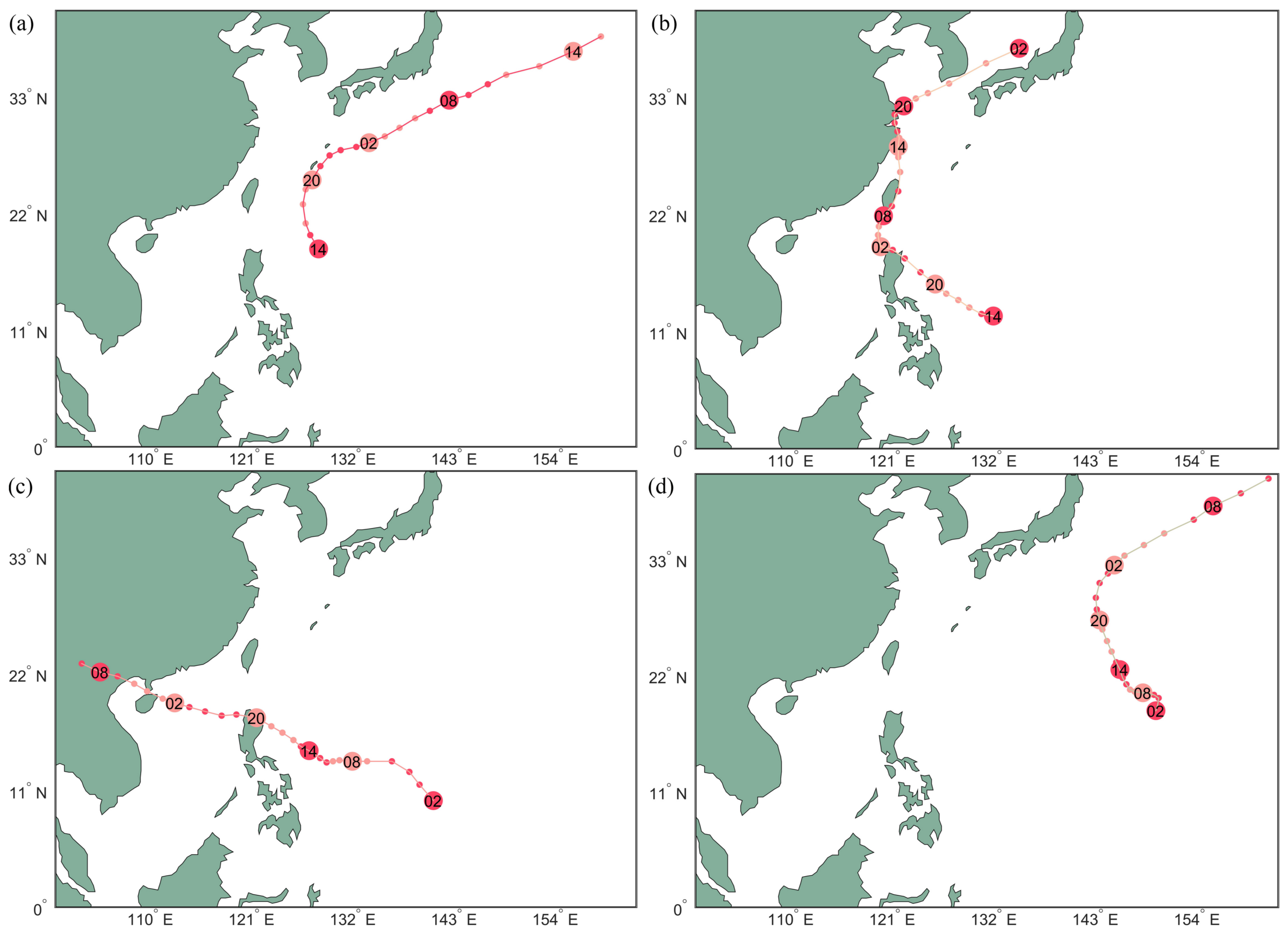
Figure 6.
The BP framework. A dense denotes a layer in BP. The numbers in brackets under input or output denote the dimension of the input data or output data in each layer while running BP. Data flow from left to right.
Figure 6.
The BP framework. A dense denotes a layer in BP. The numbers in brackets under input or output denote the dimension of the input data or output data in each layer while running BP. Data flow from left to right.

Figure 7.
The wind field of typhoon Kamurri after interpolation: (a) reference wind field; (b) ; (c) spline; and (d) BP.
Figure 7.
The wind field of typhoon Kamurri after interpolation: (a) reference wind field; (b) ; (c) spline; and (d) BP.

Figure 8.
The wind speed error of typhoon Kamurri after interpolation: (a) ; (b) spline; and (c) BP.
Figure 8.
The wind speed error of typhoon Kamurri after interpolation: (a) ; (b) spline; and (c) BP.
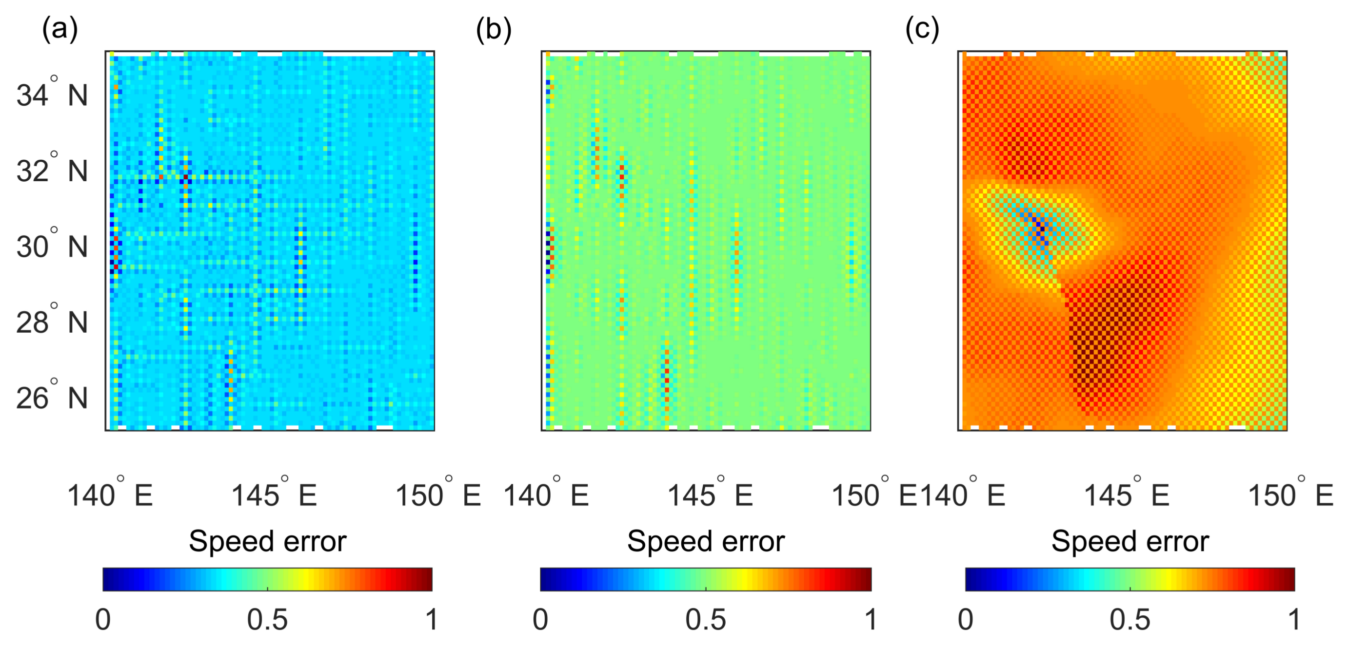
Figure 9.
The wind speed error of typhoon Fengshen after interpolation: (a) ; (b) spline; and (c) BP.
Figure 9.
The wind speed error of typhoon Fengshen after interpolation: (a) ; (b) spline; and (c) BP.
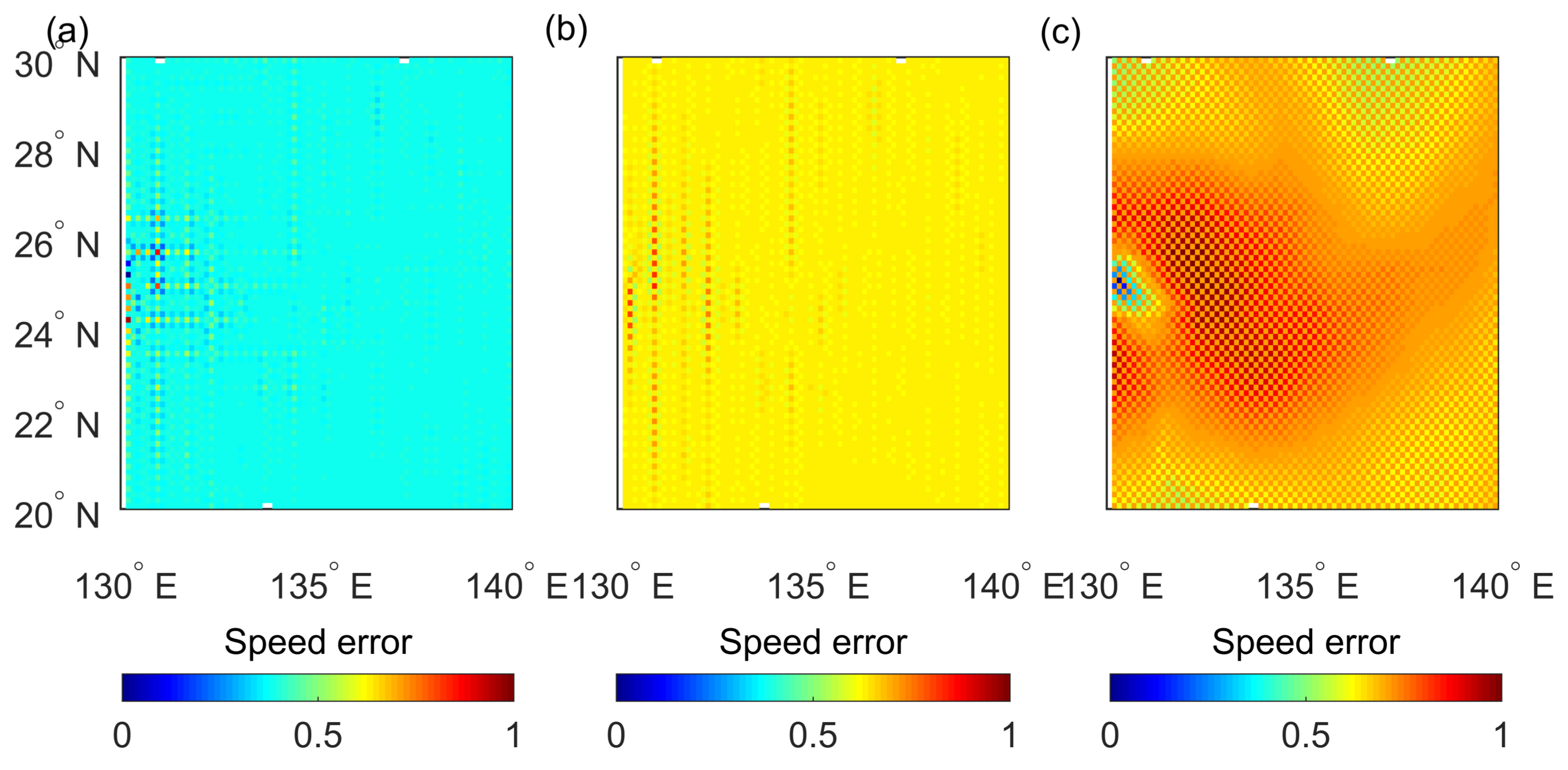
Figure 10.
The wind speed error of typhoon Kalmaegi after interpolation: (a) ; (b) spline; and (c) BP. The gray patches denote lands.
Figure 10.
The wind speed error of typhoon Kalmaegi after interpolation: (a) ; (b) spline; and (c) BP. The gray patches denote lands.

Table 1.
The improvement of RMSE after interpolating typhoon regions with , spline, and BP methods.
| Wind Component | Spline | bp | (%) | (%) | |
|---|---|---|---|---|---|
| u | 0.0492 | 0.1176 | 0.9747 | 58.16 | 94.95 |
| v | 0.0422 | 0.0953 | 0.9822 | 55.72 | 95.71 |
© 2018 by the authors. Licensee MDPI, Basel, Switzerland. This article is an open access article distributed under the terms and conditions of the Creative Commons Attribution (CC BY) license (http://creativecommons.org/licenses/by/4.0/).
Share and Cite
MDPI and ACS Style
Feng, M.; Zhang, W.; Zhu, X.; Duan, B.; Zhu, M.; Xing, D. Multivariate Interpolation of Wind Field Based on Gaussian Process Regression. Atmosphere 2018, 9, 194. https://doi.org/10.3390/atmos9050194
AMA Style
Feng M, Zhang W, Zhu X, Duan B, Zhu M, Xing D. Multivariate Interpolation of Wind Field Based on Gaussian Process Regression. Atmosphere. 2018; 9(5):194. https://doi.org/10.3390/atmos9050194
Chicago/Turabian StyleFeng, Miao, Weimin Zhang, Xiangru Zhu, Boheng Duan, Mengbin Zhu, and De Xing. 2018. "Multivariate Interpolation of Wind Field Based on Gaussian Process Regression" Atmosphere 9, no. 5: 194. https://doi.org/10.3390/atmos9050194
Note that from the first issue of 2016, this journal uses article numbers instead of page numbers. See further details here.