Assessment of the Performance of Three Dynamical Climate Downscaling Methods Using Different Land Surface Information over China

Abstract

This study aims to assess the performance of different dynamical downscaling methods using updated land surface information. Particular attention is given to obtaining high-resolution climate information over China by the combination of an appropriate dynamical downscaling method and updated land surface information. Two group experiments using two land surface datasets are performed, including default Weather Research and Forecasting (WRF) land surface data (OLD) and accurate dynamically accordant MODIS data (NEW). Each group consists of three types of experiments for the summer of 2014, including traditional continuous integration (CT), spectral nudging (SN), and re-initialization (Re) experiments. The Weather Research and Forecasting (WRF) model is used to dynamically downscale ERA-Interim (reanalysis of the European Centre for Medium-Range Weather Forecast, ECMWF) data with a grid spacing of 30 km over China. The simulations are evaluated via comparison with observed conventional meteorological variables, showing that the CT method, which notably overestimates 2 m temperature and underestimates 2 m relative humidity across China, performs the worst; the SN and Re runs outperform the CT method, and the Re shows the smallest RMSE (root means square error). A comparison of observed and simulated precipitation shows that the SN simulation is closest to the observed data, while the CT and Re simulations overestimate precipitation south of the Yangtze River. Compared with the OLD group, the RMSE values of temperature and relative humidity are significantly improved in CT and SN, and there is smaller improved in Re. However, obvious improvements in precipitation are not evident.

1. Introduction

General circulation models (GCMs) are the most commonly used tools for understanding and attributing past climate variations and generating future climate projection. However, their horizontal resolution is often too low to accurately resolve regional or climatic features caused by complex terrain, urban areas, sea-land junctions, and differences in vegetation, land use, and land cover. The downscaling of GCM results or reanalysis data is the main method used to obtain high-resolution regional or local climatic data and establish relationships between global circulation and regional climate [1].

With the development of regional climate models (RCMs) [2,3], dynamical downscaling, which is based on the physical and dynamical frameworks of regional models, has become widely used in downscaling experiments [4,5]. Dynamical downscaling typically begins with a set of coarse-resolution large-scale fields from either GCM or global reanalysis data, which are used to provide the initial (ICs) and lateral meteorological and surface boundary conditions (LBCs) to nested RCMs. The traditional dynamical downscaling approach is to conduct a long-term continuous simulation using the RCMs. The RCMs are intended to add regional detail in response to interactions between regional-scale forcing (e.g., topography, coastlines, land use, land cover, and vegetation) and larger-scale atmospheric circulations [2,6]. Assuming that the large-scale field is correct, the maximization of retained and added values becomes the focus of dynamical downscaling problems. “Value retained” indicates how well an RCMs maintains agreement with the large-scale behavior of the global model forcing data. “Value added” indicates how much additional information the RCMs can provide beyond the highest-resolution global model output or reanalysis data [7,8,9]. During the dynamical downscaling process, errors are introduced in two primary ways. First, error may be introduced through the limited description of RCMs physical processes, including cloud-related processes, cumulus convection schemes, and land surface-atmosphere interactions. Second, error may be caused by coarse-resolution large-scale fields from GCMs outputs or global reanalysis data, which are used as initial conditions and lateral and surface boundary conditions for the RCMs.

RCMs results may drift away from large-scale forcing fields in the traditional dynamical downscaling approach due to the steady accumulation of errors during long continuous model integrations. Using this method, not enough large-scale value is retained by RCMs dynamical downscaling. To address this issue, nudging techniques have been introduced to RCMs that successfully constrain the growth of error in large-scale circulations and simultaneously allow the free development of small-scale circulations [10,11,12,13,14]. Common nudging methods include grid nudging (GN) [10,15] and spectral nudging (SN) [11,16]. GN, in which Newtonian relaxation is used to adjust the model predictions at individual grid points with the same strength, is developed and applied for retrospective meteorological modeling for air quality applications [17,18,19]. SN imposes time-variable large-scale atmospheric states on a regional atmospheric model [11]. SN is scale selective and can be desirable in an RCMs because it relaxes only the longer wavelengths in the simulation toward the driving model fields, which allows small-scale variability from the RCMs to develop. SN also minimizes distortion at the lateral boundaries and eliminates the dependence of the RCMs solution on domain size and position [12,20]. However, the short-wave information provided by RCMs is believed to be more reliable than that provided by GCMs. Therefore, grid nudging has the risk of over-forcing the RCMs at small scales and SN may theoretically outperform GN [18,21,22]. von Storch et al., reported that the SN method could be successful in keeping the simulated states closest to the driving state at large scales, while generating small-scale features [11]. By keeping long waves in the nudging term, Miguez-Macho et al., found that SN can simultaneously help eliminate large-scale precipitation bias and maintain small-scale features [12,23]. Ma et al., performed downscaling experiments over China, showing that SN produces better dynamical downscaling performance for precipitation [24]. In addition, the re-initialization method also has proven effective for the acquisition of regional climatic features [6,25,26,27]. This downscaling method frequently updates the ICs and LBCs and shortens the continuous integration times by running short simulations that are frequently reinitialized. SN and re-initializations have shown excellent downscaling performance in different regions [18,24,27].

In dynamical downscaling, it is critical to obtain as much added value as possible while maximizing the value retained. SN and re-initialization effectively constrain escalating systematic errors during long-term continuous RCMs integrations. Consequently, RCMs can obtain more reliable large-scale circulation features, achieving dynamical downscaling retained value. However, in order to achieve added value, local small-scale features must be embodied in RCMs, which requires RCMs to describe actual atmospheric processes as accurately as possible.

RCMs have significant advantages in the description of local small-scale features because they are coupled with a variety of parameterization processes. Land surface-atmosphere interactions are an important component of the climate system [28,29]. Land surface processes control the exchanges of momentum, heat, and moisture between the land surface and atmosphere, which critically affect the RCMs simulation performance; near-surface meteorological fields and boundary layer processes are extremely sensitive to land surface processes [30,31,32]. An accurate treatment of boundary conditions is a central issue in regional modeling [33,34,35]. Static land surface data are important inputs for regional modeling, as they determine pivotal land surface parameters, such as land use and land cover, vegetation fraction, and leaf area index, reflecting the non-uniformity and complexity of the lower boundary. The accuracy of land surface information affects the determination of land surface processes, which in turn affects the performance of models in simulating regional climate. Enhancing the land surface information accuracy improves the description of land surface processes, more accurately reflecting land surface-atmosphere interactions in RCMs, which in turn delivers more valuable small-scale regional information and achieves added value. However, land surface processes are extremely complicated and affected by various factors. Despite active development, the perfection of land-surface models is a difficult and complex task. As the main two land surface parameters, land use and vegetation reflect the characteristics of different underlying surfaces and affect land parameters in the land surface model [36,37]. Therefore, during the use of different dynamical downscaling methods, updating the dynamically accordant initial land use and vegetation information is a cost-effective and practical way to improve downscaling results in regional models.

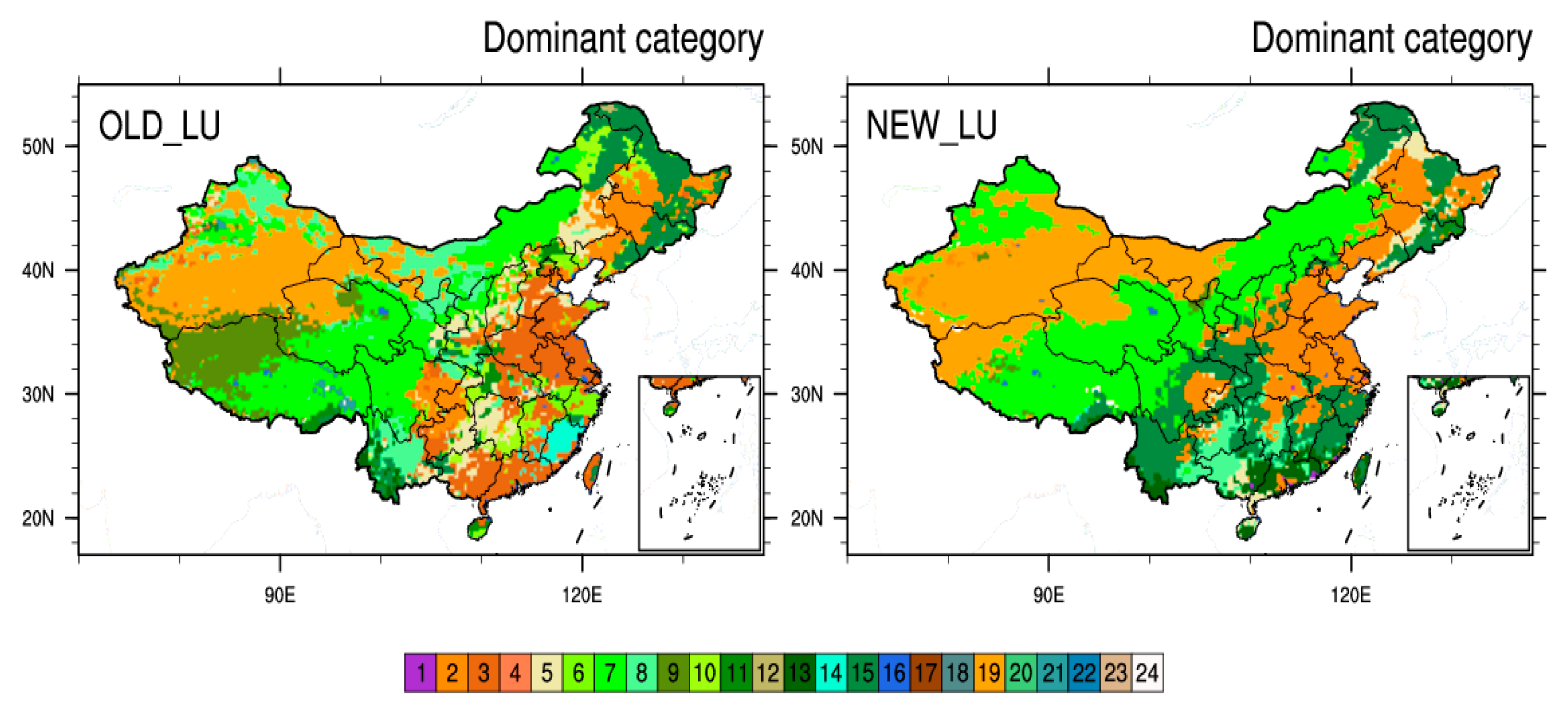
The Weather Research and Forecasting (WRF) model is one of the most widely used regional climate models in dynamical downscaling. It includes two default land use datasets. The first is the Advanced Very High Resolution Radiometer (AVHRR) land use data product developed by the U.S. Geological Survey (USGS) between April 1992 and March 1993, which includes 24 USGS categories [38]. The second is the MODIS land use data product, which was developed at Boston University between January and December 2001 and includes 20 categories developed by the International Geosphere-Biosphere Programme (IGBP) [39]. As mentioned above, the accuracy of these land use data products in China is relatively low [40,41,42]. Wu et al., noted that land use and land cover has changed significantly across China since the beginning of the 21st century [43]. 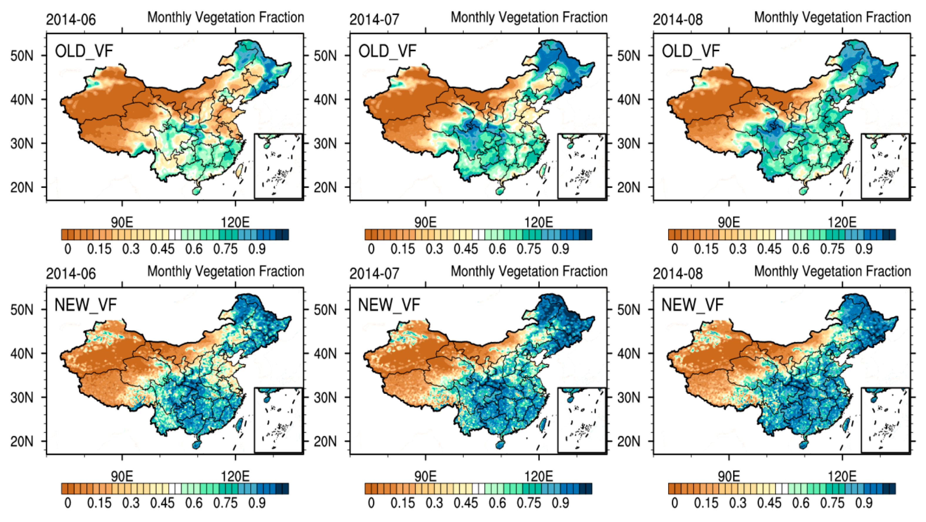The default vegetation fraction of the WRF model is derived from the 5-year AVHRR normalized difference vegetation index (NDVI) climatology, which covers the period from 1985 to 1990 at a resolution of 0.144° [44]. Zhao et al., found that the vegetation fraction over China has changed dramatically in recent years [45]. Li et al., found that compared with the MODIS remote-sensing vegetation fraction, the WRF default vegetation fraction, which was estimated in northeastern China, is becoming gradually less representative [46]. The studies discussed above show that the land surface characteristics given by the default land use and vegetation fraction data of the WRF are no longer particularly representative over China.

A precondition is hypothesized that both SN and re-initialization methods allow the development of small-scale regional information while maintaining large-scale circulation information, and that accurate land surface data improves the model description of land surface process and increases the added value of dynamical downscaling. Therefore, an unresolved problem lies in whether updating dynamically accordant land surface information of land use and vegetation fraction improves dynamical downscaling performance in different dynamical downscaling methods. This study aims to assess the performance of different dynamical downscaling methods (traditional long-term integrations, spectral nudging, and re-initialization) using updated land surface information. Particular attention is given to obtaining high-resolution climate information over China by the perfect combination of an appropriate dynamical downscaling method and updated land surface information. Several experiments were performed involving two experimental groups. One group is based on the WRF default USGS land surface data, and the other is based on updated 2014 MODIS remote sensing land surface data, which is consistent with the simulation period. Each group consists of three tests involving the traditional, spectral nudging, and re-initialization methods. The tests, which feature grid spacing of 30 km over China, investigate the performance of different dynamical downscaling methods and the contribution of updating dynamically accordant land surface data to ERA-Interim (reanalysis of the European Centre for Medium-Range Weather Forecast, ECMWF) dataset downscaling using the WRF model.

The following Section 2 describes the land surface dataset, experimental setup, model details, and the observation datasets that are used to validate the downscaling results. Section 3 presents the results from different dynamical downscaling methods using different land surface datasets. A discussion and summary are presented in Section 4.

2. Data and Methods

2.1. Experimental Setup

In order to assess the performance of different dynamical climate downscaling methods and verify whether the updated dynamically accordant land surface data improve downscaling performance, two group experiments are designed. The first, OLD, is based on the default WRF land surface data, which includes USGS land use and the AVHRR vegetation fraction; the second, NEW, is based on MODIS updated land surface data, including The MODIS Land Cover Type product (MCD12Q1) of land use and MODIS/Terra Vegetation Indices Monthly L3 Global 1 km SIN Grid V006 (MOD13A3) of vegetation fraction during the simulation period. Each experimental group consists of three tests, including the traditional continuous integrations approach (CT), spectral nudging (SN), and re-initialization (Re) methods. Experimental details are provided in

Table 1. Summary of experimental designs.

Experiment	Method	Land Surface Data
		WRF Default	New MODIS
OLD_CT	Tradition method	Yes	No
OLD_SN	Spectral nudging	Yes	No
OLD_Re	Re-initialization	Yes	No
NEW_CT	Tradition method	No	Yes
NEW_SN	Spectral nudging	No	Yes
NEW_Re	Re-initialization	No	Yes

.

2.2. Model Description

The WRF model is used with the Advanced Research WRF (ARW) dynamic core version 3.7 in this study [47]. The model domain is centered at 35° N and 105° E with 220 × 260 horizontal mass grids points at 30 km spacing (Figure 1); it encompasses all of continental China. The Lambert conformal conic projection is used for the model horizontal coordinates. In the vertical dimension, 38 terrain-following eta levels are used from the surface to 10 hPa. Initial and boundary conditions for the large-scale atmospheric fields, as well as initial soil parameters (soil water, moisture, and temperature) are given by the 0.703° ERA-Interim datasets. The domain lateral boundary is composed of a one-point specified zone and a four-point relaxation zone. The main physical options used include the WRF double-moment 6-class (WDM6) microphysical parameterization [48], the community atmosphere model (CAM) longwave and shortwave radiation [49], Yonsei University planetary boundary layer scheme [50], the unified Noah land-surface model [51], Kain-Fritsch cumulus parameterization scheme [52], and community Land Model version 4.5 lake scheme [53,54].

For the traditional continuous integration and SN methods, the model was integrated from 0000 UTC on 22 May to 0000 UTC on 1 September 2014. The initial 10 days are considered to be a spin-up period; the evaluation period spans 1 June to 31 August. When SN is conducted, all waves with wave numbers greater than a preset number are not nudged. In this study, the wave number is set at 5 in both directions (m = n = 5, where m and n represent the wave numbers in zonal and meridional directions, respectively). This preliminary choice is based on two considerations. The first is the scale of the driving field in which the GCM is able to provide reliable information, which is also expected to be captured by RCMs. von Storch et al., determined that scales of about 15° and larger are considered to be reliably analyzed by GCM outputs [11]. The other consideration is the size of the WRF domain. In this study, the WRF domain size is about 6600 × 7800 km in the zonal and meridional directions, respectively. Hence, a wave number of 5 is employed in both directions in order to capture reanalysis data features with scales of 1300–1500 km [18,24].

The Re method simulation was performed using daily re-initialization of the atmosphere as follows. First, the model is initialized at 1200 UTC on 31 May, after which it spins up for 12 h until 0000 UTC and runs until 0000 UTC on 2 June. Then, the model is reinitialized at 1200 UTC on 1 June and spins up again and runs until 0000 UTC on 3 June. After spin-up, the state of the atmosphere is joined with the surface conditions of the previous 24 h simulation. This procedure is repeated throughout the 31 May to 1 September 2014 simulation period. In this manner, the surface conditions remain continuous while the atmosphere is reinitialized every 24 h using ERA-Interim, but with 12 h spin-up period. The individual 24 h simulations are then concatenated in a long climatological time series.

2.3. Land Surface Data

As mentioned above, the accuracy of the MODIS land use data (2001) and 24 categories of USGS land use data (1992–1993) used in the WRF model over China is relatively low [40,41,42]. To explore the effect on downscaling of updated dynamically accordant land surface data, the WRF default USGS land use data are replaced with 2013 MODIS MCD12Q1 land use dataset, which was the latest year available at the time of this analysis. The MODIS land use data product has been evaluated and shown to be highly accurate [39]. The 20 IGBP MODIS land use data categories are converted into the 24 USGS categories, as the IGBP-based classification has limited applicability (and used only in the Noah Land Surface Model).

Table 2. Transformation relationship from 20 categories of land cover data of IGBP to USGS 24 categories, and the proportion of each land category from WRF default data (OLD_LU) and updating MODIS data (NEW_LU) in model domain.

Category	Code		Proportion (%)
	USGS	IGBP	OLD_LU	NEW_LU
Urban and built-up land	1	13	0.007	0.063
Dryland Cropland and Pasture	2	12	7.156	10.273
Irrigated Cropland and Pasture	3	-	6.546	0.025
Mixed Dryland/Irrigated Cropland and Pasture	4	-	0.000	0.000
Cropland/Grassland Mosaic	5	14	2.759	3.635
Cropland/Woodland Mosaic	6	-	1.549	0.290
Grassland	7	10	9.203	13.614
Shrubland	8	6/8	6.108	2.960
Mixed Shrubland/Grassland	9	7	1.591	3.021
Savanna	10	9	2.448	0.072
Deciduous Broadleaf Forest	11	4	1.872	0.250
Deciduous Needleleaf Forest	12	3	3.682	3.152
Evergreen Broadleaf	13	2	1.638	3.539
Evergreen Needleleaf	14	1	1.115	0.712
Mixed Forest	15	5	7.596	10.016
Water Bodies	16	17	41.296	41.096
Herbaceous Wetland	17	11	0.033	0.101
Wooden Wetland	18	-	0.192	0.164
Barren or Sparsely Vegetated	19	16	4.289	6.705
Herbaceous Tundra	20	-	0.000	0.000
Wooded Tundra	21	18	0.787	0.145
Mixed Tundra	22	19	0.019	0.000
Bare Ground Tundra	23	20	0.000	0.000
Snow or Ice	24	15	0.115	0.170

The bold font represents that the NEW_LU data proportion is more than the OLD_LU data in that category. A dash means that the category does not exist in IGBP.

maps these relationships. In Figure 2, the spatial distribution of the 24 default WRF USGS land use categories (Figure 2, OLD_LU) and the updated MODIS products (Figure 2, NEW_LU) in the simulation period are shown at the model resolution. The major land use features of OLD_LU and NEW_LU are similar, but there are numerous regional differences. For example, in northwestern Tibet Plateau, OLD_LU is comprised largely of mixed shrubland/grassland (category 9), which NEW_LU indicates as barren or sparely vegetated (category 19). This is consistent with the results of Liang et al. [55] and Zhang et al. [56]. The cropland/grassland mosaic (category 5) changed to shrubland (category 8) mixed forest (category 15) in the Guizhou and Hunan province (Figure 1). The cropland and pasture (categories 2/3) in northern Guizhou and cropland/woodland mosaic (category 6) in eastern Jiangxi change to shrubland (category 8) and mixed forest (category 15), which is consistent with recent policies calling for the return of farmland to forest in China. The urban and built-up land (category 1) are almost non-existent in OLD_LU, which is not consistent with the current situation. There are, however, urban and built-up land (category 1) in metropolitan areas such as Beijing, Shanghai, and Guangzhou in the updated land use data, which arose from rapid recent urbanization. Table 2 shows the overall land classifications across the continent.

The default WRF vegetation fraction is derived from 5-year AVHRR NDVI climatology, which covers the period from 1985 to 1990 at a resolution of 0.144° [44]. The monthly MODIS MOD13A3 data in summer 2014 within the simulation period are used to calculate the vegetation fraction in the study area. These data have been subjected to quality control to remove the effects of clouds and aerosol pollution. The vegetation fraction calculation method is referred that outlined in Li et al. [46], who used a dimidiate pixel model for quantifying the vegetation fraction from the normalized difference vegetation index, which is derived from the remotely sensed red and near-red bands. In the model, the vegetation fraction (VF) is calculated via the formula:

$${\mathrm{VF}}_{\mathrm{i}}=\frac{{\mathrm{NDVI}}_{\mathrm{i}}-{\mathrm{NDVI}}_{\mathrm{s}}}{{\mathrm{NDVI}}_{\mathrm{v}}-{\mathrm{NDVI}}_{\mathrm{s}}}$$

(1)

where i represents one pixel and NDVI_S and NDVI_V represent the pure pixel NDVI values of barren soil and vegetation, respectively. In the actual calculation, because most of the pixels are mixed pixels, which represent a variety of vegetation types, the calculated vegetation fraction represents the total effect of multiple vegetation types. Therefore, the values of NDVI_S and NDVI_V affect the accuracy of the vegetation fraction. The NDVI_S and NDVI_V values were preset according to Zeng et al. [57] and Miller et al. [58]. Figure 3 shows the distribution of the default WRF (Figure 3 OLD_VF) and updated dynamically accordant vegetation fraction values (Figure 3, NEW_VF) at the model resolution. The vegetation fraction estimated by the MODIS product is higher than that in the WRF default data, especially in southern and northeastern China. These are consistent with the actual land use changes and in agreement with the results of Zhang et al. [56] and Li et al. [46]. The proportions of OLD_VF and NEW_VF at different vegetation fraction levels are shown in

Table 3. Proportion of the OLD_VF and NEW_VF at different vegetation fraction levels in summer 2014.

VF-Level	June		July		August
	OLD_VF (%)	NEW_VF (%)	OLD_VF (%)	NEW_VF (%)	OLD_VF (%)	NEW_VF (%)
VF < 0.2	61.215	53.822	59.437	53.717	57.142	53.268
0.2 ≤ VF < 0.4	8.584	11.098	6.365	9.112	7.170	7.862
0.4 ≤ VF < 0.6	11.196	7.054	8.308	6.194	11.098	5.385
0.6 ≤ VF < 0.8	14.677	10.280	16.143	8.490	17.645	9.416
0.8 ≤ VF	4.329	17.747	9.747	22.488	6.946	24.070

The bold font indicates that the NEW_VF proportion is more than OLD_VF.

.

2.4. Evaluation Datasets and Methods

The datasets provided by the Climatic Data Center of the National Meteorological Information Center (NMIC) of the China Meteorological Administration (Available online: http://data.cma.cn) are used to evaluate downscaling performance. A daily precipitation dataset with a spatial grid resolution of 0.5° is used to assess the downscaling of precipitation simulations. A daily temperature gridded dataset (0.5° × 0.5°) and daily climatic dataset are used to assess downscaling results in terms of the mass field. Each experiment was evaluated across China by comparing the simulated results with the observed data mentioned above using spatial distributions of the variables with all times averaged using statistical verification techniques. The statistical verifications are calculated as follows, where M represents the model simulation values, O represents the observed values, and N is the number of spatial cells so that verifications are computed across all grid cells for each day. The mean error (ME), which indicates whether the simulation over- or underestimates the mean magnitude of the observed values, is defined as follows:

$$\mathrm{ME}=\frac{1}{\mathrm{N}}{\displaystyle \sum }_{\mathrm{i}=1}^{\mathrm{N}}\left({\mathrm{M}}_{\mathrm{I}}-{\mathrm{O}}_{\mathrm{i}}\right)$$

(2)

The root means square error (RMSE), which provides an overview of the accuracy of the simulations and the observations, is defined as follows:

$$\mathrm{RMSE}={\left[\frac{1}{\mathrm{N}}{\displaystyle \sum }_{\mathrm{i}=1}^{\mathrm{N}}{\left({\mathrm{M}}_{\mathrm{i}}-{\mathrm{O}}_{\mathrm{i}}\right)}^2\right]}^{1/2}$$

(3)

The correlation coefficient (cc), which shows the strength of the relationship between the simulation and observed values, is defined as follows:

$$\mathrm{cc}=\frac{\left(1/\left(\mathrm{N}-1\right)\right)[{{\displaystyle \sum }}_{\mathrm{i}}^{\mathrm{N}}\left[\left({\mathrm{M}}_{\mathrm{i}}-\overline{\mathrm{M}}\right)\left({\mathrm{O}}_{\mathrm{i}}-\overline{\mathrm{O}}\right)\right]]}{{\left[\left(1/\left(\mathrm{N}-1\right)\right)[{{\displaystyle \sum }}_{\mathrm{i}=1}^{\mathrm{N}}{\left({\mathrm{M}}_{\mathrm{i}}-\overline{\mathrm{M}}\right)}^2]\right]}^{1/2}{\left[\left(1/\left(\mathrm{N}-1\right)\right)[{{\displaystyle \sum }}_{\mathrm{i}=1}^{\mathrm{N}}{\left({\mathrm{O}}_{\mathrm{i}}-\overline{\mathrm{O}}\right)}^2]\right]}^{1/2}}$$

(4)

The mean improvement rate (RATE), which shows the improvement rate between the OLD and NEW groups for different downscaling methods, is based on RMSE and defined as follows; CRMSE is the RMSE of the OLD group for a given downscaling method, while NRMSE is the RMSE of the NEW group for the same downscaling method.

$$\mathrm{RATE}=\frac{1}{\mathrm{N}}{{\displaystyle \sum }}_{\mathrm{i}=1}^{\mathrm{N}}\left(\frac{{\mathrm{CRMSE}}_{\mathrm{i}}-{\mathrm{NRMSE}}_{\mathrm{i}}}{{\mathrm{CRMSE}}_{\mathrm{i}}}\right)\times 100\%$$

(5)

For the purpose of testing, the true ensemble variances of the OLD group or Re (x) and NEW group or SN (y) are assumed to be equal. Under this assumption, the statistic for the null hypothesis of no difference between the ME, RMSE, and cc values in OLD and NEW group, is given as:

$$t^{\ast }=\frac{\overline{y}-\overline{x}}{s_p\sqrt{\frac{1}{n_y}+\frac{1}{n_x}}}$$

(6)

where the overbar denotes time average, n_x, n_y are the ensemble size corresponding to x and y. The common standard deviation can be estimated by the pooled standard deviation, is given as:

$$s_p=\sqrt{\frac{\left(n_y-1\right)s_y^2+\left(n_x-1\right)s_x^2}{n_y+n_x-2}}$$

(7)

Here, the samples of ME, RMSE and cc are 92-day spatial values in 2014 summer, n_x = n_y = 92, under the null hypothesis of equal means of ME, RMSE and cc from two groups, t* follows the Student’s distribution with f = n_x + n_y − 2 degrees of freedom (f = 182).

3. Results

This section describes the use of observational data to evaluate the downscaling performance of each dynamical downscaling method. The daily mean conventional meteorological elements near the surface include 2 m temperature, 2 m relative humidity, and daily precipitation. The downscaling results of different methods are compared using the default and updated dynamically accordant land surface data. The role of land surface data in the process of downscaling is further explored by analyzing changes in surface heat flux.

3.1. Conventional Meteorological Elements Near the Surface

3.1.1. Temperature

Figure 4 shows the distribution of bias with all times averaged between the simulated and observed daily mean 2 m temperatures during summer 2014 in different experiments. The main factor affecting the spatial distribution of temperature is topography. Due to the influence of the variable terrain in the Tibet Plateau (TP), there are visual features that the spatial distribution of daily temperature bias corresponding variable terrain. The TP temperature simulation shows negative bias in each experiment, as compared to the positive bias seen in other regions.

The CT downscaling method shows the worst downscaling performance. As shown in Figure 4 (OLD_CT and NEW_CT), there are large positive deviations in regions separate from the TP and the RMSE (value averaged over all days; OLD_CT /NEW_CT) is 4.327/4.168 K (

Table 4. The daily spatial ME, RMSE, cc, and RATE of temperature at 2 m for averaged over days in the summer of 2014.

T2		OLD_CT	NEW_CT	OLD_SN	NEW_SN	OLD_Re	NEW_Re
	ME (K)	1.908	1.562	0.259	−0.249	−0.73	−0.457
	RMSE (K)	4.327	4.168	3.167	3.039	2.78	2.729
	cc	0.841	0.873	0.901	0.901	0.903	0.907
	RATE (%)	0.00	3.68	0.00	4.04	0.00	1.84

The bold font represents better skill in the corresponding method.

). The SN method reduces the positive bias seen in the CT method as shown in Figure 4 (OLD_SN and NEW_SN); the RMSE (OLD_SN/NEW_SN) is 3.167/3.039 K. The Re method also reduces the positive bias in study domain apart from the TP, as shown in Figure 4 (OLD_Re and NEW_Re), the RMSE (OLD_Re/NEW_Re) is 2.780/2.729. With decreases in their positive bias, the SN and Re simulations introduce negative bias in the TP. A comparison of the first (OLD) and second (NEW) rows indicates that positive bias that located in east China is reduced in all downscaling methods using updated land surface information (Figure 4; CT/SN/Re). The t-tests (Figure 4; CT_t/SN_t/Re_t) show that there are statistically significant differences in temperature simulations between NEW and OLD at 90% level or higher in eastern China. In particular, there is a large bias in the Sichuan province, which is reduced in the SN simulations by using updated land surface information. This phenomenon indicates that the temperature simulation is sensitive to land use and vegetation fraction; therefore, it is necessary to use accurate dynamic initial land surface data.

In order to quantitatively describe the surface temperature downscaling performance in different experiments, the daily time series of the spatial ME, RMSE, and cc were compared. Figure 5 shows the spatially averaged daily variations of 2 m temperature during the summer of 2014 in different experiments. Meanwhile, this section provides the statistical significance of the difference between OLD and NEW group, SN and Re methods. The results show that the Re method has smallest RMSE (Table 4), followed in order by the SN and CT downscaling methods. Figure 5a shows that changes in the ME and CT method simulations overestimate temperature; this positive bias is reduced in the SN method. Updating the land surface information (NEW) reduces the temperature simulation RMSE in CT and SN dynamical downscaling methods (

Table 5. The results of Student’s-t of spatial ME, RMSE and cc for daily 2 m temperature in summer 2014.

T2		t* (tα = 1.653)
		ME	RMSE	cc
NEW vs. OLD	CT	−2.427	−1.745	5.746
	SN	−15.764	−6.628	0.069
	Re	10.036	−3.267	1.596
SN vs. Re	OLD	23.722	24.570	−2.698
	NEW	16.296	14.881	−0.966

tα is the threshold value of t at the significance level of α, and tα is 1.653 when α = 0.1.

). The surface energy balance is also affected by the surface roughness, reflectivity, and emissivity through their effects on turbulence and surface heat flux; the underlying surface condition determines the surface roughness, reflectivity, and emissivity. Because the initial reflectivity is determined by the static land surface data in WRF, changes in land use and vegetation fraction primarily affect emissivity. Updating the land surface information increases the vegetation fraction, such that the emissivity increases and the net radiant energy on the surface is reduced. With the increased surface roughness of the mixed forest, wind speed decreases, turbulence weakens, heat exchange weakens, and the sensible heat flux decreases. The probability density distribution (Figure 6) also confirms this observation.

In the CT method, bias fluctuates widely with time; the SN and Re methods reduce error and effectively suppress these fluctuations. Furthermore, bias is reduced, and the temperature simulation performance is improved in the NEW group. But the benefits of updating land surface information for the SN and Re methods are not as significant as CT.

3.1.2. Relative Humidity

In the relative humidity simulation, the trend of bias is opposite to that of the temperature simulation. Except for the southern TP, a negative relative humidity bias exists across China; the positive humidity in southern TP is in contrast to the negative temperature bias (Figure 7). The CT method produces a large negative bias (of ~20%) in northeastern China, southern Xinjiang, and North China. The SN method effectively reduces the negative bias in the above-mentioned regions to ~10%. The Re method effective reduce the negative bias in most parts of China, reducing the bias to ~6%. The Re method performs the best for relative humidity in China, followed by the SN and CT methods. Compared with the OLD group, the NEW group, which has updated dynamically accordant land surface data, features improvements in humidity for CT and SN, as well as some improvements in Re, but this improvement was not significant. In the CT and SN simulation results, the negative bias is reduced in the northeastern, and Sichuan regions. In the Re results, the simulated relative humidity is close to the observed value except in the southern TP. In conclusion, relative humidity has a close relationship between evaporation and plant evapotranspiration. Evaporation and plant evapotranspiration are extremely sensitive to the vegetation fraction. By updating the land surface information, models reduce bias in CT and SN methods and improve their simulations of relative humidity. Compared with CT and SN, there is only a minor difference in Re between NEW and OLD. The OLD_Re simulation has a relatively small bias, so compared with OLD_CT and OLD_SN, there is less improvement in the OLD_Re.

Statistical tests allow more detailed examination of the downscaling performance of the three methods. Figure 8 shows daily variations in the mean 2 m relative humidity for the summer of 2014 in different experiments. Figure 9 shows the probability density of the daily relative humidity ME for the summer of 2014 in China. A conspicuous negative ME exists in the CT simulation; the ME values are slightly negative in the SN and Re simulations, but to a lesser degree than that in the CT method. Comparing the three methods, the ME is minimized in the Re simulations, in which it is closer to 1. Comparing the OLD and NEW results, the relative humidity of the simulation increases with the increase in vegetation fraction arising from the updated land surface information, ameliorating most of the negative ME values. Figure 8b shows an RMSE time series in which the CT method has the maximum RMSE, with a mean RMSE (OLD_CT) of 24.034% (

Table 6. Same as Table 4, but for 2 m relative humidity.

RH2		OLD_CT	NEW_CT	OLD_SN	NEW_SN	OLD_Re	NEW_Re
	ME (%)	−13.15	−9.148	−8.529	−5.486	−3.355	−1.774
	RMSE (%)	24.034	20.338	19.539	17.282	15.966	15.209
	cc	0.537	0.591	0.613	0.647	0.649	0.666
	RATE (%)	0.00	15.38	0.00	11.55	0.00	4.92

The bold font represents better skill in the corresponding method.

); the SN mean RMSE (ODL_SN) is reduced, at 19.539%. The Re RMSE (OLD_Re) is the smallest, at 15.966%. The introduction of the updated land surface information obviously improves the CT and SN methods (

Table 7. Same as Table 5, but for 2 m relative humidity.

RH2		t* (tα = 1.653)
		ME	RMSE	cc
NEW vs. OLD	CT	4.900	−5.578	2.899
	SN	5.244	−3.990	1.729
	Re	2.713	−1.383	0.832
SN vs. Re	OLD	−8.863	6.212	−1.717
	NEW	−6.409	3.856	−0.951

), which have RATE values (NEW_CT and NEW_SN) of 15.38% and 11.55%, respectively. There is no clear improvement in the Re method, for which the RATE value (NEW_Re) is 4.92%. The cc results echo the ME and RMSE results. In the Re method, the spin-up time is short due to the frequent updating of initial information. Thus, the effect of the land surface information on the climate field is not cumulative, and the land surface information has little effect on the Re method.

3.2. Precipitation

In this section, the spatial distributions and temporal variations of total daily accumulated precipitation (mm/day) are described. Figure 10 shows the observed spatial distributions and temporal variations of diurnally averaged precipitation during the summer of 2014 over China (Figure 10a,b). The daily precipitation presents obvious features, showing abundant precipitation in the south and scarce precipitation in the north. Precipitation is less than 6 mm north of the Yangtze River and 6–10 mm south of the Yangtze River, with individual areas featuring more than 10 mm. Figure 11 compares simulated diurnally averaged precipitation bias from the three methods using OLD and NEW land surface data during the summer of 2014 over China. The mean diurnal characteristics of precipitation are captured well north of the Yellow River, but somewhat overestimated south of the Yellow River. China is located in the Asian monsoon region, and the monsoonal circulation plays an important role in the transport of water vapor. Thus, the distribution of seasonal precipitation is strongly influenced by the Asian monsoon. Precipitation is also significantly affected by the large terrain; seasonal precipitation in China has long challenged meteorologists due to the complexity of the East Asian topography. Of the three methods, the CT and Re methods overestimated precipitation in the eastern TP, Northeast Plain, and Hunan Jiangxi province junction. The Re method clearly overestimated precipitation in the eastern TP, while the CT method clearly overestimated precipitation in the Hunan Jiangxi province junction. However, mean precipitation is realistically simulated by the SN method, which produces only a small positive bias in the southwestern region. The SN provides large-scale flow consistent with the large-scale reanalysis circulation, which prevents the model results from drifting away from the large-scale circulation above the boundary layer and shows advantages for precipitation simulation. The Re method frequently updates the ICs and LBCs with more detailed topography and performs reasonably well in downscaling surface parameters. Updating the land surface information does not adjust the large-scale circulation field, so these updates do not improve precipitation caused by large-scale circulations. The Re simulation runs with a shorter spin-up time, subdivide some parameters, which generally have long memory (such as soil parameters) from a long simulation into shorter ones. This problem should be addressed in the design of optimal re-initialization spin-up times.

Relationships between verification parameters and observations are shown in Figure 12. Figure 13 shows the probability density of the daily accumulated precipitation ME.

Table 8. Same as Table 4, but for daily accumulated precipitation in summer, 2014.

Precip		OLD_CT	NEW_CT	OLD_SN	NEW_SN	OLD_Re	NEW_Re
	ME (mm)	1.832	2.082	1.106	1.428	2.461	2.594
	RMSE (mm)	15.479	15.292	11.04	11.09	11.638	11.65
	cc	0.051	0.091	0.432	0.429	0.118	0.111
	RATE (%)	0.00	1.21	0.00	−1.03	0.00	−0.45

The bold font represents better skill in the corresponding method.

shows a summary of the ME, RMSE, cc, and RATE for daily accumulated precipitation in summer 2014 over China. The CT runs feature the maximum RMSE (OLD_CT/NEW_CT) (Figure 12b, Table 8), while the Re method overestimates precipitation during all of the experiments (Figure 12a). Compared to the CT and Re methods, the SN simulations show minimal RMSE and the highest correlations with observed data (Table 8), and, therefore, outperform the other downscaling methods for daily mean precipitation. This is consistent with the spatial distribution results discussed earlier. In these tests, there is no obvious change between the NEW and OLD groups in the precipitation simulation (Figure 13,

Table 9. Same as Table 5, but for daily accumulated precipitation in summer, 2014.

Precip		t* (tα = 1.653)
		ME	RMSE	cc
NEW vs. OLD	CT	0.803	−0.261	2.522
	SN	1.594	0.137	0.136
	Re	1.070	0.035	0.443
SN vs. Re	OLD	−8.229	−1.610	17.262
	NEW	−6.847	−1.547	16.907

).

3.3. Surface Heat Flux

The land surface energy balance is significantly affected by the land surface initial information, and surface latent heat flux and sensible heat flux are important components of the surface energy balance. Surface energy balance is reflected in changes in mean surface sensible heat flux and latent heat flux. Therefore, these variables can be explored to gain a better understanding of the effect of updating land surface information on the surface energy balance in different downscaling methods. Figure 14 shows three-month (JJA-2014) average sensible heat flux (W m⁻²) from the OLD model simulation and differences with the corresponding NEW model simulations in the three downscaling methods. In the different downscaling methods, the sensible heat flux is similar to the general trend, but differences exist in many areas. In the Xinjiang and northeast China regions, the SN sensible heat flux exhibits a larger order of magnitude, followed in order by the CT and Re methods. South of the Yangtze River, the sensible heat flux magnitudes simulated by the SN and Re methods are similar, and that simulated by the CT method is small. There is a change in the sensible heat flux after updating the land surface information. The sensible heat flux variation trends are similar in the different downscaling methods, but the magnitude variation differs in different regions. For instance, in northeastern China, the land surface information update leads to an increased vegetation fraction and the sensible heat flux is decreased; these changes are most obvious in the CT method (Figure 14, NEW_CT), followed by the SN (Figure 14, NEW_SN) and Re methods (Figure 14, NEW_Re). However, in the northwestern TP, in which the land surface information update changes the land categories from mixed shrubland/grassland (categories 9) to barren or sparsely vegetated (categories 19) areas, the sensible heat flux is increased in the CT and Re methods, with the clearest increases in the CT method. In the northeast part of the Yunnan province, where shrubland (categories 8) are transformed into mixed forest (categories 15), the sensible heat decreases; in the southern Guizhou, where the broadleaf forest (categories 12) changes to shrubland (categories 8), the sensible heat flux increases. In the Sichuan province, a large area of cropland and pasture (categories 3) changes to broadleaf (categories 13), the vegetation fraction is increased, and the sensible heat is reduced.

The trend of latent heat flux is opposite to that of the sensible heat flux (Figure 15). In summer, in the Xinjiang area, which features a large desert, moisture is scarce, and the sensible heat flux is dominant; the latent heat flux is small compared to the sensible flux. The variations in latent heat flux are similar between the three downscaling methods; the vegetation fraction, and thus evapotranspiration, increases over most of China, and these changes are most obvious in the northeastern and Sichuan province. In southern Guizhou, the latent heat flux is reduced due to the conversion of deciduous broadleaf forest (categories 11) to mixed forest (categories 15).

4. Summary and Discussion

The performance of dynamical downscaling is affected by diverse geographical, seasonal, regional climate model, and driven field factors. In this paper, the performance of three dynamical downscaling methods, including the CT, SN, and Re methods, are compared. The effect of updated static land surface information on downscaling performance is also explored for the three dynamical downscaling methods. Two groups of experiments are performed using WRF, one based on the default WRF USGS land use data and AVHRR vegetation fraction data, and the other based on MODIS land use and vegetation fraction data consistent with the selected simulation period. Each group of experiments contains runs using the CT, SN, and Re methods in which dynamical downscaling is performed for ERA-Interim reanalysis data at a resolution of 30 km in the summer of 2014 over China. The downscaling results, which include conventional meteorological elements and precipitation, are evaluated against observation data provided by the NMIC. The mechanisms are examined by which changes in land surface information affect near-surface variables and precipitation in the three dynamical downscaling methods.

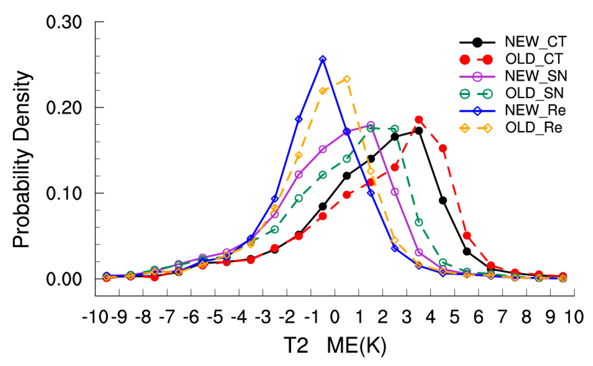
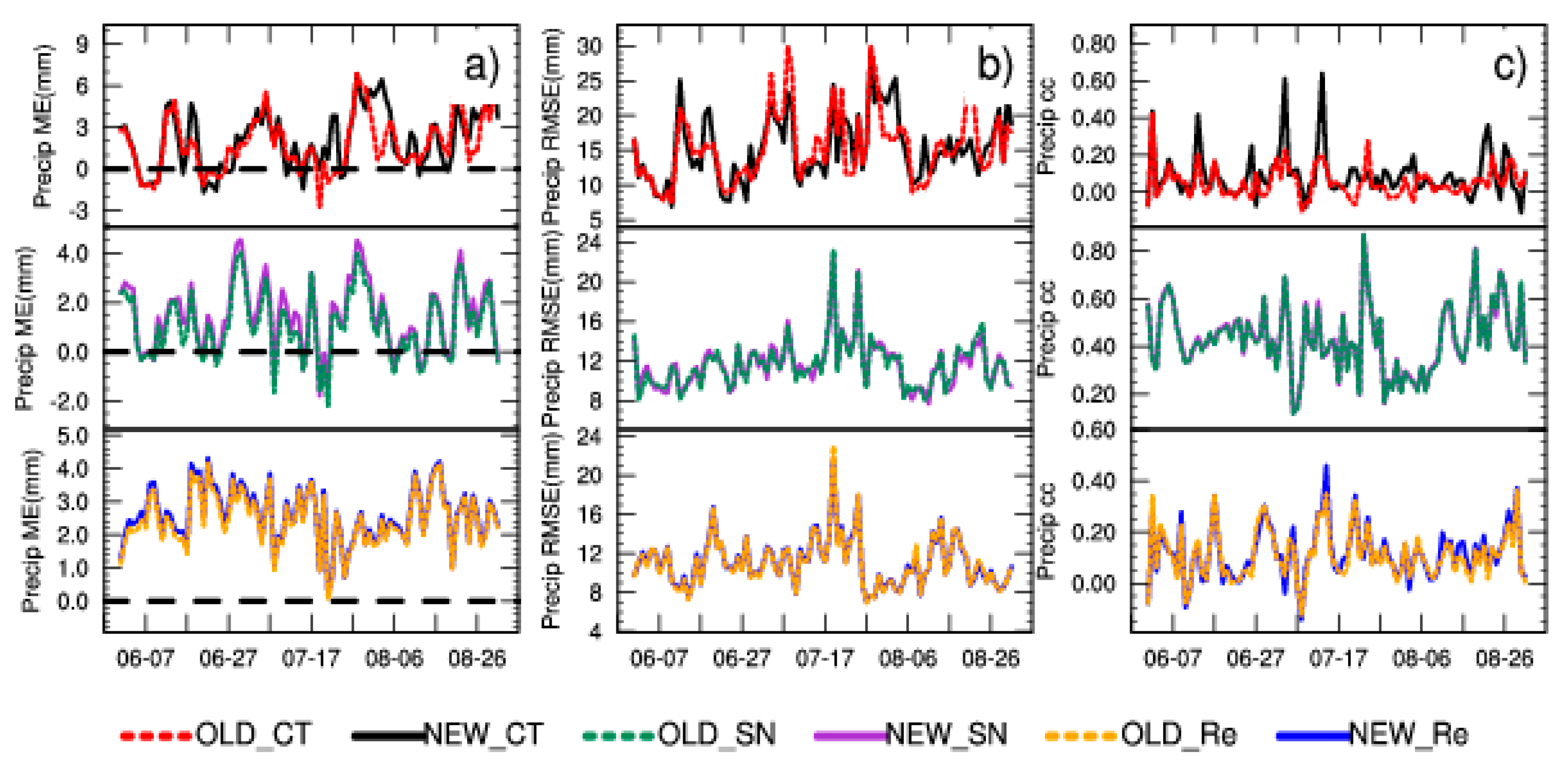
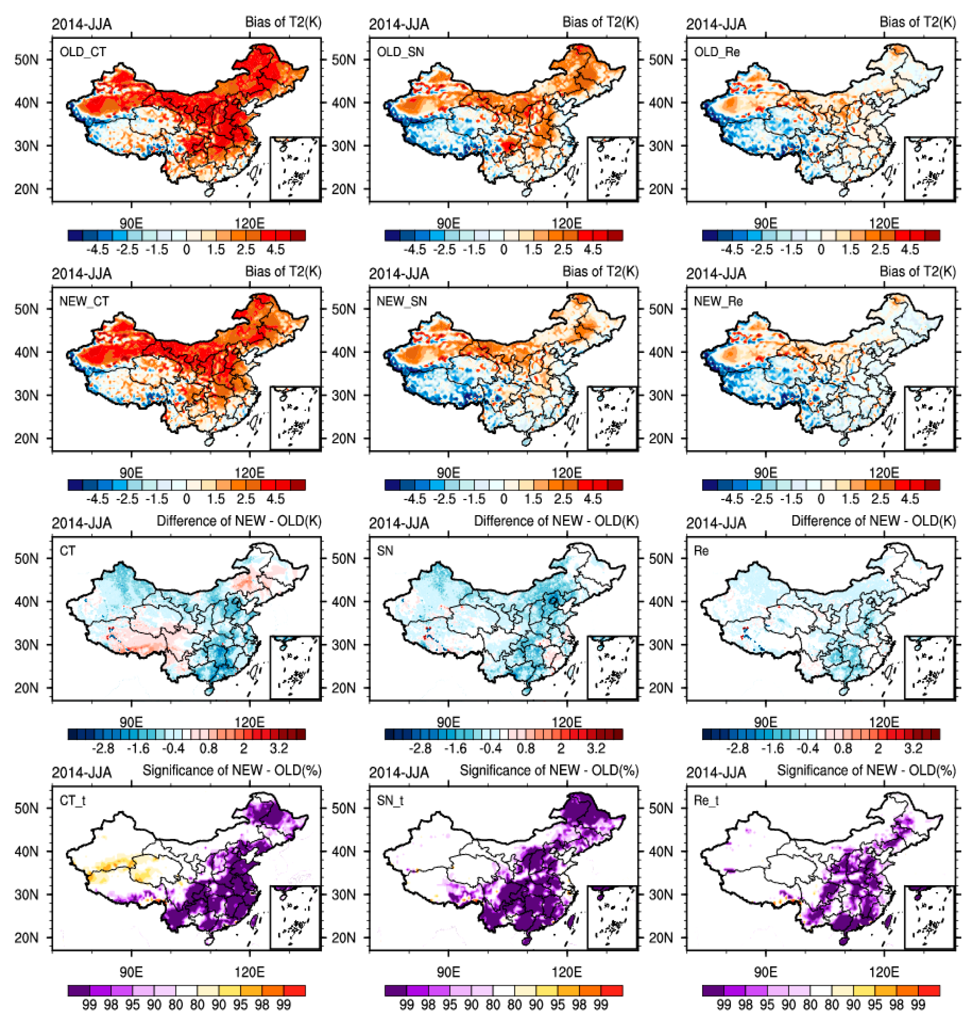
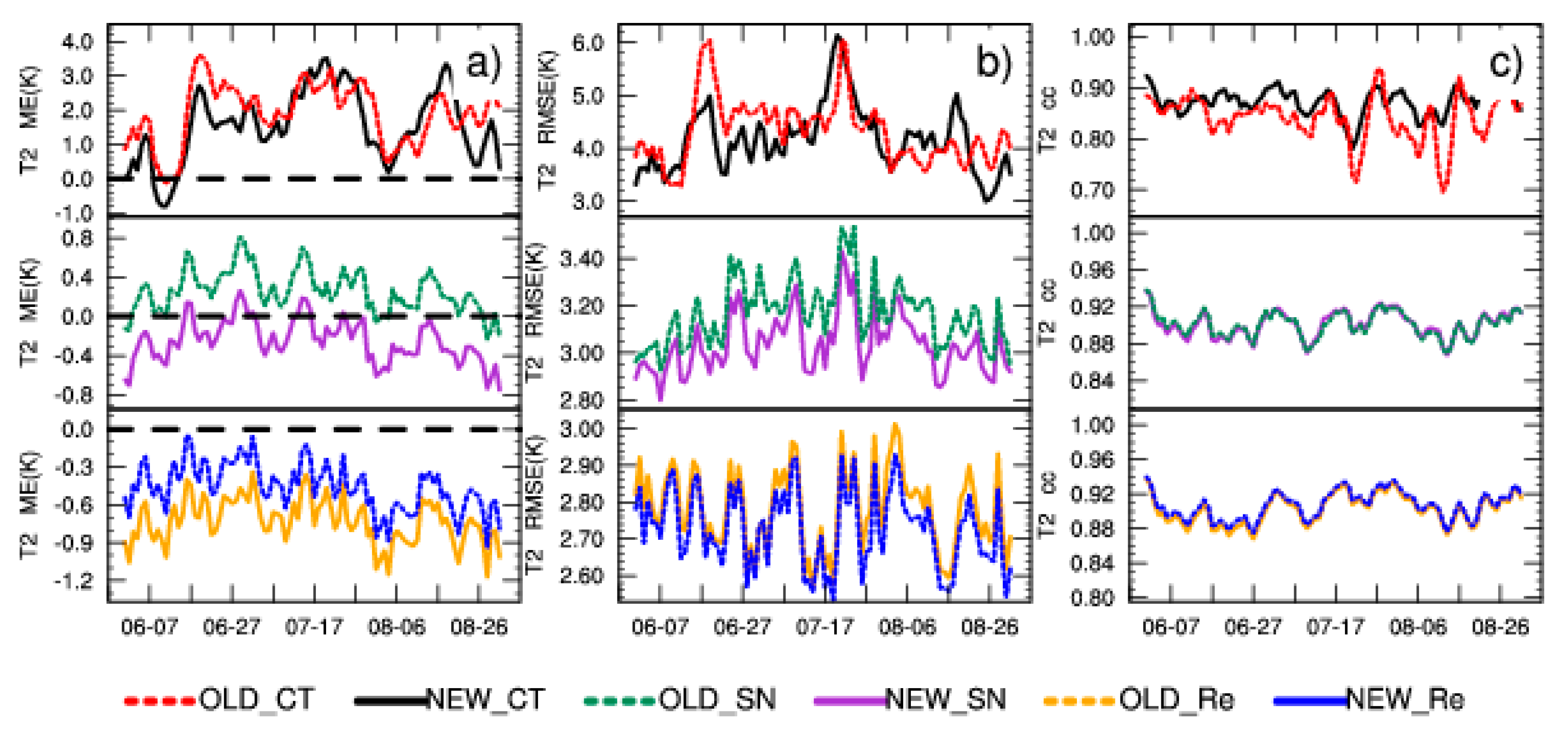
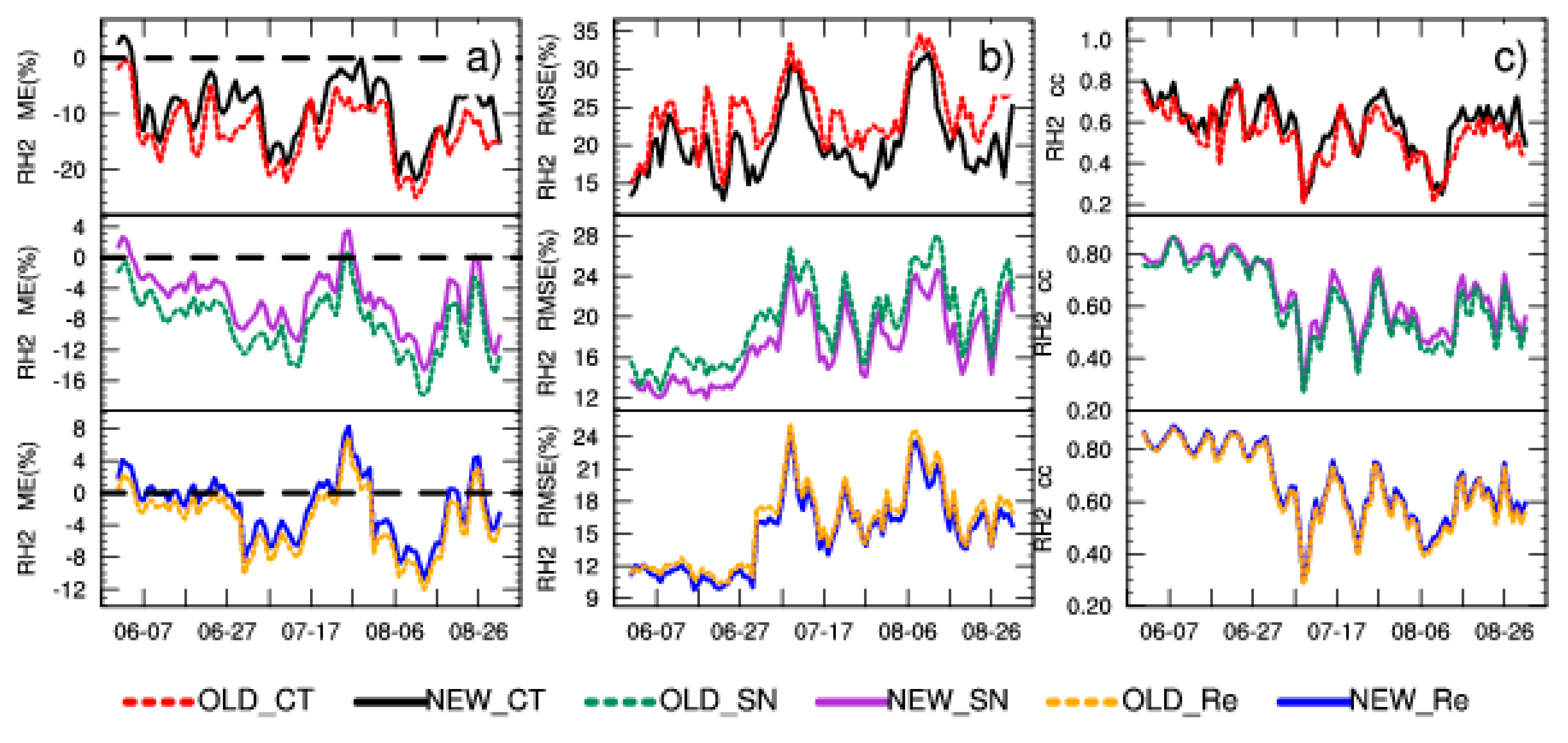
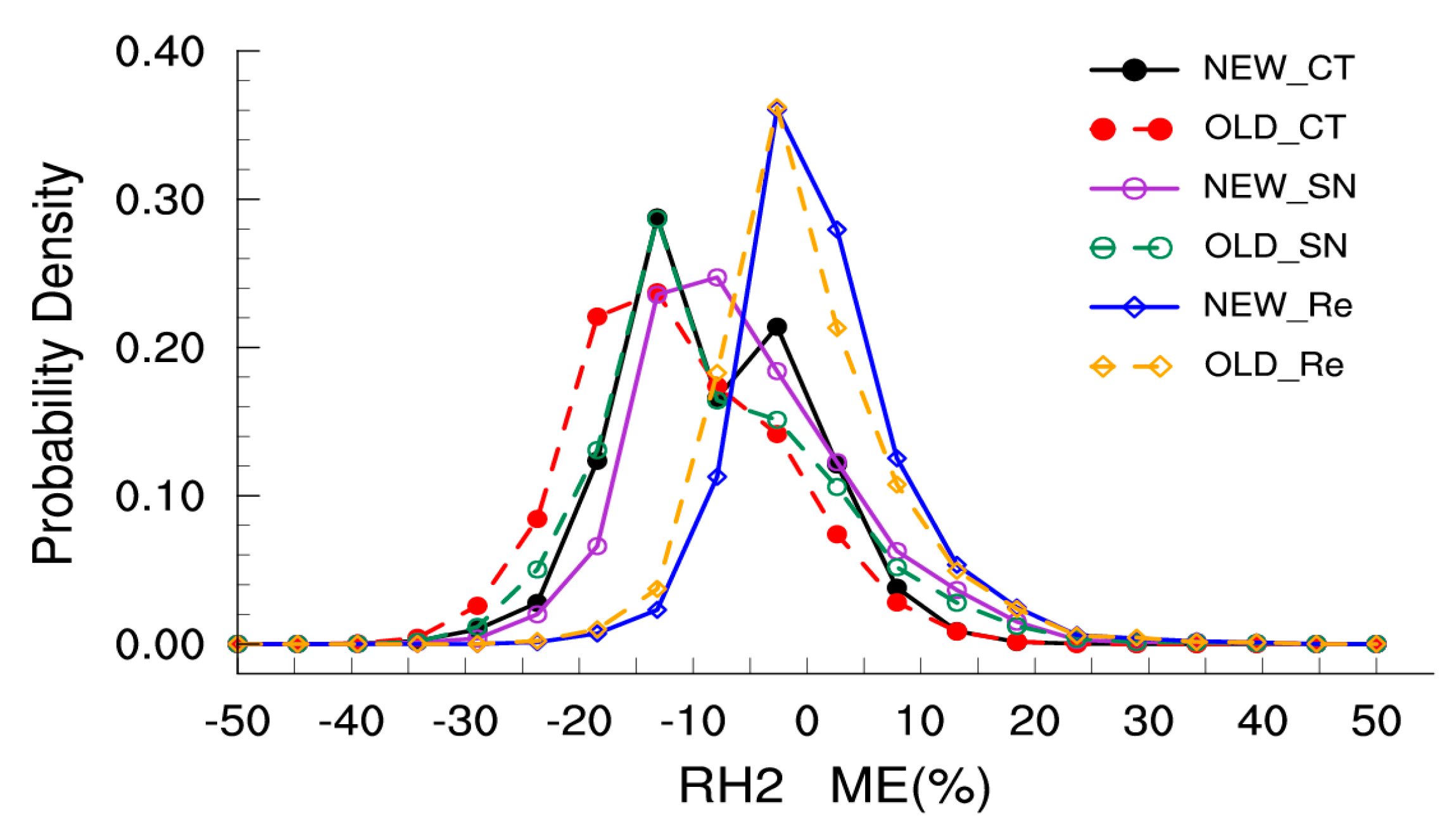
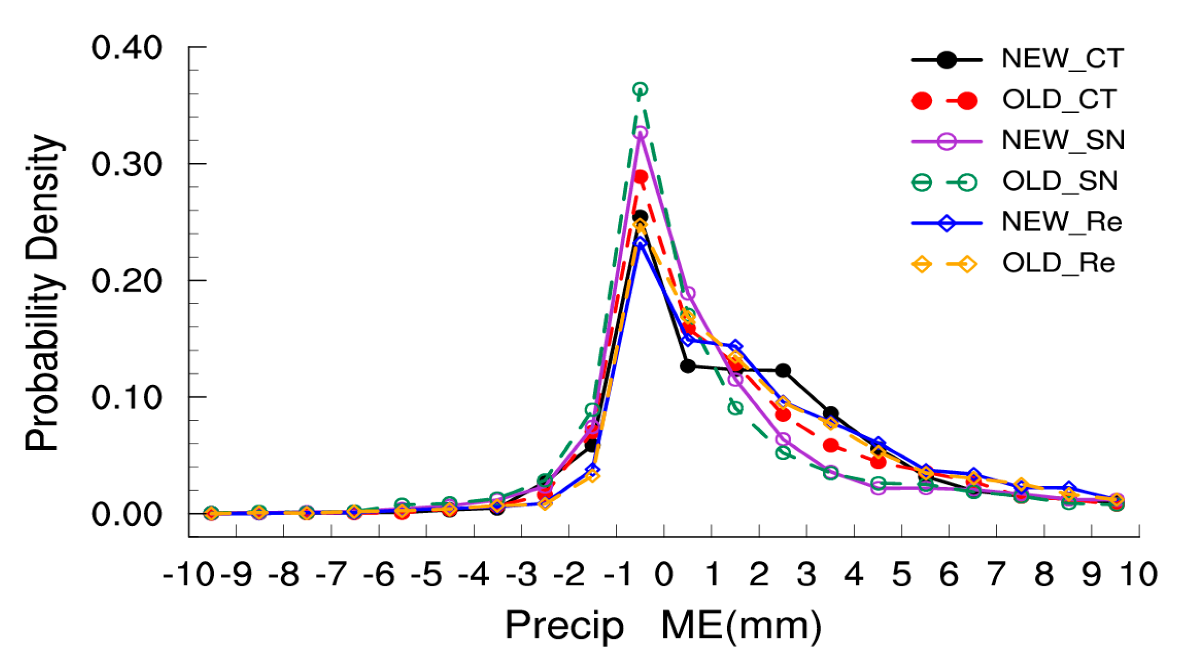
The significant conclusions drawn from the 2 m temperature and relative humidity are as follows. The traditional continuous integration approach (CT) shows the worst performance among the downscaling methods. The model drifts away from the forcing ERA-Interim reanalysis over the course of long integrations, and the simulations seriously overestimate surface temperature and underestimate relative humidity (except in the TP region). The SN downscaling simulations perform better than CT, reduces the temperature overestimation and relative humidity underestimation. The Re method has smallest RMSE in 2 m temperature and 2 m relative humidity simulations. 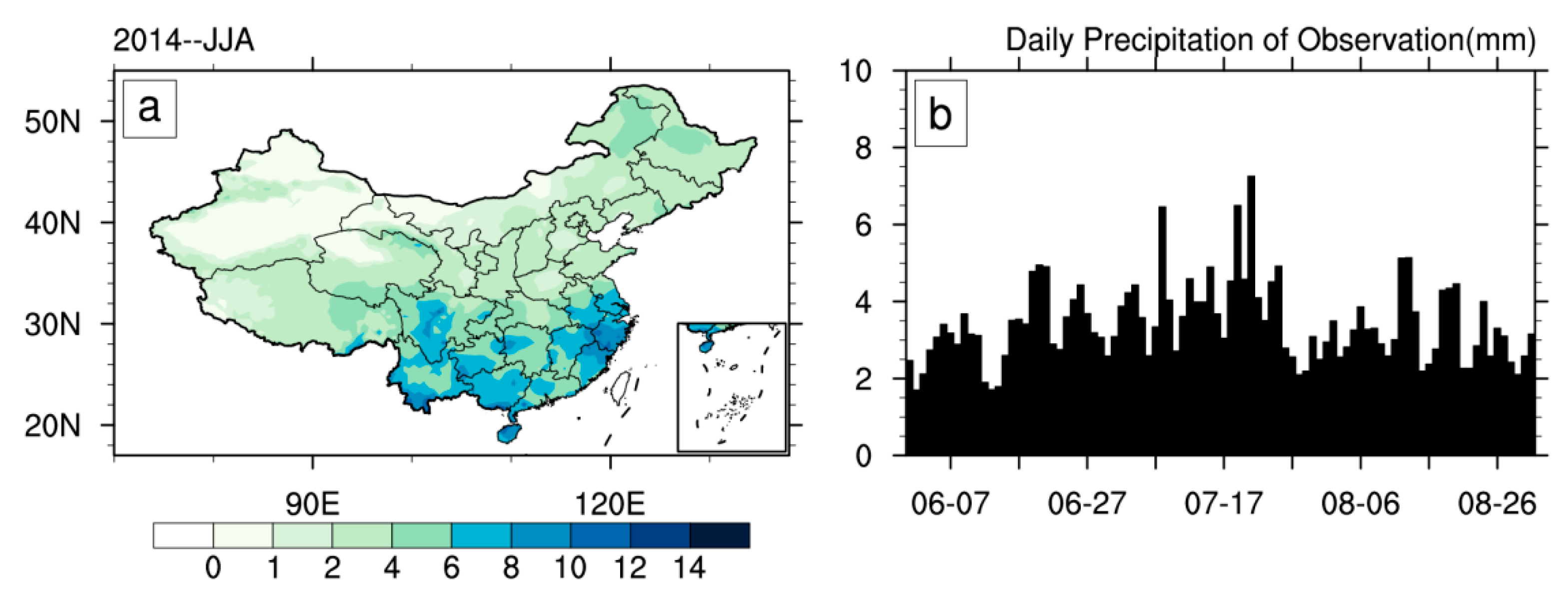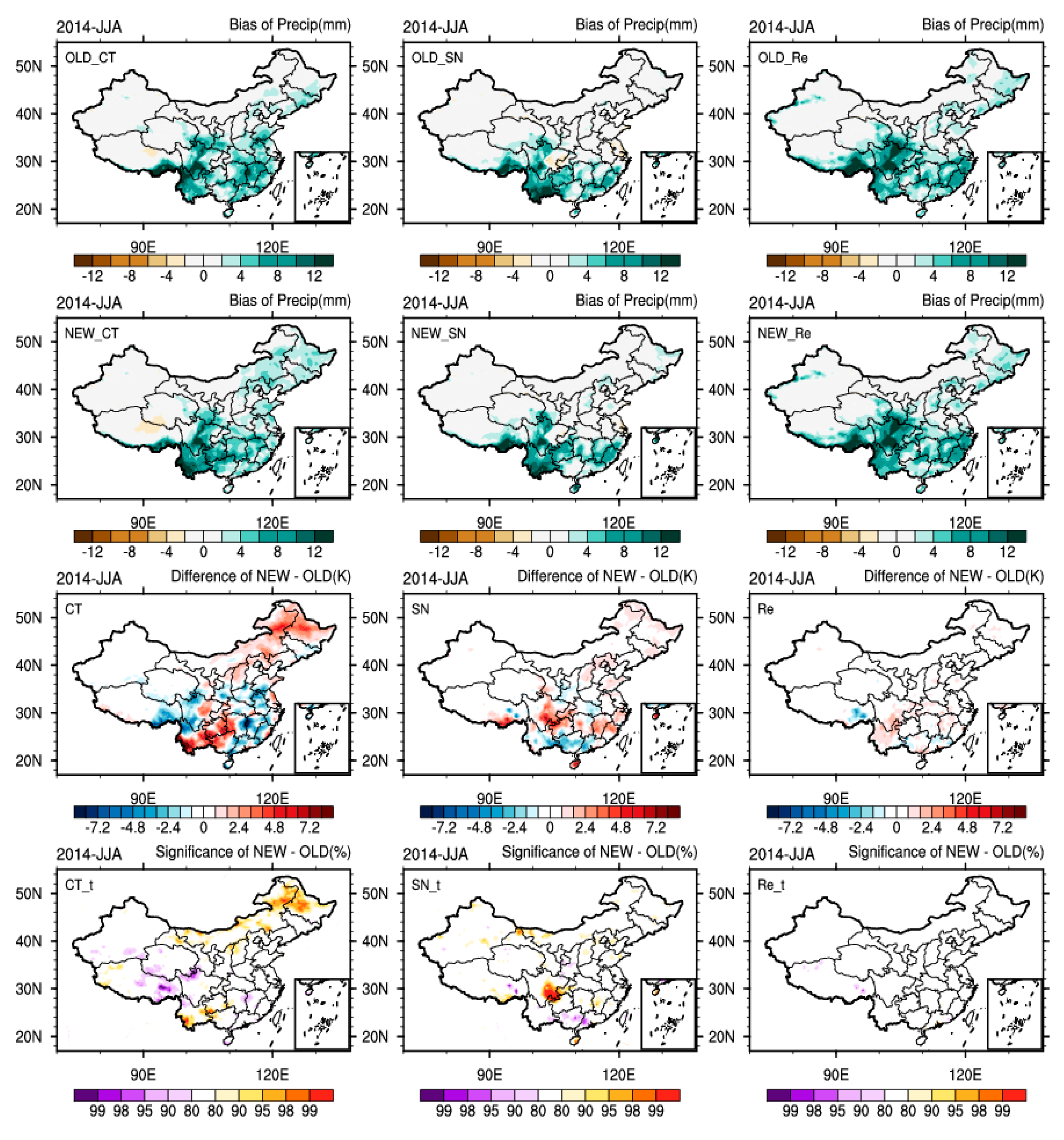In the OLD group, the Re method is more advantageous than the SN method by test of statistical significance (Table 4 and Table 5). The precipitation verification shows that all three methods overestimate precipitation south of the Yangtze River. The Re runs feature the most obvious overestimations in the southeast TP, followed by the CT method; the SN method, which constrains error growth in large-scale circulations during long simulations, shows the smallest bias in precipitation magnitude and distribution. The SN method also maintains consistency with the large-scale behavior of the ERA-Interim forcing data higher in the atmosphere.

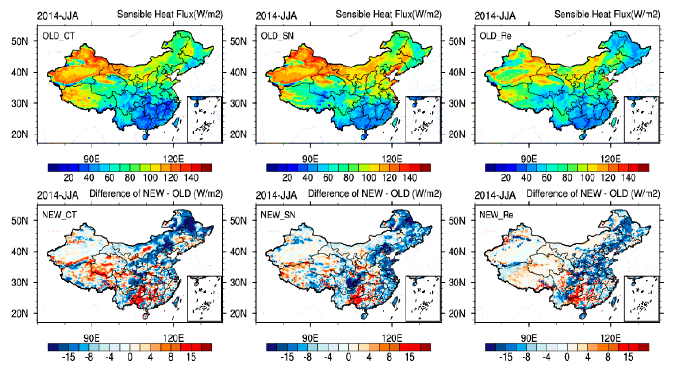
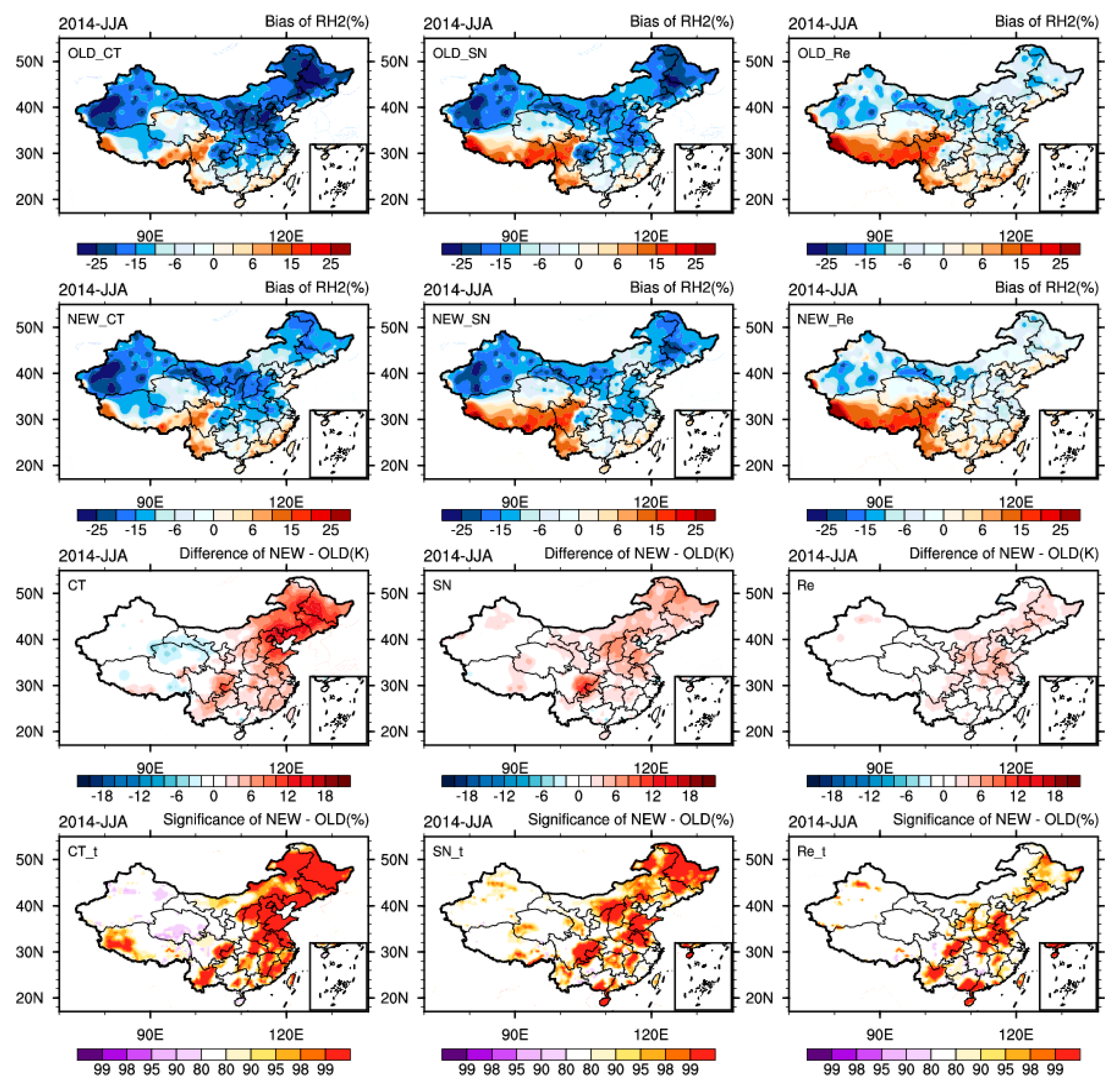
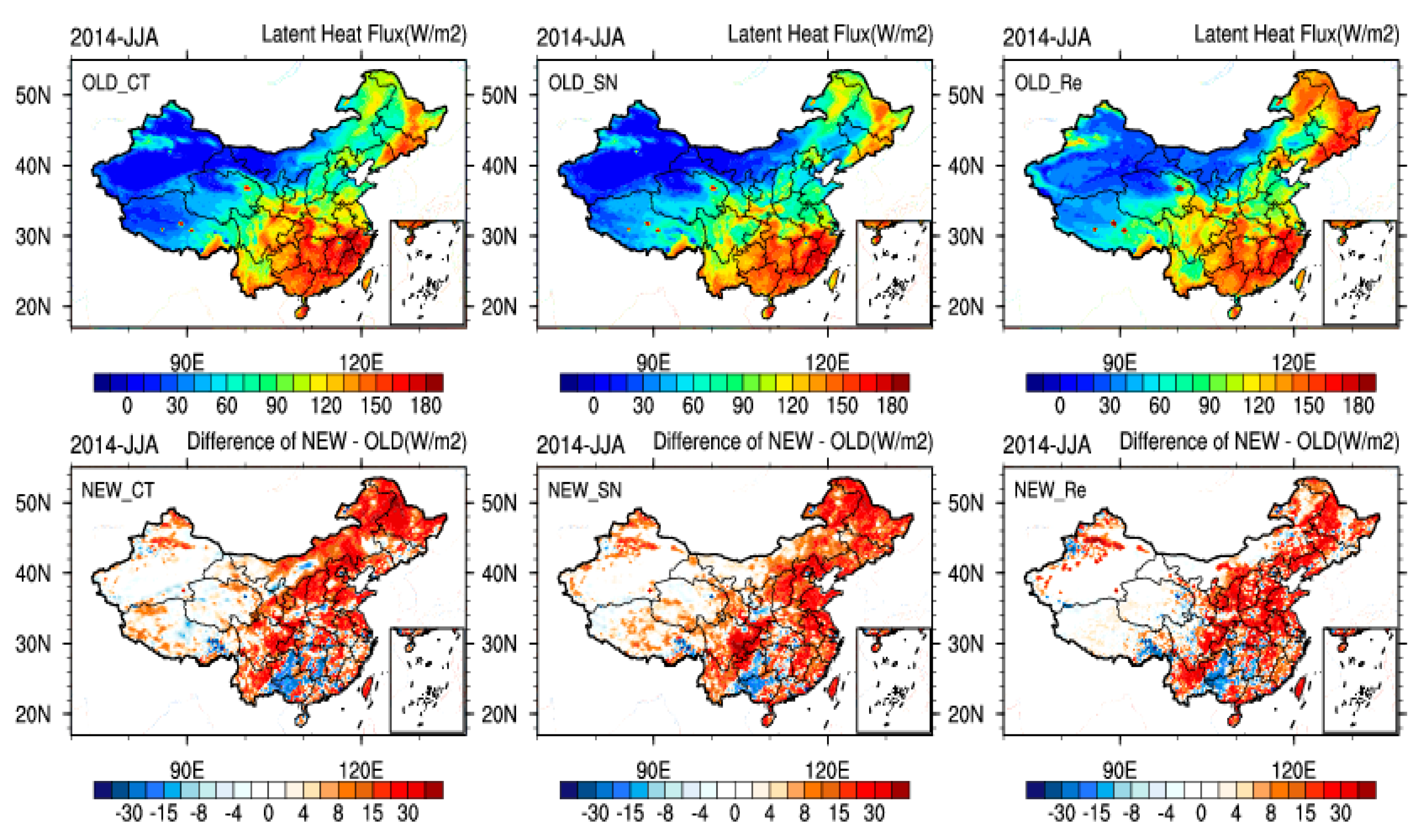
The default land use and vegetation fraction in the WRF do not accurately reflect the land surface conditions during the analysis period. Compared with the OLD group, the ME, RMSE simulations of temperature and relative humidity are significantly improved in NEW_CT/NEW_SN experiments, and ME is improved in NEW_Re experiments. This effect is especially conspicuous in the CT method, followed by the SN and Re methods. Because the CT method is less constrained by forcing fields in the continuous integration process and is allowed the model to develop freely. The 2 m temperature and relative humidity are more sensitive to changes in land surface information. Therefore, the CT simulations are improved after accurate land surface information is introduced. However, because precipitation is affected by the large-scale circulation field, there is no obvious improvement in precipitation.

The results support this study’s hypothesis that updating accurate land surface information would affect downscaling performance. However, the benefits of updated land surface information for SN and Re methods are not as significant as CT. There are two possible reasons for this. First, when the large-scale information is nudged, the development of small-scale information generated by the land surface information changes is restricted in SN. However, the reason for this is still uncertain, and this topic needs additional research and analysis. Second, in the Re method, the initial field is frequently updated and fails to reflect the cumulative effect of updating land surface information on the climate field. Future studies will explore a method to reduce this drawback.

The heterogeneity and complexity of a land surface is characterized by various land surface information parameters in the model land surface processes. Therefore, in order to more accurately reflect land-atmosphere interactions, accurate initial land surface information is introduced in a regional model to obtain more valuable small-scale regional information. This, in turn, achieves greater added value through dynamical downscaling, which is a cost-effective and practical approach to improve the dynamical downscaling performance of different methods. Therefore, it is necessary to create dynamically accordant initial land surface data sets consistent with the downscaling experiment analysis period.

References

1. IPCC. Climate Change 2013: The Physical Science Basis. Contribution of Working Group I to the Fifth Assessment Report of the Intergovernmental Panel on Climate Change; Cambridge University Press: Cambridge, UK, 2013. [Google Scholar]
2. Giorgi, F. Regional climate modeling: Status and perspectives. J. Phys. IV 2006, 139, 101–118. [Google Scholar] [CrossRef]
3. Heikkilä, U.; Sandvik, A.; Sorteberg, A. Dynamical downscaling of ERA-40 in complex terrain using the WRF regional climate model. Clim. Dyn. 2011, 37, 1551–1564. [Google Scholar]
4. White, C.J.; McInnes, K.L.; Cechet, R.P.; Corney, S.P.; Grose, M.R.; Holz, G.K.; Katzfey, J.J.; Bindoff, N.L. On regional dynamical downscaling for the assessment and projection of temperature and precipitation extremes across tasmania, australia. Clim. Dyn. 2013, 41, 3145–3165. [Google Scholar] [CrossRef]
5. Sun, X.; Xue, M.; Brotzge, J.; McPherson, R.A.; Hu, X.-M.; Yang, X.-Q. An evaluation of dynamical downscaling of central plains summer precipitation using a WRF-based regional climate model at a convection-permitting 4 km resolution. J. Geophys. Res. Atmos. 2016, 121, 13801–13825. [Google Scholar] [CrossRef]
6. Lo, J.C.-F.; Yang, Z.-L.; Pielke, R.A. Assessment of three dynamical climate downscaling methods using the weather research and forecasting (WRF) model. J. Geophys. Res. 2008, 113. [Google Scholar] [CrossRef]
7. Rockel, B.; Castro, C.L.; Pielke, R.A.; von Storch, H.; Leoncini, G. Dynamical downscaling: Assessment of model system dependent retained and added variability for two different regional climate models. J. Geophys. Res. 2008, 113. [Google Scholar] [CrossRef]
8. Racherla, P.N.; Shindell, D.T.; Faluvegi, G.S. The added value to global model projections of climate change by dynamical downscaling: A case study over the continental US using the GISS—ModelE2 and WRF models. J. Geophys. Res. Atmos. 2012, 117. [Google Scholar] [CrossRef]
9. Rummukainen, M. Added value in regional climate modeling. Wires Clim. Chang. 2016, 7, 145–159. [Google Scholar] [CrossRef]
10. Stauffer, D.R.; Seaman, N.L.; Binkowski, F.S. Use of four-dimensional data assimilation in a limited-area mesoscale model Part II: Effects of data assimilation within the planetary boundary layer. Mon. Weather Rev. 1991, 119, 734–754. [Google Scholar] [CrossRef]
11. Von Storch, H.; Langenberg, H.; Feser, F. A spectral nudging technique for dynamical downscaling purposes. Mon. Weather Rev. 2000, 128, 3664–3673. [Google Scholar] [CrossRef]
12. Miguez-Macho, G.; Stenchikov, G.L.; Robock, A. Spectral nudging to eliminate the effects of domain position and geometry in regional climate model simulations. J. Geophys. Res. Atmos. 2004, 109, D13. [Google Scholar] [CrossRef]
13. Barstad, I.; Sorteberg, A.; Flatøy, F.; Déqué, M. Precipitation, temperature and wind in Norway: Dynamical downscaling of ERA40. Clim. Dyn. 2009, 33, 769–776. [Google Scholar] [CrossRef]
14. Gula, J.; Peltier, W.R. Dynamical downscaling over the great lakes basin of north america using the WRF regional climate model: The impact of the great lakes system on regional greenhouse warming. J. Clim. 2011, 25, 7723–7742. [Google Scholar] [CrossRef]
15. Stauffer, D.R.; Seaman, N.L. Use of four-dimensional data assimilation in a limited-area mesoscale model. Part I: Experiments with synoptic-scale data. Mon. Weather Rev. 1990, 118, 1250–1277. [Google Scholar] [CrossRef]
16. Waldron, K.M.; Paegle, J.; Horel, J.D. Sensitivity of a spectrally filtered and nudged limited-area model to outer model options. Mon. Weather Rev. 1996, 124, 529. [Google Scholar] [CrossRef]
17. Pleim, J.; Young, J.; Wong, D.; Gilliam, R.; Otte, T.; Mathur, R. Two-way coupled meteorology and air quality modeling. Nato Secur. Sci. 2008, 235–242. [Google Scholar] [CrossRef]
18. Liu, P.; Tsimpidi, A.P.; Hu, Y.; Stone, B.; Russell, A.G.; Nenes, A. Differences between downscaling with spectral and grid nudging using WRF. Atmos. Chem. Phys. 2012, 12, 3601–3610. [Google Scholar] [CrossRef]
19. Bowden, J.H.; Otte, T.L.; Nolte, C.G.; Otte, M.J. Examining interior grid nudging techniques using two-way nesting in the WRF model for regional climate modeling. J. Clim. 2012, 25, 2805–2823. [Google Scholar] [CrossRef]
20. Spero, T.L.; Otte, M.J.; Bowden, J.H.; Nolte, C.G. Improving the representation of clouds, radiation, and precipitation using spectral nudging in the weather research and forecasting model. J. Geophys. Res. Atmos. 2014, 119, 11,682–11,694. [Google Scholar] [CrossRef]
21. Castro, C.L.; Pielke, R.A.; Leoncini, G. Dynamical downscaling: Assessment of value retained and added using the regional atmospheric modeling system (RAMS). J. Geophys. Res. Atmos. 2005, 110. [Google Scholar] [CrossRef]
22. Mai, X.P.; Ma, Y.; Yang, Y.; Li, D.; Qiu, X. Impact of Grid Nudging Parameters on Dynamical Downscaling during Summer over Mainland China. Atmosphere 2017, 8, 184. [Google Scholar] [CrossRef]
23. Miguezmacho, G.; Stenchikov, G.L.; Robock, A. Regional climate simulations over North America: Interaction of local processes with improved large-scale flow. J. Clim. 2005, 18, 1227–1246. [Google Scholar] [CrossRef]
24. Ma, Y.; Yang, Y.; Mai, X.; Qiu, C.; Long, X.; Wang, C. Comparison of analysis and spectral nudging techniques for dynamical downscaling with the WRF model over China. Adv. Meteorol. 2016, 2016, 1–16. [Google Scholar] [CrossRef]
25. Qian, J.-H.; Seth, A.; Zebiak, S. Reinitialized versus continuous simulations for regional climate downscaling. Mon. Weather Rev. 2003, 131, 2857–2874. [Google Scholar] [CrossRef]
26. Caldwell, P.; Chin, H.-N.S.; Bader, D.C.; Bala, G. Evaluation of a WRF dynamical downscaling simulation over california. Clim. Chang. 2009, 95, 499–521. [Google Scholar] [CrossRef]
27. Lucas-Picher, P.; Boberg, F.; Christensen, J.H.; Berg, P. Dynamical downscaling with reinitializations: A method to generate finescale climate datasets suitable for impact studies. J. Hydrometeorol. 2013, 14, 1159–1174. [Google Scholar] [CrossRef]
28. Koster, R.D.; Mahanama, S.P.P.; Yamada, T.J.; Balsamo, G.; Berg, A.A.; Boisserie, M.; Dirmeyer, P.A.; Doblas-Reyes, F.J.; Drewitt, G.; Gordon, C.T.; et al. Contribution of land surface initialization to subseasonal forecast skill: First results from a multi-model experiment. Geophys. Res. Lett. 2010, 37. [Google Scholar] [CrossRef]
29. Bagley, J.E.; Kueppers, L.M.; Billesbach, D.P.; Williams, I.N.; Biraud, S.C.; Torn, M.S. The influence of land cover on surface energy partitioning and evaporative fraction regimes in the us southern great plains. J. Geophys. Res. Atmos. 2017, 122, 5793–5807. [Google Scholar] [CrossRef]
30. Nicholson, S. Land surface processes and Sahel climate. Rev. Geophys. 2000, 38, 117–139. [Google Scholar] [CrossRef]
31. Kanamitsu, M.; Mo, K.C. Dynamical effect of land surface processes on summer precipitation over the southwestern United States. J. Clim. 2003, 16, 496–509. [Google Scholar] [CrossRef]
32. Hong, S.Y.; Lim, J.O.J. The WRF single-moment 6-class microphysics scheme (WSM6). J. Korean Meteor. Soc. 2006, 42, 129–151. [Google Scholar]
33. Moalafhi, D.B.; Evans, J.P.; Sharma, A. Evaluating global reanalysis datasets for provision of boundary conditions in regional climate modelling. Clim. Dyn. 2016, 146, 1–19. [Google Scholar] [CrossRef]
34. Rummukainen, M. State-of-the-art with regional climate models. Wiley Interdisciplin. Rev. Clim. Chang. 2010, 1, 82–96. [Google Scholar] [CrossRef]
35. Choi, H.I. Use of sensor imagery data for surface boundary conditions in regional climate modeling. Sensors 2011, 11, 6728–6742. [Google Scholar] [CrossRef] [PubMed]
36. Tao, Z.; Santanello, J.A.; Chin, M.; Zhou, S. Effect of land cover on atmospheric processes and air quality over the continental united states—A NASA unified WRF (NU-WRF) model study. Atmos. Chem. Phys. 2013, 13, 6207–6226. [Google Scholar] [CrossRef]
37. Deng, X.; Shi, Q.; Zhang, Q.; Shi, C.; Yin, F. Impacts of land use and land cover changes on surface energy and water balance in the Heihe river basin of China, 2000–2010. Phys. Chem. Earth Parts A/B/C 2015, 79–82, 2–10. [Google Scholar] [CrossRef]
38. Loveland, T.R.; Merchant, J.W.; Brown, J.F.; Ohlen, D.O.; Reed, B.C.; Olson, P.; Hutchinson, J. Seasonal land-cover regions of the United States. Ann. Assoc. Am. Geogr. 1995, 85, 339–355. [Google Scholar] [CrossRef]
39. Friedl, M.A.; Sulla-Menashe, D.; Tan, B.; Schneider, A.; Ramankutty, N.; Sibley, A.; Huang, X. Modis collection 5 global land cover: Algorithm refinements and characterization of new datasets. Remote Sens. Environ. 2010, 114, 168–182. [Google Scholar] [CrossRef]
40. Liu, J.Y.; Liu, M.L.; Zhuang, D.F.; Deng, X.Z. Study on the spatial pattern of land-use change in China during 1995–2000. Sci. China Ser. D Earth Sci. 2003, 46, 373–384. [Google Scholar]
41. Gong, P. Accuracy assessment of global land cover datasets based on global field stations. Prog. Nat. Sci. 2009, 19, 754–759. [Google Scholar]
42. He, J.J.; Yu, Y.; Liu, N.; Zhao, S.P.; Chen, J.B. Impact of land surface information on WRF’s performance in complex terrain area. Chin. J. Atmos. Sci. 2014, 38, 484–498. [Google Scholar]
43. Wu, B.F.; Yuan, Q.; Yan, C.; Wang, Z.; Yu, X.; Li, A.; Ma, R.H.; Huang, J.L.; Chen, J.S.; Chang, C.; et al. Land cover changes of China from 2000 to 2010. Quat. Sci. 2014, 34, 723–731. [Google Scholar]
44. Gutman, G.; Ignatov, A. The derivation of the green vegetation fraction from NOAA/AVHRR data for use in numerical weather prediction models. Int. J. Remote Sens. 1998, 19, 1533–1543. [Google Scholar] [CrossRef]
45. Zhao, H.Q. Research on the Vegetation Coverage Changes of China Based on SPOT-4/VEGETATION Data. Geomat. Spat. Inf. Technol. 2010, 1, 051. [Google Scholar]
46. Li, D.Q.; Wen, X.H.; Duan, Y.X.; Zhou, X.S.; Yang, S. A comparison study of fraction of green vegetation coverage estimated using modis products and default data used in WRF model. J. Meteorol. Environ. 2015, 31, 26–34. Available online: http://xueshu.baidu.com/s?wd=MODIS+%E4%BA%A7%E5%93%81%E5%8F%8D%E6%BC%94%E4%B8%8E+W%EF%BC%B2F+%E6%A8%A1%E5%BC%8F%E9%BB%98%E8%AE%A4+%E6%A4%8D%E8%A2%AB%E8%A6%86%E7%9B%96%E5%BA%A6%E5%AF%B9%E6%AF%94%E7%A0%94%E7%A9%B6&tn=SE_baiduxueshu_c1gjeupa&cl=3&ie=utf-8&bs=doi%3A10.3969%2Fj.issn.1673-503X.2015.04.005&f=8&rsv_bp=1&rsv_sug2=0&sc_f_para=sc_tasktype%3D{firstSimpleSearch}&rsv_spt=3&rsv_n=2 (assessed on 22 February 2018). [CrossRef]
47. Skamarock, W.C.; Klemp, J.B.; Dudhia, J.; Gill, D.O.; Barker, D.M.; Duda, M.G.; Huang, X.Y.; Wang, W.; Powers, J.G. A description of the advanced research WRF Version 3. In NCAR Technical Note; NCAR: Boulder, CO, USA, 2008; TN-475+STR. [Google Scholar]
48. Lim, K.S.S.; Hong, S.Y. Development of an effective double-moment cloud microphysics scheme with prognostic cloud condensation nuclei (CCN) for weather and climate models. Mon. Weather Rev. 2010, 138, 1587–1612. [Google Scholar] [CrossRef]
49. Collins, W.D.; Rasch, P.J.; Boville, B.A.; Hack, J.J.; Mccaa, J.R.; Williamson, D.L.; Briegleb, K.J.T.B. Description of the NCAR community atmosphere model (CAM 3.0). Natl. Cent. Atmos. Res. Ncar Koha Opencat 2004. [Google Scholar]
50. Hong, S.Y.; Noh, Y.; Dudhia, J. A new vertical diffusion package with an explicit treatment of entrainment processes. Mon. Weather Rev. 2006, 134, 2318. [Google Scholar] [CrossRef]
51. Jiménez, P.A.; Dudhia, J.; González-Rouco, J.F.; Navarro, J.; Montávez, J.P.; García-Bustamante, E. A revised scheme for the WRF surface layer formulation. Mon. Weather Rev. 2012, 140, 898–918. [Google Scholar] [CrossRef]
52. Chen, F.; Dudhia, J. Coupling an advanced land surface hydrology model with the Penn State NCAR MM5 modeling system. Part II: Preliminary model validation. Mon. Weather Rev. 2001, 129, 569–585. [Google Scholar] [CrossRef]
53. Gu, H.; Jin, J.; Wu, Y.; Ek, M.B.; Subin, Z.M. Calibration and validation of lake surface temperature simulations with the coupled WRF-lake model. Clim. Chang. 2015, 129, 471–483. [Google Scholar] [CrossRef]
54. Oleson, K.W.; Lawrence, D.M.; Bonan, G.B. Technical description of version 4.5 of the community land model (CLM). NCAR tech. Note NCAR/TN-503+STR. National Center for Atmospheric Research: Boulder, CO, USA. Geophys. Res. Lett. 2013, 37, 256–265. [Google Scholar]
55. Liang, S.H.; Chen, J.; Jin, X.M.; Wan, L.; Gong, B. Regularity of vegetation coverage changes in the Tibetan Plateau over the last 21 years. Adv. Earth Sci. 2007, 22, 33–40. [Google Scholar]
56. Zhang, L.Z.; Li, M.; Wu, Z.F.; Liu, Y.J. Vegetation cover change and its mechanism in northeast China based on SPOT/NDVI data. J. Arid Land Resour. Environ. 2011, 25, 171–175. [Google Scholar]
57. Zeng, X.; Dickinson, R.E.; Walker, A.; Shaikh, M.; DeFries, R.S.; Qi, J. Derivation and evaluation of global 1-km fractional vegetation cover data for land modeling. J. Appl. Meteorol. 2000, 39, 826–839. [Google Scholar] [CrossRef]
58. Miller, J.; Barlage, M.; Zeng, X.; Wei, H.; Mitchell, K.; Dan, T. Sensitivity of the NCEP/NOAH land surface model to the modis green vegetation fraction data set. Geophys. Res. Lett. 2006, 33, 338–345. [Google Scholar] [CrossRef]
Figure 1. Configuration of Weather Research and Forecasting (WRF) model domain and topography height; the color scale refers to elevation.
Atmosphere 09 00101 g001
Figure 2. Distribution of OLD_LU and NEW_LU. The color scale refers to land category.
Atmosphere 09 00101 g002
Figure 3. Monthly distribution of the WRF default vegetation fraction (OLD_VF) and the updated vegetation fraction (NEW_VF) calculated by MODIS data in summer (June, July, August, JJA) 2014.
Atmosphere 09 00101 g003
Figure 4. Bias distribution of the daily averaged temperature (T2) in summer 2014. The first row (continuous integration (CT), spectral nudging (SN), and re-initialization (Re); OLD_CT, OLD_SN, OLD_Re) contains the OLD group, the second row (NEW_CT, NEW_SN, NEW_Re) contains the NEW group. The third row (CT, SN, Re) is the difference between simulation of NEW and OLD group. The last row (CT_t, SN_t, Re_t) is the statistical significance of the difference between NEW and OLD group for each grid 92-day simulations of temperature correspond to CT, SN, and Re, respectively. The left (OLD_CT, NEW_CT, CT), middle (OLD_SN, NEW_SN, SN), and right (OLD_Re, NEW_Re, Re) columns correspond to the CT, SN, and Re simulations, respectively.
Atmosphere 09 00101 g004
Figure 5. Time series of spatial ME (a); root means square error (RMSE) (b); and cc (c) for daily 2 m temperature in the summer of 2014 over China. The top (NEW_CT, OLD_CT), middle (NEW_SN, OLD_SN), and bottom (NEW_Re, OLD_Re) rows correspond to the CT, SN, and Re simulations, respectively.
Atmosphere 09 00101 g005
Figure 6. Probability density distribution of daily temperature MB for each grid and each day in summer 2014.
Atmosphere 09 00101 g006
Figure 7. Same as Figure 4, but for 2 m relative humidity (RH2).
Atmosphere 09 00101 g007
Figure 8. Time series of spatial ME (a); root means square error (RMSE) (b); and cc (c) for daily 2 m relative humidity in the summer of 2014 over China. The top (NEW_CT, OLD_CT), middle (NEW_SN, OLD_SN), and bottom (NEW_Re, OLD_Re) rows correspond to the CT, SN, and Re simulations, respectively.
Atmosphere 09 00101 g008
Figure 9. Same as Figure 6, but for 2 m relative humidity.
Atmosphere 09 00101 g009
Figure 10. Spatial distribution with time-averaged (all days) (a) and times series with spatial-averaged (all grid points) (b) of daily accumulated precipitation from observation data in summer, 2014.
Atmosphere 09 00101 g010
Figure 11. Same as Figure 4, but for precipitation (Precip).
Atmosphere 09 00101 g011
Figure 12. Time series of spatial ME (a); root means square error (RMSE) (b); and cc (c) for daily accumulated precipitation in the summer of 2014 over China. The top (NEW_CT, OLD_CT), middle (NEW_SN, OLD_SN), and bottom (NEW_Re, OLD_Re) rows correspond to the CT, SN, and Re simulations, respectively. 2014.
Atmosphere 09 00101 g012
Figure 13. Same as Figure 6, but for daily accumulated precipitation in summer, 2014.
Atmosphere 09 00101 g013
Figure 14. Distribution of averaged sensible heat flux (W m−2) from OLD simulation in summer (OLD_CT, OLD_SN, OLD_Re), the corresponding differences between NEW and OLD simulations (NEW_CT, NEW_SN, NEW_Re), the left (OLD_CT, NEW_CT), middle (OLD_SN, NEW_SN), and right (OLD_Re, NEW_Re) columns correspond to the CT, SN, and Re simulations, respectively.
Atmosphere 09 00101 g014
Figure 15. Same as Figure 14, but for the latent heat flux (W m−2).
Atmosphere 09 00101 g015