Vortex Motion State of the Dry Atmosphere with Nonzero Velocity Divergence


Department of General and Theoretical Physics, Institute of Mathematics and Natural Sciences, North Caucasus Federal University, 1 Pushkin Street, Stavropol 355009, Russia
*
Author to whom correspondence should be addressed.
Atmosphere 2018, 9(2), 61; https://doi.org/10.3390/atmos9020061
Submission received: 25 December 2017
/
Revised: 7 February 2018
/
Accepted: 8 February 2018
/
Published: 10 February 2018
(This article belongs to the Special Issue Selected Papers from The 2nd International Electronic Conference on Atmospheric Sciences)
Abstract
:In the present work, an analytical model of the vortex motion basic state of the dry atmosphere with nonzero air velocity divergence is constructed. It is shown that the air parcel moves along the open curve trajectory of spiral geometry. It is found that for the case of nonzero velocity divergence, the atmospheric basic state presents an unlimited sequence of vortex cells transiting from one to another. On the other hand, at zero divergence, the basic state presents a pair of connected vortices, and the trajectory is a closed curve. If in some cells the air parcel moves upward, then in the adjacent cells, it will move downward, and vice versa. Upon reaching the cell’s middle height, the parcel reverses the direction of rotation. When the parcel moves upward, the motion is of anticyclonic type in the lower part of the vortex cell and of cyclonic type in the upper part. When the parcel moves downward, the motion is of anticyclonic type in the upper part of the vortex cell and of cyclonic type in the lower part.
1. Introduction
It is well known that the geostrophic state is a two-dimensional basic state for large-scale atmospheric motion [1,2,3]. In the geostrophic state, the motion is nondivergent, and thus, there is no vertical motion [4,5]. However, in reality, the atmospheric motions are three-dimensional, and the motion is certainly upward or downward as a result of various reasons. Spiral structures of vortices in the atmosphere in different scales form in these cases [6]. A typical three-dimensional basic state is cyclonic vorticity with rising motion due to surface convergence and anticyclonic vorticity as well as sinking motion due to surface divergence. Exact solutions of the Navier–Stokes equations for a three-dimensional vortex have been discovered [7,8,9,10,11]; of particular interest is Sullivan’s two-cell vortex solution, because the flow not only spirals in toward the axis and out along it, but it also has a region of reverse flow near the axis.
It should be noted that there are a large number of works dedicated to the theoretical study of atmospheric vortices. However, most of these are concerned with the numerical solution of the atmospheric motion equations. Analytical models of steady-state vortexes in the atmosphere have been examined in fewer studies (e.g., [12,13]). In [14,15,16], three-dimensional atmospheric vortex motion is analyzed by considering the primitive dynamic and thermodynamic equations, including the Coriolis, pressure gradient and viscous forces. It should be noted that nondivergent motion has been studied in [14,15,16]. Furthermore, a strong assumption of the model in [14,15,16] is that the viscous friction force linearly depends on the velocity. In this paper, we further develop the theoretical model of the vortex motion state of the atmosphere. The main goal of the study is to refine the model by taking into account the nonzero velocity divergence term in the equations of motion. In addition, we use a more general expression for the friction force in the form of proportionality to the velocity Laplacian.
2. Main Equations
In the local coordinate system, the atmospheric state is described by the set of Equations (1)–(5):
Here, ; and are the air temperatures of the disturbed and undisturbed atmosphere correspondingly; are the projections of the air velocity on the axes; is the air density; is the air pressure; are the projections of the earth’s angular velocity on the axes; is the air kinematic viscosity; is the air temperature conductivity coefficient; is the air thermal expansion coefficient, where ; is the temperature vertical gradient; is the “autoconvective vertical gradient”; is the acceleration of gravity; is the dry-air specific gas constant. The x-axis is tangential to the parallel line in the direction of the earth’s rotation, the y-axis is tangential to the meridian in the direction from the equator to the North Pole, and the z-axis is perpendicular to the earth’s surface. Thus, . Here we neglect the geoidal shape of the earth and assume it to be spherical. The air density has the form ; the static density decreases with height by the exponential law. Equation (5) has been obtained by substitution of the density expression into the continuity equation.
The basic state of the atmosphere is assumed to be in hydrostatic balance:
We let the atmospheric parameters have the form of perturbation of the static state:
Here, is the dry-air adiabatic temperature gradient.
It is convenient to convert the equations into dimensionless form. The length scales for horizontal and vertical directions are taken as L and H, the velocity scale in horizontal directions is U, the time scale is L/U, the vertical velocity scale is HU/L, the scale for pressure is , and the temperature scale is . At the same time, we set , (Reynolds number), (Richardson number), N (Brunt–Väisälä frequency, ), (Prandtl number), (Rossby number), and . If we drop the advective terms in Equations (1)–(5) and assume (i.e., L = H), then the set of equations can be written as
Differentiating with respect to y and x and subtracting Equation (1) from Equation (2), we obtain
Here
are the vertical vorticity and horizontal divergence, correspondingly.
Analogously, differentiating and summing Equations (6) and (7), we obtain
Thus we have
We assume that the three-dimensional atmospheric state is time independent and stationary. Neglecting the advective terms, Equations (11)–(15) can be transformed:
Excluding , , and , we obtain the required partial differential equation:
where
Ra is the Rayleigh number, and Ta is the Taylor number.
3. Solution of the Main Equations
Following the previous studies [7,8,9,10,11,14,15,16], we assume that has the form
where k is the wave number; is the initial phase determining the initial value of the air vertical velocity component at ; n is the mode number equal to the number of wave lengths within the characteristic length scale L. In fact, n is the number of the vortex cell on the vertical axis; hereafter we assume that n = 1.
Substituting Equation (23) into Equation (21), we obtain
The functional form of the zonal velocity components differs from the corresponding expressions in the previous studies [7,8,9,10,11,14,15,16] because of the fact that the velocity divergence is nonzero. Thus, we seek the expression of u in the form:
Substituting, we obtain
From here we have
We also have
Assuming and , we obtain, for the Brunt–Väisälä frequency, or
From here it follows that the critical value of the vertical temperature gradient is close to the value of the dry-air adiabatic gradient.
Finally
Figure 1 shows the velocity field in accordance with Equations (24)–(26). In all calculations, we assume that . It is seen that the air parcel motion has a three-dimensional vortex structure.
Figure 2 shows the air parcel trajectory numerically calculated in accordance with Equations (24)–(26). As is seen from Figure 2, the air parcel trajectory is an unclosed curve. In other words, the parcel passes from one vortex cell to another. It is also seen that while the air parcel in the lower level is spirally converged towards the center, the air is lifted up. After the air parcel arrives at high level, the air parcel is spirally diverged outwards. In the same way, if the air parcel is spirally converged towards the center at the upper level, then it moves downwards to the lower level and diverges. Thus, one can see that the basic state of the atmosphere in the case of nonzero divergence is a sequence of connected vortex cells. On the other hand, at zero divergence, the air parcel trajectory is a closed curve and the atmospheric state is a pair of connected vortices, as has been shown in previous studies.
It can be seen from Equation (20) that if the velocity divergence is equal to zero, then the vertical velocity component has the following height dependence:
where is the initial value of velocity at the earth’s surface at . From here it follows that at zero initial velocity and zero divergence, the upward air movement is absent. Letting the velocity divergence be nonzero and constant, then from Equation (20), we have
One can see that the upward air movement in the lower atmosphere is only possible at negative divergence (D < 0).
Equation (11) represents a vortex transport (diffusion) equation with a source of the form . It follows that if and (convergent horizontal air motion in the lower atmosphere, D < 0), then and . This means that the vortex has a cyclonic vorticity in the lower atmosphere. In analogy, Equation (12) represents a divergence transport (diffusion) equation with a source of the form . It follows from Equation (17) that if the velocity divergence is constant and negative (D < 0), then . From here it follows that if . This means that the pressure is low at the center of the cyclonic vortex.
Equations (18) and (19) relate the three-dimensional flow pattern and the temperature field. At positive vertical velocity, it follows from Equation (19) that . This means that the cyclonic vortex center is heated, that is, the temperature maximum is at the cyclonic vortex center.
The obtained solution describes the basic state of the atmosphere, which is the vortex motion state. It can be demonstrated that the traditional geostrophic state is a limiting case of the vortex motion state. Indeed, at , that is, when the viscosity is negligible, and , from Equation (16), one can obtain that . From Equation (18) it follows that
For the stationary state, from Equations (6)–(10), one can obtain the components of the geostrophic velocity:
These expressions coincide with the expressions for the geostrophic state of the atmosphere [1,2,3].
We return to the system of Equations (16)–(20). The expression for the velocity divergence can be obtained from Equation (20):
From here it follows that the horizontal divergence reverses sign at a height of
If within a layer the horizontal divergence is negative and the convergence takes place, then within the layer , the horizontal divergence will be positive, and vice versa. This is a manifestation of Dines’s compensation principle. Thus, one can see that this principle takes place not only at zero total velocity divergence but also at nonzero total divergence.
The expression for the temperature disturbance can be obtained from Equation (19):
The expression for the pressure disturbance can be obtained from Equation (18):
The expression for the vorticity can be obtained from Equation (17):
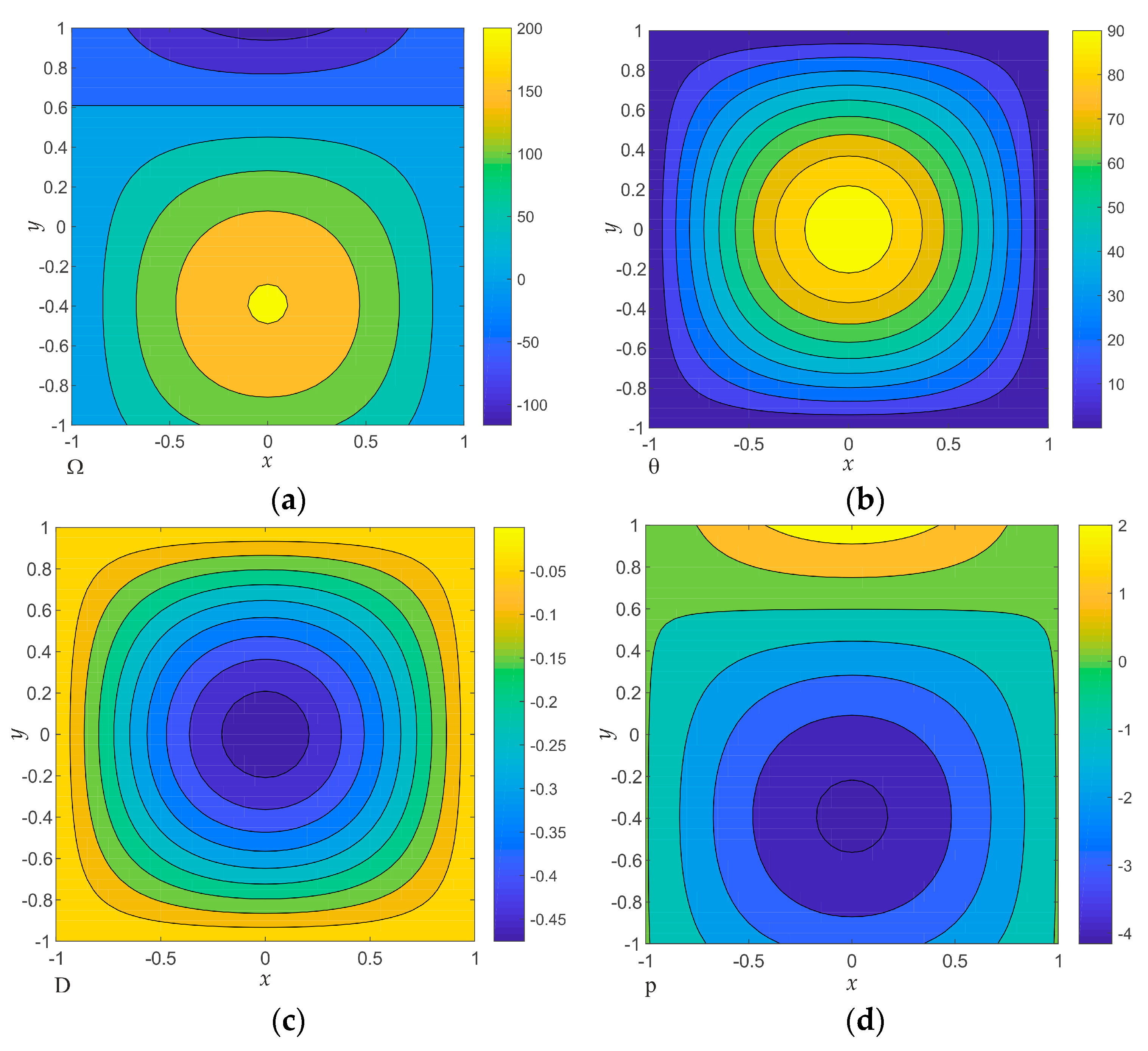
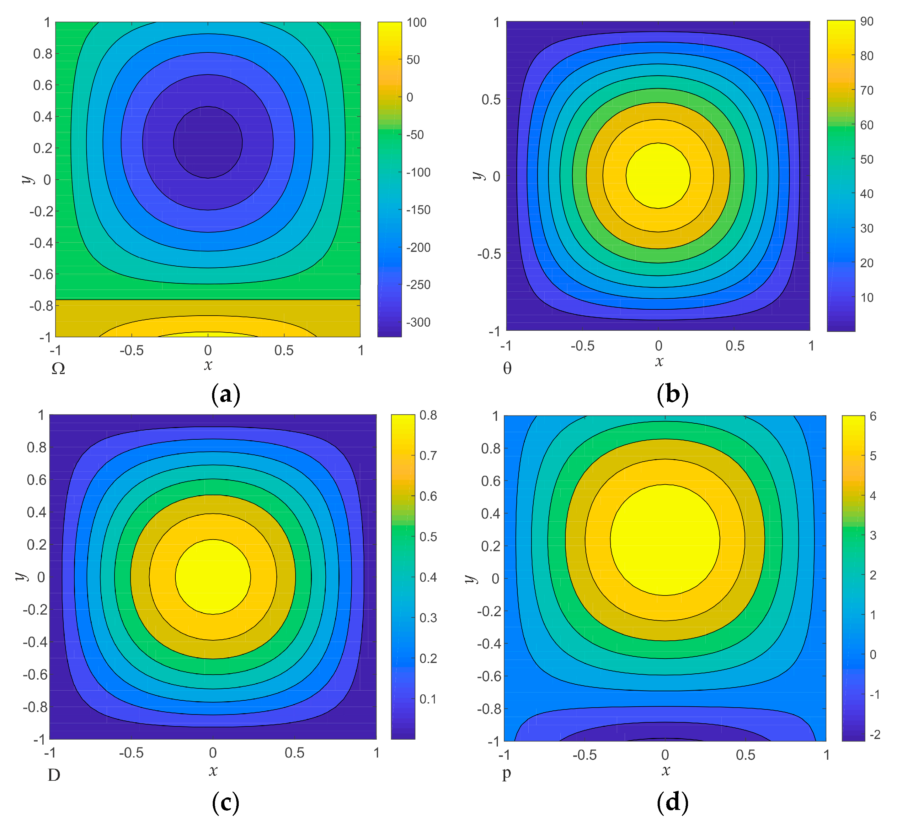
Figure 3 and Figure 4 show the fields of vorticity, temperature, divergence, and pressure at the altitudes (lower part of the vortex cell) and (upper part of the vortex cell), correspondingly. As is seen, if the motion field in the lower part of the cell has a cyclonic vorticity, then in the upper part, it has an anticyclonic vorticity, and vice versa. The divergence changes in sign at the transition from one part to another. The pressure field is in antiphase with the vorticity field; that is, if the pressure field in the lower part is of cyclonic character, then the vorticity field is of anticyclonic character. In the upper part, the situation is the opposite.
4. Conclusions
In the present study, the mathematical model of the stationary three-dimensional vortex state of the atmosphere at nonzero divergence has been developed. The expressions for the vortex velocity components have been derived. It is shown that at zero divergence, the basic state of the atmosphere presents a pair of connected vortices, and the air parcel trajectory is a closed curve. For the case of nonzero velocity divergence, the atmospheric basic state presents an unlimited sequence of vortex cells transiting from one to another, and the air parcel trajectory is an unclosed curve. This result is in accordance with that observed in nature. Indeed, the atmospheric vortices usually form not as an isolated couple but as a sequence of alternating cyclones and anticyclones. It has also been shown that the pressure field is in antiphase with the vorticity field.
Author Contributions
Robert Zakinyan planned and supervised the research, co-performed the theoretical analysis, and co-wrote the paper; Arthur Zakinyan co-performed the theoretical analysis, and co-wrote the paper; Roman Ryzhkov and Julia Semenova co-performed the theoretical analysis.
Conflicts of Interest
The authors declare no conflict of interest.
References
- Holton, J.R. An Introduction to Dynamic Meteorology; Elsevier: Amsterdam, The Netherlands, 2004. [Google Scholar]
- Gill, A.E. Atmosphere-Ocean Dynamics; Academic Press: San Diego, CA, USA, 1982. [Google Scholar]
- Pedlosky, J. Geophysical Fluid Dynamics; Springer: New York, NY, USA, 1987. [Google Scholar]
- Lilly, D.K. The development and maintenance of rotation in convective storms. In Intense Atmospheric Vortices; Bengtssoon, L., Lighthill, J., Eds.; Springer: Berlin, Germany, 1982. [Google Scholar]
- Kurihara, Y. Influence of environmental condition on the genesis of tropic storm. In Intense Atmospheric Vortices; Bengtssoon, L., Lighthill, J., Eds.; Springer: Berlin, Germany, 1982. [Google Scholar]
- Gerkema, T.; Zimmerman, J.T.F.; Maas, L.R.M.; van Haren, H. Geophysical and astrophysical fluid dynamics beyond the traditional approximation. Rev. Geophys. 2008, 46, RG2004. [Google Scholar] [CrossRef]
- Burgers, J.M. Application of a model system to illustrate some point of the statistical theory of free turbulence. Proc. Acad. Sci. Amst. 1940, 43, 2–12. [Google Scholar] [CrossRef]
- Burgers, J.M. Mathematical model illustrating the theory of turbulence. Adv. Appl. Mech. 1948, 1, 197–199. [Google Scholar] [CrossRef]
- Sullivan, R.D. A two-cell vortex solution of the Navier-Stokes equation. J. Aerosp. Sci. 1959, 26, 767–768. [Google Scholar] [CrossRef]
- Chandrasekhar, S. Hydrodynamic and Hydromagnetic Stability; Oxford University Press: New York, NY, USA, 1961. [Google Scholar]
- Veronis, G. Cellular convection with finite amplitude in a rotating fluid. J. Fluid Mech. 1959, 5, 401–435. [Google Scholar] [CrossRef]
- Staniforth, A.; White, A.A. Unsteady exact solutions of the flow equations for three-dimensional spherical atmospheres. Q. J. R. Meteorol. Soc. 2008, 134, 1615–1626. [Google Scholar] [CrossRef]
- Onishchenko, O.G.; Horton, W.; Pokhotelov, O.A.; Fedun, V. “Explosively growing” vortices of unstably stratified atmosphere. J. Geophys. Res. Atmos. 2016, 121, 11264–11268. [Google Scholar] [CrossRef]
- Liu, S.; Xin, G.; Liu, S.; Liang, F. The 3D spiral structure pattern in the atmosphere. Adv. Atmos. Sci. 2000, 17, 519–524. [Google Scholar] [CrossRef]
- Liu, S.; Liu, S.; Fu, Z.; Xin, G.; Liang, F. From 2D geostrophic wind to 3D vortex motions. Chin. J. Geophys. 2003, 46, 649–656. [Google Scholar] [CrossRef]
- Liu, S.; Liu, S.; Fu, Z.; Xin, G.; Liang, F. The structure and bifurcation of atmospheric motions. Adv. Atmos. Sci. 2004, 21, 557–561. [Google Scholar] [CrossRef]
Figure 1.
Velocity field of the vortex motion.
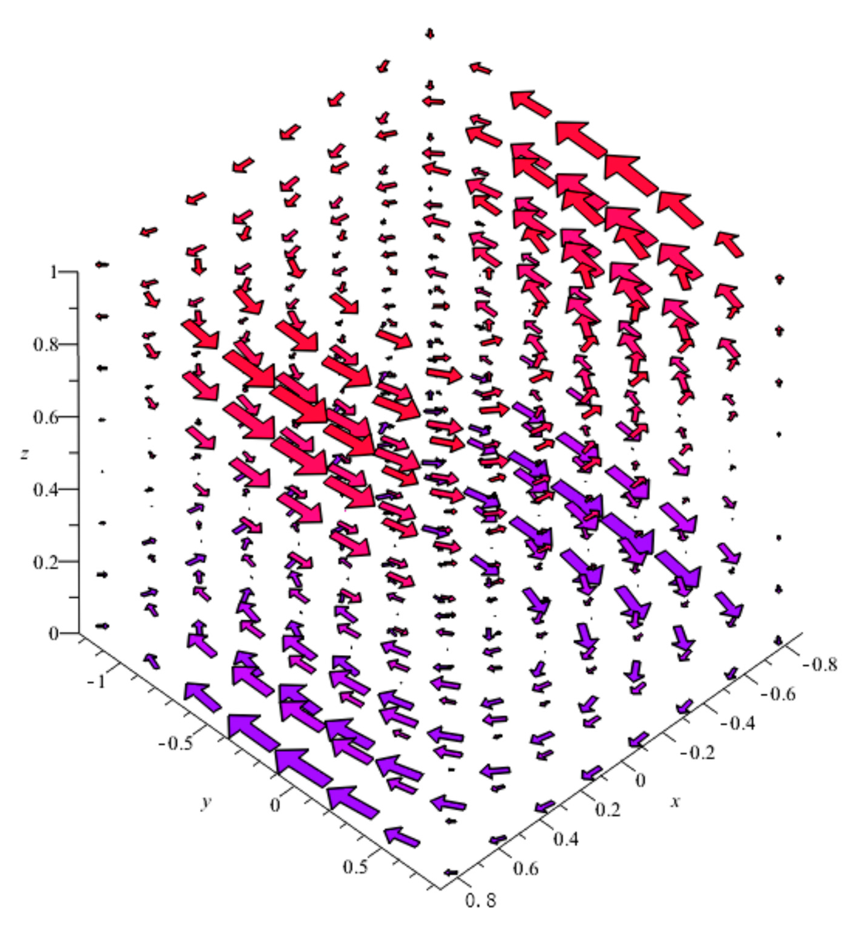
Figure 2.
The air parcel trajectory at nonzero divergence.
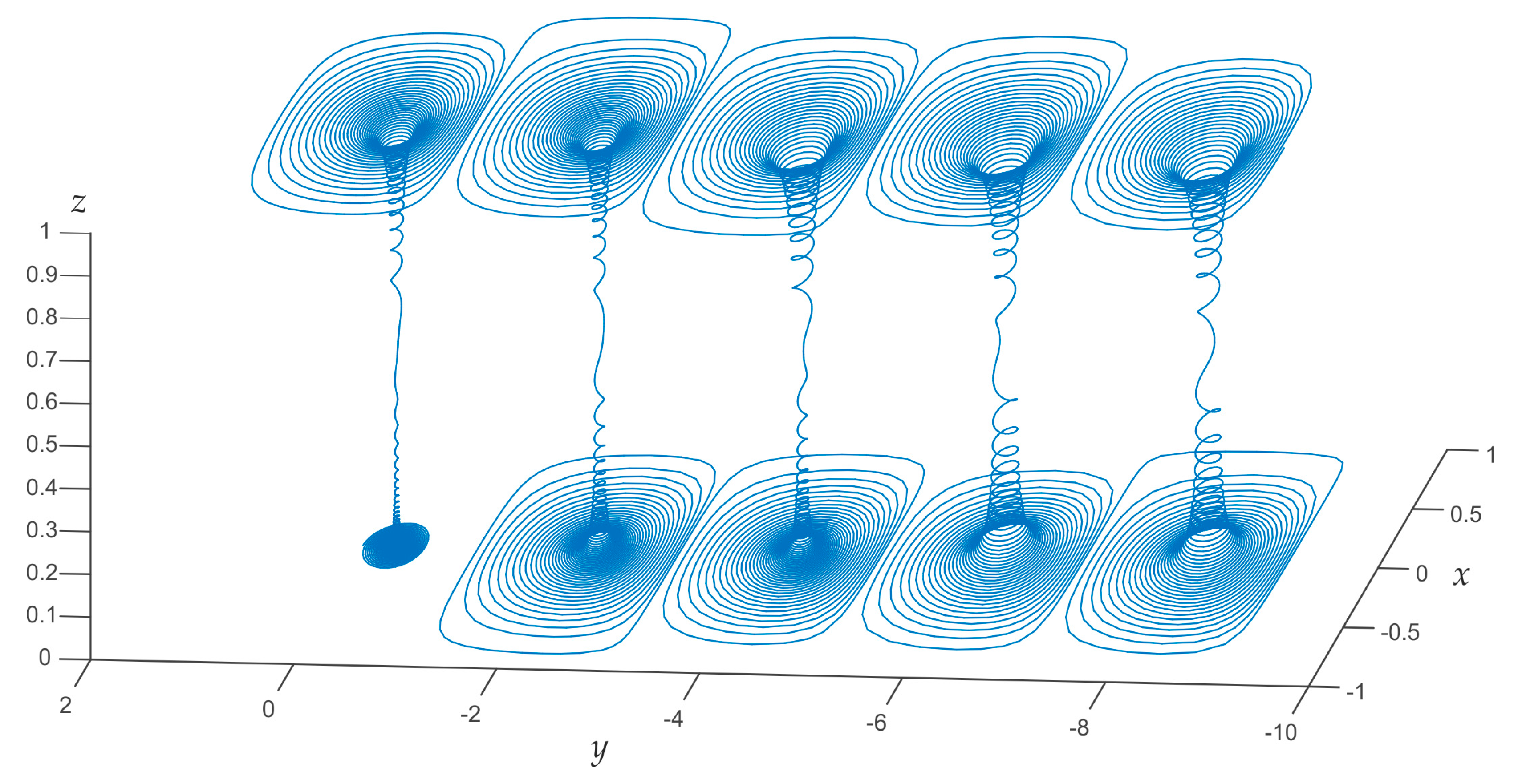
Figure 3.
The calculated fields of vorticity (a), temperature (b), divergence (c), and pressure (d) in lower part of the vortex cell (at ).
Figure 3.
The calculated fields of vorticity (a), temperature (b), divergence (c), and pressure (d) in lower part of the vortex cell (at ).

Figure 4.
The calculated fields of vorticity (a), temperature (b), divergence (c), and pressure (d) in upperpart of the vortex cell (at ).
Figure 4.
The calculated fields of vorticity (a), temperature (b), divergence (c), and pressure (d) in upperpart of the vortex cell (at ).

© 2018 by the authors. Licensee MDPI, Basel, Switzerland. This article is an open access article distributed under the terms and conditions of the Creative Commons Attribution (CC BY) license (http://creativecommons.org/licenses/by/4.0/).
Share and Cite
MDPI and ACS Style
Zakinyan, R.; Zakinyan, A.; Ryzhkov, R.; Semenova, J. Vortex Motion State of the Dry Atmosphere with Nonzero Velocity Divergence. Atmosphere 2018, 9, 61. https://doi.org/10.3390/atmos9020061
AMA Style
Zakinyan R, Zakinyan A, Ryzhkov R, Semenova J. Vortex Motion State of the Dry Atmosphere with Nonzero Velocity Divergence. Atmosphere. 2018; 9(2):61. https://doi.org/10.3390/atmos9020061
Chicago/Turabian StyleZakinyan, Robert, Arthur Zakinyan, Roman Ryzhkov, and Julia Semenova. 2018. "Vortex Motion State of the Dry Atmosphere with Nonzero Velocity Divergence" Atmosphere 9, no. 2: 61. https://doi.org/10.3390/atmos9020061
Note that from the first issue of 2016, this journal uses article numbers instead of page numbers. See further details here.