Ship-Based Measurements of Atmospheric Mercury Concentrations over the Baltic Sea

Department of Chemistry and Chemical Engineering, Chalmers University of Technology, Gothenburg 41258, Sweden
*
Author to whom correspondence should be addressed.
Atmosphere 2018, 9(2), 56; https://doi.org/10.3390/atmos9020056
Submission received: 24 November 2017
/
Revised: 19 January 2018
/
Accepted: 24 January 2018
/
Published: 9 February 2018
(This article belongs to the Special Issue Atmospheric Metal Pollution)
Abstract
:Mercury is a toxic pollutant emitted from both natural sources and through human activities. A global interest in atmospheric mercury has risen ever since the discovery of the Minamata disease in 1956. Properties of gaseous elemental mercury enable long range transport, which can cause pollution even in pristine environments. Gaseous elemental mercury (GEM) was measured from winter 2016 to spring 2017 over the Baltic Sea. A Tekran 2357A mercury analyser was installed aboard the research and icebreaking vessel Oden for the purpose of continuous measurements of gaseous mercury in ambient air. Measurements were performed during a campaign along the Swedish east coast and in the Bothnian Bay near Lulea during the icebreaking season. Data was evaluated from Gothenburg using plotting software, and back trajectories for air masses were calculated. The GEM average of 1.36 ± 0.054 ng/m3 during winter and 1.29 ± 0.140 ng/m3 during spring was calculated as well as a total average of 1.36 ± 0.16 ng/m3. Back trajectories showed a possible correlation of anthropogenic sources elevating the mercury background level in some areas. There were also indications of depleted air, i.e., air with lower concentrations than average, being transported from the Arctic to northern Sweden, resulting in a drop in GEM levels.
1. Introduction
Mercury is a toxic pollutant which is naturally abundant in the earth’s crust. It can be released to the atmosphere through volcanic and geothermal activities and the weathering of rocks. Emissions of mercury from anthropogenic sources come from mining, metal production, coal combustion, cement production and oil refining, among other sources [1]. The combustion of wood and refined petroleum products also releases mercury to the atmosphere [2]. Mercury is toxic in both inorganic and organic form. As methylated mercury, it is a neurotoxin and can damage a human’s central and peripheral nervous system [3,4]. Methyl-mercury (MeHg) poisoning, also called the Minamata disease, was officially discovered in 1956 in Minamata, Japan [5]. Because MeHg bioaccumulates in the aquatic food chain, humans consuming large amounts of fish and shellfish are thought to be at the highest risk for MeHg-poisoning [4,6].
Globally, one of the largest sources of anthropogenic mercury emissions to the atmosphere is presumed to be artisanal small-scale gold mining (ASGM) followed by coal combustion. However, exact values of ASGM emissions are hard to obtain due to an unregulated sector that may even be illegal in some cases [1]. In Sweden, the major mercury emission sources are combustion, the chemical industry on the west coast and metal and mining industries in northern Sweden [7]. Gaseous elemental mercury, also known as GEM or Hg0, is a very stable form of mercury and has a low deposition rate compared to Hg2+. GEM is the most abundant mercury species in the troposphere, having a residence time between 6 and 24 months [8,9]. An issue deriving from GEM’s stable nature is that it enables it to be transported on hemispheric scale and can therefore cause even pristine environments to be polluted [1,9].
While natural sources make up about 10% and anthropogenic sources make up about 30% of total Hg-emissions, the remaining part comes from re-emissions and is placed in a category of its own because the original source may have been either natural or anthropogenic. Once in the atmosphere, mercury circulates between air, earth and water. When mercury enters the ocean or freshwater, it has two possible paths other than being re-emitted. It can either be methylated by microorganisms and bio-accumulate in the food chain, or take the other path, which is the only way for the circulation to stop: it gets buried deep in bottom sediments or gets trapped in stable mineral compounds [1].
In the environment, mercury exists most commonly in oxidation states 0 or +II [10]. Oxidised mercury species are more soluble and can therefore easily fall down with precipitation and be deposited on vegetation and in oceans and fresh water [9,10,11]. Oxidation from GEM to gaseous oxidised mercury (GOM) is suggested to be caused by ozone, hydroxyl-radicals or halogens such as bromine. The sum of GEM and GOM is called total gaseous mercury (TGM). Since Hg0 has low solubility in water most aqueous mercury is therefore present in inorganic or organic form as Hg2+ or methylated mercury (MeHg) [10].
There are several studies that have found occasions in the polar regions where GEM is extensively oxidised into GOM or particulate mercury (HgP) in reactions with halogen radicals. The mechanism has yet to be confirmed but it is thought to involve halogen species that are released when open water areas refreeze and absorb UV-radiation [12]. These events are called atmospheric mercury depletion events (AMDE) and result in a sudden drop of GEM. They occur during springtime in Arctic and Antarctic regions, but there is evidence suggesting that mercury-depleted air masses may travel with the winds and be discoverable away from the polar areas [13].
1.1. Current State of Research
There has been extensive research on the subject of atmospheric mercury distribution ever since the discovery of the Minamata disease ([14,15,16] and references therein). The Minamata convention works toward protecting humans and the environment from mercury. It was agreed upon and adopted in 2013 and, as of August 2017, the Minamata convention has entered into force [17]. To understand the nature of mercury, how it travels and how it is transformed, it is important to map the concentrations at different locations around the world. A global observation network was created by the European Union, called the Global Mercury Observation System (GMOS), to support the Minamata convention and to facilitate the cooperation between countries. The GMOS programme collected data on mercury concentrations at different monitoring sites as well as during cruise campaigns. These data are used for research, such as the Mercury Air Transport and Fate Research run by the United Nations Environment Programme (UNEP) [18]. UNEP has also released several Global Mercury Assessments which present the latest research discoveries related to global emissions and distribution of mercury [1].
A previous study of mercury concentrations in and over the Baltic Sea was performed during the summer of 1997 and winter of 1998. Measurements were taken at various locations during two expeditions with results reflecting the normal background concentrations in winter but slightly higher during the summer expedition [19]. Continuous measurements have also been taken at Pallas, Finland which is close to the Baltic Sea [14]. Seasonal variations were observed by Kentisbeer et al. in a monitoring study in the United Kingdom in 2005–2008. The results showed a higher average concentration of mercury during the summer and could be explained by contaminated air masses coming with the southerly winds from continental Europe [20]. More commonly, winter and spring maxima have been found and are probably due to the increased burning of fossil fuels during the cold months [21,22,23]. In 1995 sudden drops in mercury levels were discovered during the spring at an Arctic monitoring site. Several other monitoring studies were able to confirm this phenomenon at other Polar regions. AMDE’s occur when GEM is oxidised into GOM or HgP resulting in a drop in TGM levels—these species are more reactive and therefore more likely to be transferred to the surroundings through reactions or deposition [12].
1.2. Aim and Conclusion
The aim of this study was to evaluate concentrations of GEM in ambient air in different parts of the Baltic Sea and to look for seasonal variations while comparing the results to other studies in the same and other areas. Reasons for varying GEM concentrations in different locations and the occurrence of AMDE’s during spring in Lulea was investigated. The collected data was compared and evaluated for seasonal variations of mercury levels in the air. It was found that, during the winter cruise, the average value was higher than the measured average value for the cruise south in late spring. Indications of depleted air coming from the Arctic were also discovered. The calculated average GEM levels were 1.365 ± 0.054 ng/m3 during winter and 1.288 ± 0.140 ng/m3 during spring with a total average of 1.362 ± 0.158 ng/m3.
2. Method
The Tekran model 2537A used for taking measurements was installed aboard the Swedish icebreaker vessel Oden (IB Oden) on the fourth deck, approximately 20 m above sea level. IB Oden, owned by the Swedish Maritime Administration, is not only an icebreaking vessel but also works as a platform for polar research and has thus far made seven research expeditions to the North Pole and worked six seasons in Antarctica. IB Oden being a research vessel was made possible by a contract between the Swedish Maritime Administration and the Swedish Polar Research Secretariat, which is another government-ruled organisation focusing on promoting polar research [24].
Continuous GEM measurements in ambient air above the surface of the Baltic Sea were conducted during a campaign aboard IB Oden. The Baltic Sea is a young sea with brackish water which makes it a challenging environment for organisms to inhabit. The environmental conditions have become increasingly harmful due to heavy pollution and eutrophication from the many residential areas on the coastlines [25]. The geographical location of the Baltic Sea in the northern latitudes results in great variations in temperature and hours of daylight during different seasons. The proximity to the Arctic also makes it possible for AMDEs to travel south with the winds and be discoverable in this area [13]. Some of the northernmost parts—such as the Bothnian Bay—are covered in ice during winter thus there is a need for icebreaking vessels to ensure that freight ships have access to the most important harbours. The duration of the icebreaking season varies each year, and so every year from November to May the Swedish Meteorological and Hydrological Institute (SMHI) maps the ice around and along Sweden’s coasts [26].
Oden travelled from Helsingborg to Lulea in December 2016 and returned back south (to Landskrona this time) in May 2017. During the months in between, Oden was breaking ice in the Bothnian Bay while Tekran was still performing continuous measurements. The cruise north from Helsingborg to Lulea (North Cruise) took place between 2 and 6 December. The icebreaking season in the Bothnian Bay (BB) was divided into three groups due to a large amount of data—they will be referred to as BB1, BB2 and BB3. The first measurements from the icebreaking season were conducted in March 2017—the specific dates can be found in Table 1. Oden returned back from Lulea to Landskrona (South Cruise) between 28 April and 5 May. A map showing some key locations can be seen in Figure 1.
2.1. Mercury Analyser
A Tekran 2537A was stationed at the bow of IB Oden and used for all the measurements of GEM. Continuous measurements was made with ten minutes resolution. Tekran utilises cold vapour atomic fluorescence spectroscopy (CV-AFS),) for determining mercury concentrations in the air. The air inlet was placed at the same level as Tekran at 20 m in a direction opposite of the ship’s funnel, to avoid getting exhaust gas in the inlet. If a sudden spike in GEM levels appeared in the measured data, wind direction in combination with the direction of the ship was studied to see if the wind might have blown exhaust gas in the direction of the air inlet. The wind speed was also studied because low wind speed at a high measurement point indicates contamination from exhaust gases.
The detection compartment of the instrument consists of a hollow-cathode lamp, emitting light at 253.7 lambda which is mercury’s absorbance line, as well as a photomultiplier tube. According to the Tekran manufacturers the detection limit of Tekran 2537A is 0.1 ng/m3 [27,28].
As Tekran 2357A operated almost completely unattended during this study, the input method was set to auto-calibration at a 24 h interval via the internal permeation source to control the data quality. Before calibration, the system and gold traps are cleansed with Argon gas to remove any mercury still in the system. Then, zero air is purged through the system before the calibration starts. Air was collected from the room where the Tekran instrument was installed and cleansed to zero air when passing through a carbon filter. The permeation source is a built in mercury source from which a known amount is extracted for each calibration [28]. Calibration can also be managed manually. The calibration works the same way as the auto-calibration calibrating the system using the internal permeation source with the difference that manual calibrations can be forced onto the system.
The sampling flow rate was 1 L/min and the sampling interval on each cartridge was 10 min. As air enters the inlet and is carried towards the instrument, it passes a soda-lime trap which scrubs the incoming air from unwanted substances such as hydrocarbons, dirt and moist. Thereafter, it also passes a Teflon-filter (Polytetrafluoroethylene (PTFE) filter), which in turn filters out HgP from entering the system. It is also presumed that this filter collected all GOM from the samples. By using two gold traps, continuous measurements are enabled. Inside the cartridges, the mercury is trapped by the amalgamation technique and adsorbed onto the gold. The gold trap is then heated and GEM is desorbed to the detector. Argon gas carries the gaseous elemental mercury at a flow rate of approximately 80 mL/min to the detector. In between measurements, the flow rate of Argon is about 5 mL/min. As one trap samples air, the other is heated and desorbed to the detector, and then they switch tasks [28].
During this study, calibrations were performed manually using the Tekran internal calibration source on the following occasions: namely 2 December, which was the first day of this study’s measurements, and on 10 March. The last calibration was performed on 23 March. Few calibrations and relatively long intervals between calibrations may cause uncertainties in the measurements. However, the calibrations looked satisfactory in terms of showing similar areas. Furthermore, the data and the standard deviation were not unusual in comparison to the background level of TGM in the northern hemisphere.
A comparison between calibration data from this study and from a previous measurement campaign during summer 2016 using the same instrument and the same internal hollow-cathode lamp was performed to determine how much the lamp possibly could have aged between calibrations. By comparing the area responses from different calibrations, an indication of the lamp’s degradation is obtained. Calibration data from the summer campaign indicated that there was no major change in response [10]. However, on 10 March 2017 a new hollow-cathode lamp was installed inside the instrument and between the calibrations on the 10 March and on the 23 March a 23% decline in area response was calculated and corrected for.
2.2. Softwares
The ocean data view (ODV) program, version 4.7.10, was used for plotting and analysing data [29]. In this study the ship coordinates were combined with the Tekran data to visualise the concentrations along the ship’s track [30]. Other parameters such as wind speed and wind direction were plotted to indicate whether they influenced the fluctuating concentrations. The National Oceanic and Atmospheric Administration’s hybrid single-particle Lagrangian integrated trajectory (NOAA HYSPLIT) online trajectory model was used to produce back trajectories of air masses [31]. The setup used for HYSPLIT was Global Data Assimilation System (GDAS) 1°, global, 2006–present. In this study, HYSPLIT was used to calculate back trajectories to see where air masses originated from before they reached the coordinate of interest. These calculations were used as an aid to find possible explanations as to why an area had lower or higher concentrations than the average background mercury levels. Four day backward trajectories of air masses were produced at three different vertical levels (0, 20 and 100 m), for the coordinate interest. HYSPLIT was also used to look at solar flux, precipitation, temperature and humidity [32].
3. Results and Discussion
Continuous measurements of GEM were carried out during the North Cruise from Helsingborg to Lulea, during icebreaking season in the Bothnian Bay and during the South Cruise from Lulea to Landskrona. The average concentrations are presented in Table 1, divided into five intervals according to location and time. An average of all the collected data was calculated as well. The measured average values were comparable to normal background concentrations of TGM in the northern hemisphere which is approximately 1.5–1.7 ng/m3 [20]. Most of the data, however, show lower values, particularly the measurements from BB1. Standard deviations were also calculated to view differences and fluctuations in our measurements.
3.1. Anthropogenic Sources
When evaluating the data and looking at back trajectories for low or elevated concentrations, possible anthropogenic emission sources for elevated levels were searched for. Air masses that had passed through northern parts of Sweden often resulted in elevated levels. In 2016, one county located in the most northern part of Sweden was the largest contributor of mercury emissions to the air, followed by south-eastern and south-western counties. In northern Sweden, the mining and metal industries are the predominant atmospheric mercury emission sources, and in mid- and southern Sweden, the combustion and chemical industries are the main sources of atmospheric mercury. However, there seems to be a declining trend in the overall anthropogenic mercury emissions to the atmosphere in Sweden when comparing emission data sheets from the last ten years [7]. On a few occasions, back trajectories showed winds that had passed through areas in Finland where there are gold mines and also a known chlor-alkali factory [33,34]. These are also mercury emission sources that have possibly impacted the elevated levels observed in this study.
3.2. Observations from the Plots
Each cruise was plotted on a map using ODV software. Coordinates of significantly high or low concentrations were investigated by calculating back trajectories. The most important events are presented in Section 3.2.1, Section 3.2.2 and Section 3.2.3 and possible anthropogenic sources are discussed.
3.2.1. Cruise North
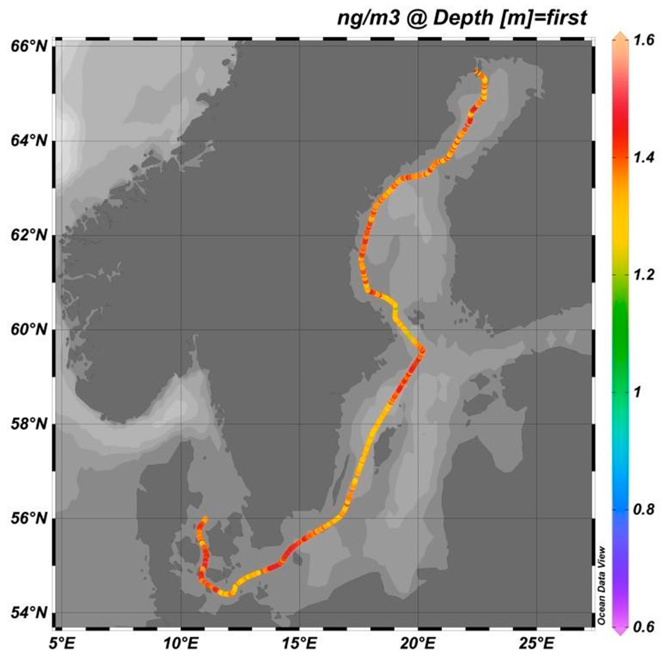
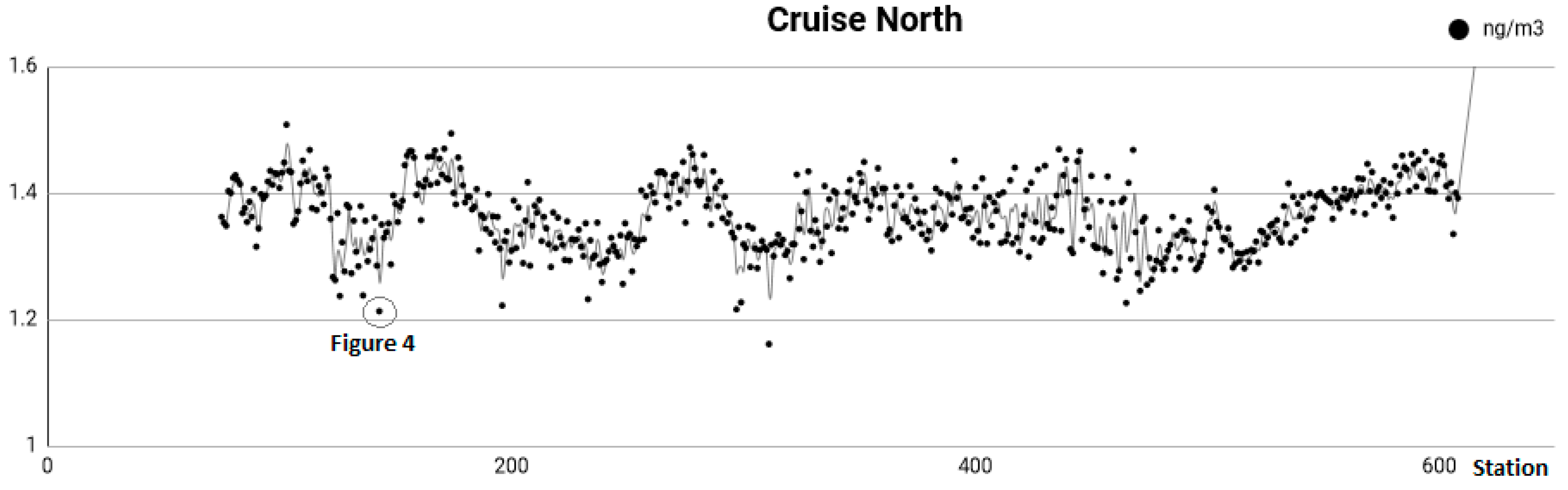
On the cruise north from Helsingborg to Lulea the measured average concentration reflected normal background levels. There were areas with higher GEM levels near the Danish islands, south of Sweden and Stockholm (see Figure 2). For these events it was expected that the winds would originate in more populated areas such as the nearby urban areas or continental Europe. However, back trajectories showed consistent northerly winds for most of the cruise. There was no exceptionally high value measured and even the slightly higher values did not deviate far from normal background levels. A graph presenting all measured values during the cruise north can be seen in Figure 3.
As can be seen in Figure 2, Oden’s transit north appears to start between the Danish Islands. One reason for this is that the measurements in Helsingborg, and a few hours after Oden left port, were unreasonably low and thus excluded from the results. The other reason was a blackout that occurred on the 2 December shortly after IB Oden left port in Helsingborg. When online again it was decided to calibrate Tekran and after the calibration was performed the data appeared normal.
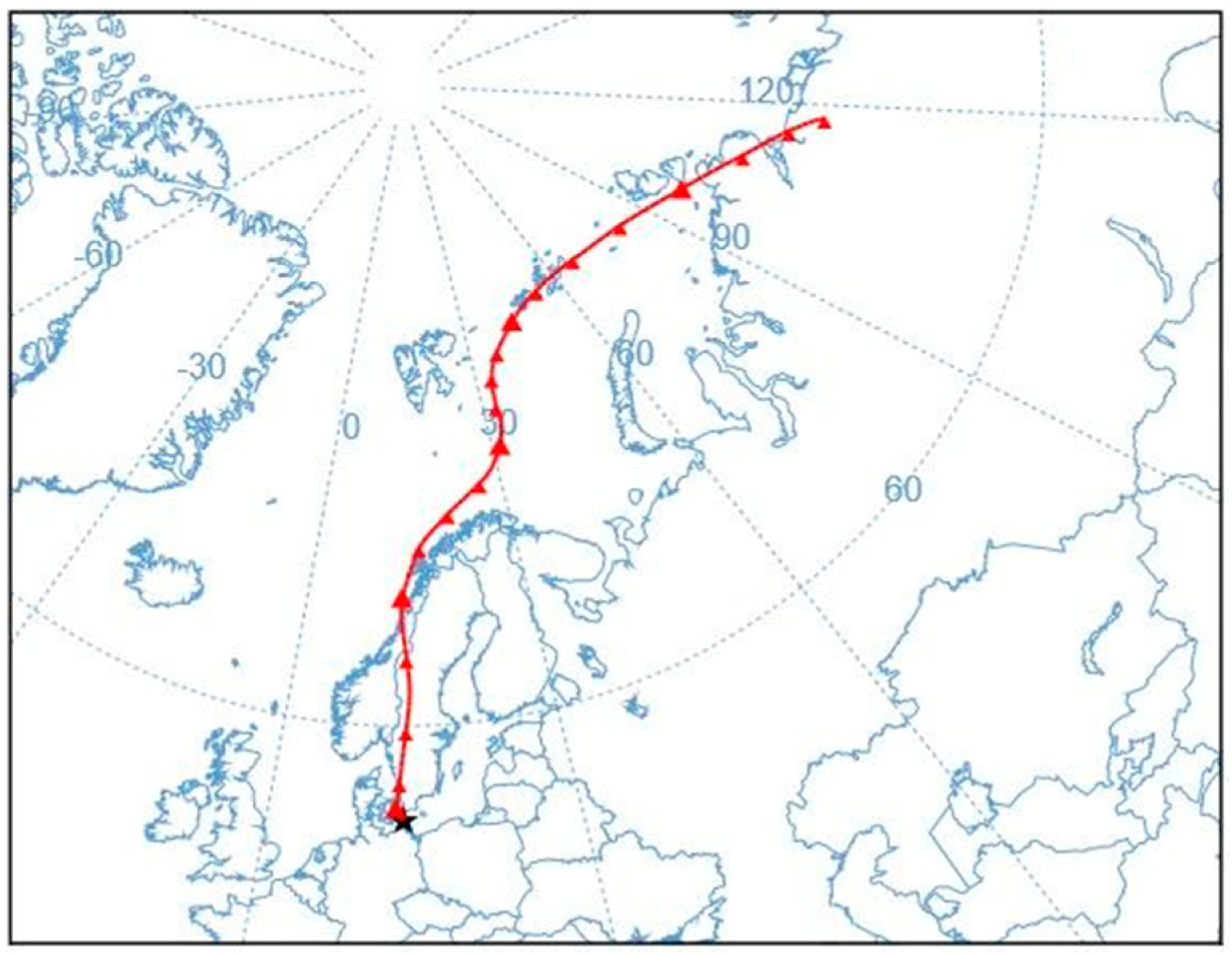
The somewhat elevated GEM levels near the Danish islands were investigated. Back trajectories showed northern winds passing through Denmark, Norway and in some cases all the way from Iceland, before reaching Oden. A low point was also investigated (see Figure 4) and showed similar trajectory patterns with winds coming from the north. However, for some elevated levels where the winds had passed over the North Sea, no specific source of emission was found. Perhaps wood combustion from the mainland could be the reason, or fumes from passing ships or sudden changes in the wind that carried fumes from Oden’s own exhaust pipe. Furthermore, the source of emission could be located so far away that it did not show up on the four-day trajectories.
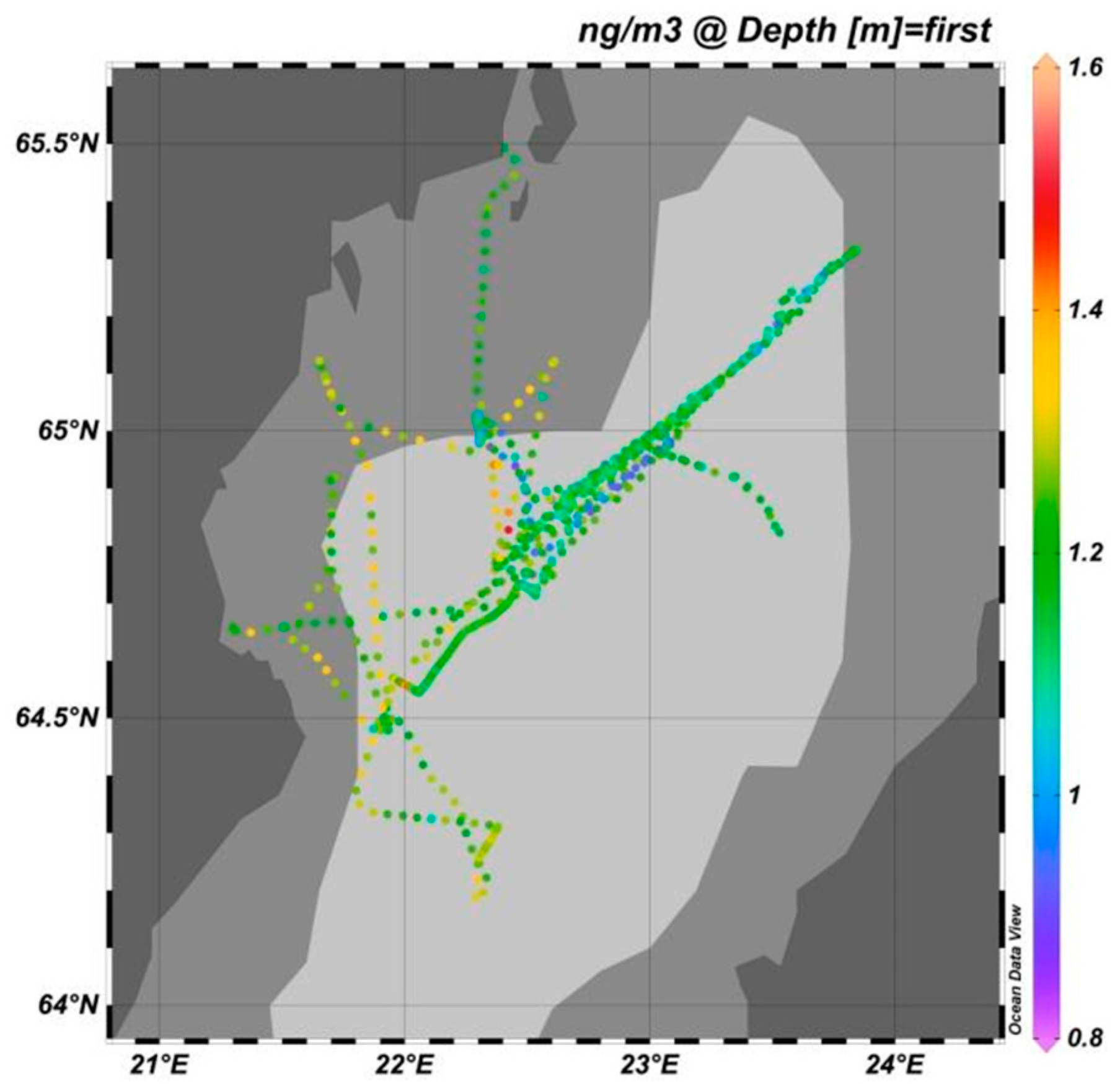
In the northern parts of Sweden, there were generally higher GEM levels compared to southern part (see Figure 1). Using HYSPLIT to investigate some high level coordinates, winds were observed to have passed through Finland before reaching Sweden. In Figure 5, back trajectory winds pass over areas in Finland where there are both gold mines and chemical industry emitting mercury to the air [33,34]. Contaminated air from these anthropogenic sources is a possible reason as to why there were areas of elevated GEM levels seen in the plot. Winds reaching the areas of lower concentrations can be assumed to have bypassed these sources but it is difficult to see the exact trajectory path in the HYSPLIT diagrams.
3.2.2. Bothnian Bay
Data was also collected during icebreaking season in the Bothnian Bay and were divided into three separate groups: BB1, BB2 and BB3. Plots are presented for BB1 (Figure 6) and BB2 (Figure 7) but not for BB3 as the vessel was stationed at port in Lulea for this time period. The lowest average GEM was calculated for the BB1 icebreaking cruise. At first, a calibration error was suspected. Because of this, the calibration on 10 March was examined carefully, but it seemed to be in order. Back trajectories of air masses did not correlate with the levels of GEM measured. In some cases, there were low concentrations, with winds passing by known anthropogenic sources of atmospheric mercury. In other cases this was reversed. Three graphs presenting all measured values during BB1, BB2 and BB3 can be seen in Figure 8, Figure 9 and Figure 10.
During the icebreaking season and BB2, the highest mercury level of 2.675 ng/m3 was measured. One explanation is possible contamination from the ship’s exhaust since it greatly differs from the other measured values. A supporting argument for this case is that the wind speed was unusually low at this particular measurement. This was also true for all the occasions where the mercury level approached 2.0 ng/m3 during BB2. The average value for BB2 was higher than for all the other groups, especially high values were measured during the last week of March. On average, the wind speeds were lower during BB2 than during the other cruises, which could be an explanation for the high mercury levels. Towards the end of this cruise, the values seem to drop towards more normal background levels.
During the evaluation of data from Bothnian Bay, two possible AMDEs were discovered on 28 March and 18 April. The first was found on BB2, where a dip in the concentrations was observed with the lowest measured value at 1.100 ng/m3 found on 28 March. Back trajectory showed winds coming from the Arctic, possibly carrying depleted air to the Bothnian Bay. The other possible indication of an AMDE was found on 18 April, when the ship was stationed in the Lulea harbour. The concentration dropped suddenly to 0.817 ng/m3 and, as can be seen in Figure 11, back trajectories showed that winds originated in the Arctic, passing through Svalbard. Since the winds did not pass through any apparent anthropogenic mercury sources this suggests a potential AMDE.
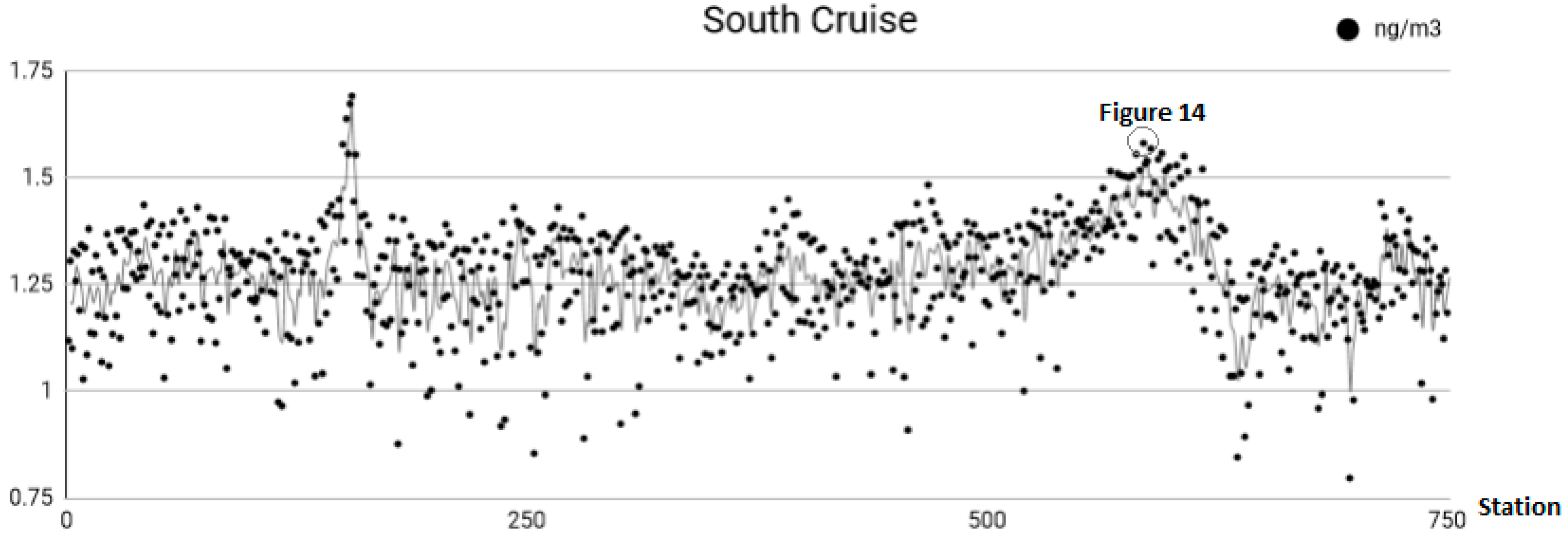
3.2.3. Cruise South
On the cruise south to Landskrona, the measurements were comparable to normal background concentrations. The calculated average was lower compared to the winter average. There was missing or faulty ship location data causing a few gaps in the ODV-plot for the cruise south (see Figure 12). This is because of a problem with the ship’s coordinate data storing but it did not affect the calculation of the average concentration. A graph presenting all measured values during the cruise south can be seen in Figure 13.
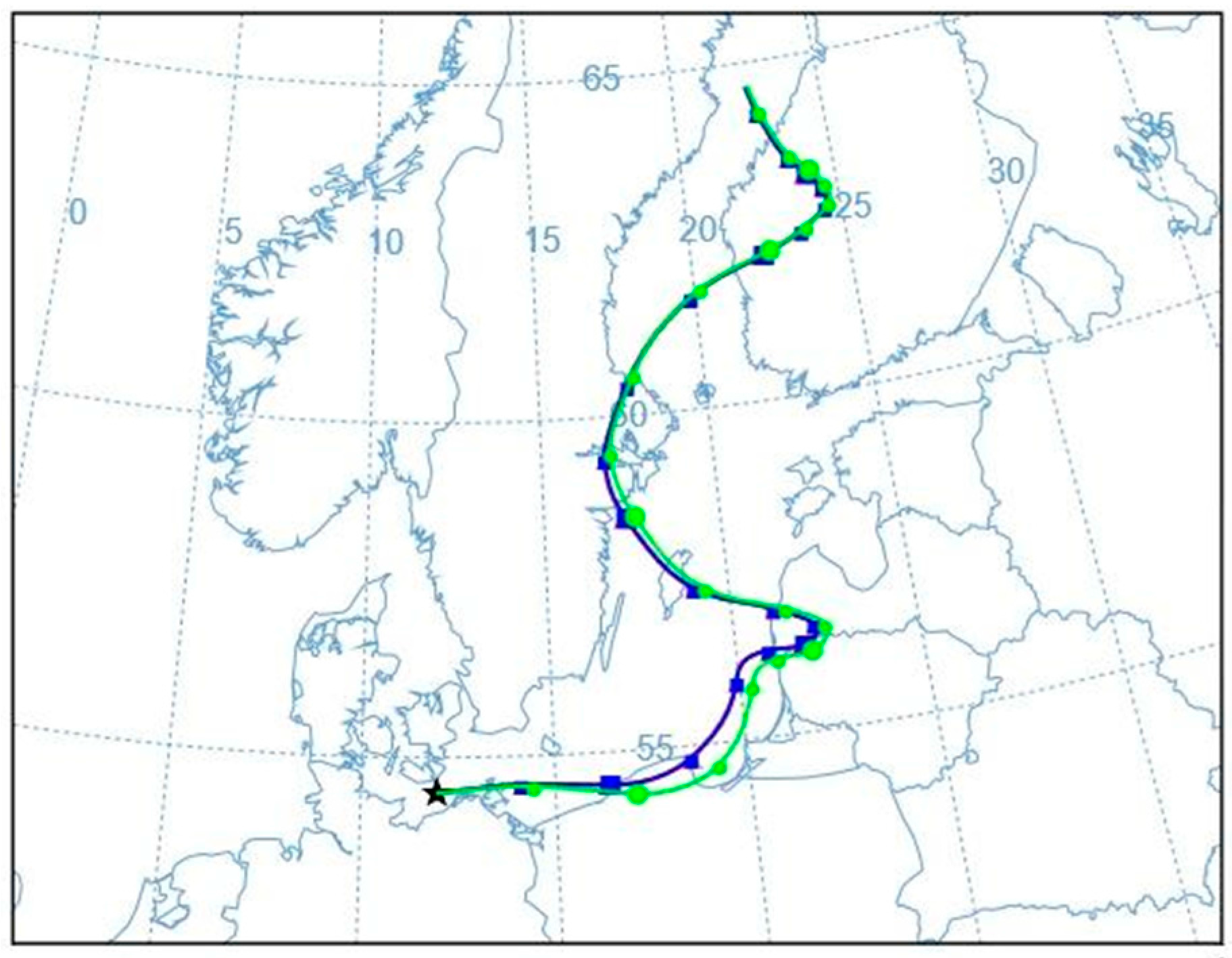
Elevated levels of GEM were measured in the Gulf of Bothnia, near Ornskoldsvik in Sweden. According to back trajectories the winds passed through or near gold mines and chemical industry in western and northern Finland, possibly carrying mercury-rich air and causing higher GEM levels in this area [33,34]. Another occasion where the concentrations were greater than the average was found between Denmark and Germany. Back trajectories showed winds coming from the east passing through Stockholm, Latvia and Lithuania and then passing by the coast of Poland and Germany (see Figure 14). As these countries have higher mercury emissions compared to the Nordic countries it was expected to find higher levels of GEM with eastern winds [35].
3.3. Comparisons and Other Observations
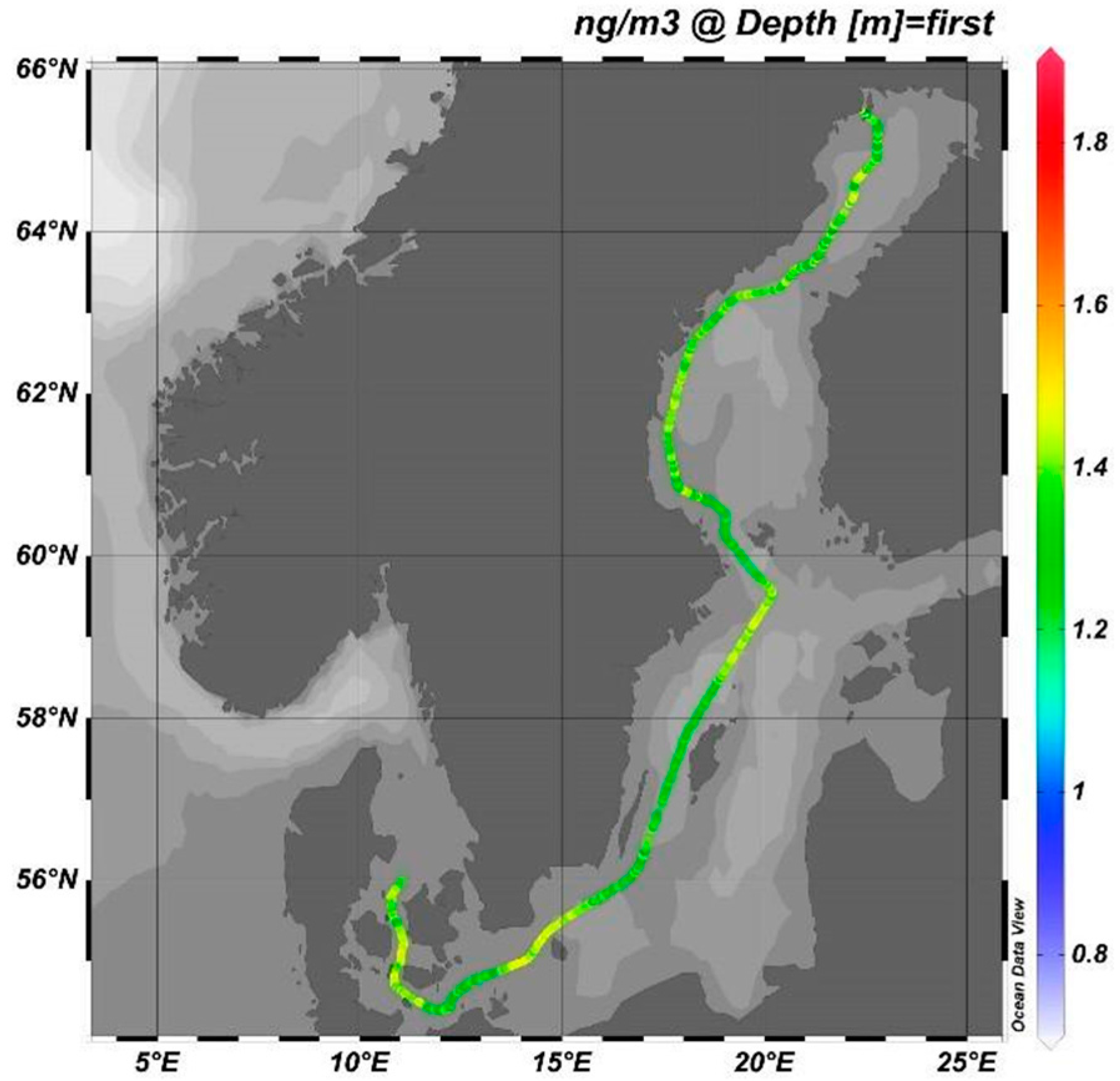
Comparing Figure 15 and Figure 16, depicting the cruise to northern Sweden during winter and the cruise to southern Sweden during spring, it can be seen that, during winter, the GEM concentrations are higher. However, while the average for the North Cruise was higher than the average for the South Cruise, the standard deviation for the South Cruise was higher. This indicates that the difference in the winter and the summer averages cannot be discriminated between. Measurements conducted over a longer time period would be needed to safely evaluate if seasonal trends are occurring in the Baltic Sea. Such studies have been performed in the northern hemisphere and winter or spring maxima have been found [21,22,23].
It is believed that higher mercury levels during winter are caused by the increased burning of fossil fuels for domestic heating in the winter. Another possible explanation for this trend is that a higher abundance of atmospheric oxidants in summer causes Hg to oxidise and deposit onto surfaces, resulting in decreased TGM levels [21,36]. The opposite trend—a summer maximum—has also been observed in the United Kingdom and in the Baltic [19,20]. This is probably due to a larger influence of southerly winds carrying contaminated air from continental Europe [20]. Kuss et al. has found that the Baltic Sea can act as a sink for mercury during winter season. The uptake of elemental mercury by the surface water is dependent on the concentration of GEM in air, the concentration of dissolved gaseous elemental mercury (DGM) in the surface water [37,38,39]. Moreover, mathematical modelling of air sea exchange also includes e.g., water temperature and wind speed. Since measurements of DGM in the surface water or sea-ice were not performed in this project, the importance of sea water as a sink, or source, for GEM cannot be estimated during the seasons investigated.
On average, the GEM levels for both cruises are similar to what earlier studies of background TGM levels have found, with some exceptions of elevated TGM levels in certain areas (see Table 2). On both transits, north and south, mercury concentrations were elevated near the Danish Islands. For the north cruise no obvious anthropogenic sources were found to be the cause. On one occasion, air masses passed through the Swedish west coast near known mercury emission sources. Conversely, during other occasions, air masses passed through Denmark, Norway and Iceland where no specific sources were found. On the cruise south during spring the elevated levels were most likely caused by atmospheric mercury being transported from continental Europe and the Baltic, as previously mentioned.
Air mass trajectories originating in mercury rich areas mostly correlated with elevated measurements. However, there were instances where back trajectories did not always give a clear answer as to why a certain measurement was either elevated or not. In several cases of elevated levels air masses passed through areas where no known source of emission could be found. The reverse was also observed for some low measurements.
A declining trend has been observed for the last 10–30 years in sub-Arctic and mid-latitude sites [8,22,43,44]. This trend is corroborated by comparing the measured values in this study with measurements from previous studies. Measurements were performed in Hoburg on the Swedish east coast as early as in 1979–1980 resulting in an average of 3.91 ng/m3 which is nearly 300% higher than the average from this study [23]. A later study was performed in 1997–1998 where measurements were taken at various locations over the Baltic Sea. During summer in 1997 an average of 1.70 ng/m3 was found which is about 30% higher than the south cruise average of this study. During winter 1998 the calculated average was 1.38 ng/m3 which does not differ significantly from the winter average of this study [19].
During the cruise north, a diurnal variation pattern was observed, with elevated levels during the day and lower levels at night. This pattern was not consistent once IB Oden had passed Stockholm, nor was it observed again on the other cruises.
4. Conclusions
Data was evaluated with the aid of the programs ODV and HYSPLIT. Average concentrations, for the transits north and south as well as during the icebreaking season, were 1.365 ng/m3 (north), 1.288 ng/m3 (south), 1.164 (BB1), 1.509 ng/m3 (BB2) and 1.364 ng/m3 (BB3). The total average was 1.362 ng/m3. When IB Oden was heading north during the winter, the average value was found to be higher than the measured average value for the cruise south in late spring. However, the difference between the average values was not statistically significant. Collecting data over a longer time period would be needed in order to determine if there is a seasonal trend. Over the past 10–30 years a declining trend in atmospheric mercury concentrations has been observed [8,22,43]. When comparing the average values of this study with measurements from previous studies made in the Baltic, this observation was supported.
Elevated levels were found near the Danish islands during both winter and spring. In winter, there were elevated levels near and above Stockholm and during the spring cruise an area of high levels was found near Ornskoldsvik, Sweden. Using HYSPLIT to calculate air mass trajectories, some winds were observed to have passed through places of known mercury sources such as continental Europe or mining and metal companies in Sweden and Finland. However, during other occasions of elevated levels, back trajectories did not give sufficient indications of possible anthropogenic sources. In many of these cases, the winds had instead travelled over the North Sea, indicating that the elevated levels were possibly caused by unknown sources on the mainland of northern and middle Sweden. Other possible reasons include winds that may have passed through fumes of passing ships or Oden’s own exhaust pipe. However, because of GEM’s stable nature, it can be difficult to pinpoint the exact emission source—if it is far away, the four-day trajectory may not have been long enough. Low or lower values compared to normal background levels were also of interest when calculating back trajectories as particularly low values could be indications of AMDEs. On two occasions during spring, the levels clearly dropped while oncoming winds came from the Arctic region. This result suggests that depleted air masses had reached the site of measurement.
Supplementary Materials
The supplementary file is available on https://www.mdpi.com/2073-4433/9/2/56/s1.
Acknowledgements
The Swedish Polar Research Secretariat and Captain and crew onboard IB Oden are acknowledged for support.
Author Contributions
H. Hoglind and S. Eriksson have analysed all data, made the Hysplit simulations and also been the main authors of the manuscript. K. Gardfeldt has planned the measurement campaign, installed the Tekran 2537A onboard the IB Oden and been the co-author of the manuscript.
Conflicts of Interest
The authors declare no conflict of interest.
References
- UNEP. Global Mercury Assessment 2013: Sources, Releases and Environmental Transport; UNEP Chemicals Branch: Geneva, Switzerland, 2013. [Google Scholar]
- Sunderland, E.M.; Chmura, G.L. The history of mercury emissions from fuel combustion in Maritime Canada. Environ. Pollut. 2000, 110, 297–306. [Google Scholar] [CrossRef]
- Pirrone, N.; Mahaffey, K.R. Where we stand on mercury pollutution and its health effects on regional and global scales. I. In Dynamics of Mercury Pollution on Regional and Global Scales: Atmospheric Processes and Human Exposures around the World; Pirrone, N., Mahaffey, K.R., Eds.; Springer Science, Buisness Media Inc.: New York, NY, USA, 2005. [Google Scholar]
- World Health Organization. Mercury and Health; World Health Organization: Geneva, Switzerland, 2017; Available online: http://www.who.int/mediacentre/factsheets/fs361/en/ (accessed on 24 November 2017).
- Harada, M. Minamata Disease: Methylmercury Poisoning in Japan Caused by Environmental Pollution. Crit. Rev. Toxicol. 2008, 25, 1–24. [Google Scholar] [CrossRef] [PubMed]
- Tekran Instruments Corporation. Mercury Science. Mercury in the Environment; Tekran Instruments Corporation: Toronto, ON, Canada, 2017; Available online: http://www.tekran.com/mercury-science/mercury-in-the-environment/ (accessed on 24 November 2017).
- Naturvårdsverket. Utsläpp i Siffror. 2016. Available online: http://utslappisiffror.naturvardsverket.se/ (accessed on 24 November 2017).
- Cole, A.S.; Steffen, A.; Pfaffhuber, K.A.; Berg, T.; Pilote, M.; Poissant, L.; Tordon, R.; Hung, H. Ten-year trends of atmospheric mercury in the high Arctic compared to Canadian sub-Arctic and mid-latitude sites. Atmos. Chem. Phys. 2013, 13, 1535–1545. [Google Scholar] [CrossRef] [Green Version]
- Fu, X.W.; Feng, X.; Dong, Z.Q.; Yin, R.S.; Wang, J.X.; Yang, Z.R.; Zhang, H. Atmospheric gaseous elemental mercury (GEM) concentrations and mercury depositions at a high-altitude mountain peak in south China. Atmos. Chem. Phys. 2010, 10, 2425–2437. [Google Scholar] [CrossRef]
- Nerentorp, M. Mercury Cycling in the Global Marine Environment. Ph.D. Thesis, Chalmers University of Technology, Gothenburg, Sweden, 2016. [Google Scholar]
- Gårdfeldt, K. Kvicksilver Från Havet. 2001. Available online: https://www.havet.nu/dokument/HU20012kvicksilver.pdf (accessed on 24 November 2017).
- Steffen, A.; Douglas, T.; Amyot, M.; Ariya, P.; Aspmo, K.; Berg, T.; Bottenheim, J.; Brooks, S.; Cobbett, F.; Dastoor, A.; et al. A synthesis of atmospheric mercury depletion event chemistry in the atmosphere and snow. Atmos. Chem. Phys. 2008, 8, 1445–1482. [Google Scholar] [CrossRef] [Green Version]
- Nerentorp, M.; Kyllonen, K.; Wängberg, I.; Kuronen, P. Speciation measurements of airborne mercury species in northern Finland; Evidence for long range transport of air masses depleted in mercury. In Proceedings of the 16th International Conference on Heavy Metals in the Environment, Rome, Italy, 23–27 September 2012; EDP Sciences: Paris, France, 2013. [Google Scholar]
- Sprovieri, F.; Pirrone, N.; Bencardino, M.; D’Amore, F.; Carbone, F.; Cinnirella, S.; Mannarino, V.; Landis, M.; Ebinghaus, R.; Weigelt, A.; et al. Atmospheric mercury concentrations observed at ground-based monitoring sites globally distributed in the framework of the GMOS network. Atmos. Chem. Phys. 2016, 10, 11915–11935. [Google Scholar] [CrossRef]
- Angot, H.; Dastoor, A.; Simone, F.; Gårdfeldt, K.; Gencarelli, C.N.; Hedgecock, I.M.; Langer, S.; Magand, O.; Mastromonaco, M.N.; Nordstrøm, C.; et al. Chemical cycling and deposition of atmospheric mercury in polar regions: Review of recent measurements and comparison with models. Atmos. Chem. Phys. 2016, 16, 10735–10763. [Google Scholar] [CrossRef] [Green Version]
- Sprovieri, F.; Pirrone, N.; Ebinghaus, R.; Kock, H.; Dommergue, A. A review of worldwide atmospheric mercury measurements. Atmos. Chem. Phys. 2010, 10, 8245–8265. [Google Scholar] [CrossRef] [Green Version]
- United Nations Environment. Convention; United Nations Environment: Geneva, Switzerland, 2017; Available online: http://www.mercuryconvention.org/Convention/tabid/3426/language/en-US/Default.aspx (accessed on 24 November 2017).
- Global Mercury Observation System. Available online: http://www.gmos.eu/index.php/groud-based (accessed on 24 November 2017).
- Wängberg, I.; Schmolke, S.; Schager, P.; Munthe, J.; Ebinghaus, R.; Iverfeldt, Å. Estimates of air-sea exchange of mercury in the Baltic Sea. Atmos. Environ. 2001, 35, 5477–5484. [Google Scholar] [CrossRef]
- Kentisbeer, J.; Leaver, D.; Cape, J.N. An analysis of total gaseous mercury (TGM) concentrations across the UK from a rural sampling network. J. Environ. Monit. 2011, 13, 1653–1661. [Google Scholar] [CrossRef] [PubMed] [Green Version]
- Ebinghaus, R.; Kock, H.H.; Coggins, A.M.; Spain, T.G.; Jennings, S.G.; Temme, C. Long-term measurements of atmospheric mercury at Mace Head, Irish west coast, between 1995 and 2001. Atmos. Environ. 2002, 36, 5267–5276. [Google Scholar] [CrossRef]
- Slemr, F. Trends in atmospheric mercury concentrations over the Atlantic Ocean and the Wank summit and the resulting constraints on the budget of atmospheric mercury. I. In Global and Regional Mercury Cycles: Sources, Fluxes and Mass Balances; NATO ASI Series; Baeyens, W., Ebinghaus, R., Vasiliev, O., Eds.; Kluwer: Dordrecht, The Netherlands, 1996; pp. 33–84. [Google Scholar]
- Brosset, C. Total airborne mercury and its possible origin. In Water, Soil and Air Pollution; Springer: Berlin/Heidelberg, Germany, 1982; Volume 17, pp. 37–50. [Google Scholar]
- Swedish Maritime Administration. Isbrytaren/Forskningsfartyget Oden; Swedish Maritime Administration: Norrköping, Sweden, 2016. Available online: http://sjofartsverket.se/oden (accessed on 24 November 2017).
- Fonselius, S.; Eklund, R.; Warell, J.; Strömberg, J.O. Östersjön. I: NE Nationalencyklopedin. Malmö. Available online: http://www.ne.se/uppslagsverk/encyklopedi/l%C3%A5ng/%C3%B6stersj%C3%B6n (accessed on 24 November 2017).
- Swedish Meteorological and Hydrological Insitute. Havsis; Swedish Meteorological and Hydrological Insitute: Norrköping, Sweden, 2018. Available online: http://www.smhi.se/klimatdata/oceanografi/havsis (accessed on 24 November 2017).
- Tekran Instruments Corporation. The NEW Tekran® 2537X Automated Ambient Air Analyzer; Tekran Instruments Corporation: Toronto, ON, Canada, 2018; Available online: http://www.tekran.com/products/ambientair/tekran-model-2537-cvafs-automated-mercury-analyzer/ (accessed on 24 November 2017).
- Tekran Instruments Corporation. Tekran Manual: Model 2537A Mercury Vapour Analyzer User Manual; Tekran Instruments Corporation: Toronto, ON, Canada, 1997. [Google Scholar]
- Schlitzer, R. Ocean Data View. 2017. Available online: http://odv.awi.de (accessed on 24 November 2017).
- Ocean Data View Homepage. Bremerhaven: Alfred Wegener Institute for Polar and Marine Research. 2017. Available online: https://odv.awi.de/ (accessed on 24 November 2017).
- Rolph, G.; Stein, A.; Stunder, B. Real-time Environmental Applications and Display System: READY. Environ. Model. Softw. 2017, 95, 210–228. [Google Scholar] [CrossRef]
- Description. National Oceanic and Atmospheric Administration Air Resources Laboratory: College Park, MD, USA, 2016. Available online: http://www.arl.noaa.gov/HYSPLIT_info.php (accessed on 24 November 2017).
- The Geological Survey of Finland. Metals and Minerals Production; The Geological Survey of Finland: Espoo, Finland, 2016; Available online: http://en.gtk.fi/informationservices/mineralproduction/ (accessed on 24 November 2017).
- Euro Chlor Mercury Emissions per Production Site. Euro Chlor: Europe. 2015. Available online: http://www.eurochlor.org/media/105938/mercury_emission_per_production_site.pdf (accessed on 24 November 2017).
- Atmospheric Emissions of Heavy Metals in the Baltic Sea Region. 2016. Available online: http://helcom.fi/baltic-seatrends/environment-fact-sheets/hazardous-substances/atmospheric-emissions-of-heavymetals-in-the-baltic-sea-region/ (accessed on 24 November 2017).
- Horowitz, H.M.; Jacob, D.J.; Zhang, Y.; Dibble, T.S.; Slemr, F.; Amos, H.M.; Schmidt, J.A.; Corbitt, E.S.; Marais, E.A.; Sunderland, E.M. A new mechanism for atmospheric mercury redox chemistry: Implications for the global mercury budget. Atmos. Chem. Phys. 2017, 17, 6353–6371. [Google Scholar] [CrossRef]
- Kuss, J. Water—Air gas exchange of elemental mercury: An experimentally determined mercury diffusion coefficient for Hg0 water—Air flux calculations. Limnol. Oceanogr. 2014, 59, 1461–1467. [Google Scholar] [CrossRef]
- Wurl, O.; Nausch, G.; Nausch, M.; Pinxteren, M.V.; Kuss, J.; Loick-Wilde, N. Biochemical Processes in Upwelling Zones of the Baltic Sea; METEOR-Berichte; TIB: Hannover, Germany, 2016. [Google Scholar]
- Kuss, J.; Krüger, S.; Ruickholdt, J.; Wlost, K.-P. High-resolution measurements of elemental mercury in surface water for an improved quantitative understanding of the Baltic Sea as a source of atmospheric mercury. Atmos. Chem. Phys. 2017. [Google Scholar] [CrossRef]
- Wängberg, I.; Nerentorp Mastromonaco, M.G.; Munthe, J.; Gårdfeldt, K. Airborne mercury species at the Råö background monitoring site in Sweden: Distribution of mercury as an effect of long-range transport. Atmos. Chem. Phys. 2016, 16, 13379–13387. [Google Scholar] [CrossRef]
- Kentisbeer, J.; Leeson, S.R.; Clark, T.; Malcolm, H.M.; Cape, J.N. Influences and patterns in total gaseous mercury (TGM) at Harwell, England. Environ. Sci. Process. Impacts 2015, 17, 586–595. [Google Scholar] [CrossRef] [PubMed] [Green Version]
- Berg, T.; Bartnicki, J.; Munthe, J.; Lattila, H.; Hrehoruk, J.; Mazur, A. Atmospheric mercury species in the European Arctic: Measurements and modelling. Atmos. Environ. 2001, 35, 2569–2582. [Google Scholar] [CrossRef]
- Zhang, Y.; Jacob, D.J.; Horowitz, H.M.; Chen, L.; Amos, H.M.; Krabbenhof, D.P.; Slemr, F.; Louis, V.L.S.; Sunderland, E.M. Observed decrease in atmospheric mercury explained by global decline in anthropogenic emissions. Proc. Natl. Acad. Sci. USA 2016, 133, 526–531. [Google Scholar] [CrossRef] [PubMed]
- Weigelt, A.; Ebinghaus, R.; Manning, A.J.; Derwent, R.G.; Simmonds, P.G.; Spain, T.G.; Jennings, S.G.; Slemr, F. Analysis and interpretation of 18 years of mercury observations since 1996 at Mace Head, Ireland. Atmos. Environ. 2015, 100, 85–93. [Google Scholar] [CrossRef]
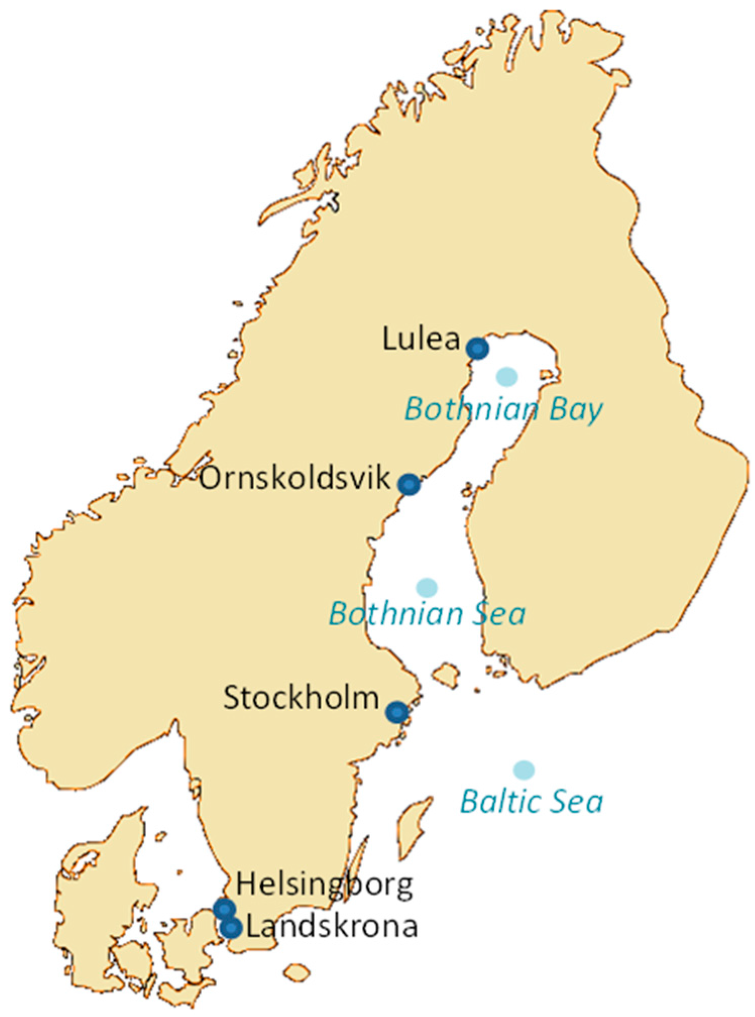
Figure 1.
Map over Sweden and different parts of the Baltic Sea. Key locations of IB Oden’s cruises and measurements are marked.
Figure 1.
Map over Sweden and different parts of the Baltic Sea. Key locations of IB Oden’s cruises and measurements are marked.

Figure 2.
Plot showing the measured gaseous elemental mercury (GEM) concentrations during the transit north from Helsingborg to Lulea.
Figure 2.
Plot showing the measured gaseous elemental mercury (GEM) concentrations during the transit north from Helsingborg to Lulea.

Figure 3.
Time series plot over GEM concentrations for IB Oden’s transit north from Helsingborg to Lulea.
Figure 3.
Time series plot over GEM concentrations for IB Oden’s transit north from Helsingborg to Lulea.

Figure 4.
Back trajectory for lower level found on 2 December. The measured GEM level was 1.213 ng/m3 at a vertical level of 20 m.
Figure 4.
Back trajectory for lower level found on 2 December. The measured GEM level was 1.213 ng/m3 at a vertical level of 20 m.

Figure 5.
Back trajectory for elevated level found on 5 December. Measured GEM level was 1.437 ng/m3 at a vertical level of 20 m.
Figure 5.
Back trajectory for elevated level found on 5 December. Measured GEM level was 1.437 ng/m3 at a vertical level of 20 m.
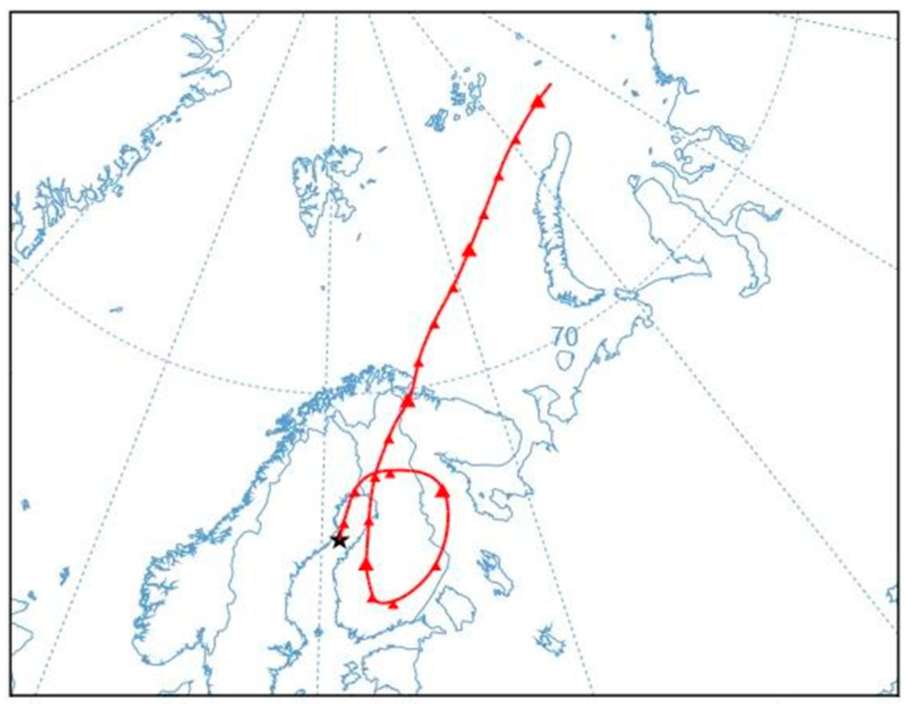
Figure 6.
Plot showing the measured concentrations of GEM during the first part of the icebreaking season, BB1, between 13 and 22 March.
Figure 6.
Plot showing the measured concentrations of GEM during the first part of the icebreaking season, BB1, between 13 and 22 March.

Figure 7.
Plot showing the measured concentrations of GEM during the second part of the icebreaking season, BB2, between 23 March and 5 April.
Figure 7.
Plot showing the measured concentrations of GEM during the second part of the icebreaking season, BB2, between 23 March and 5 April.
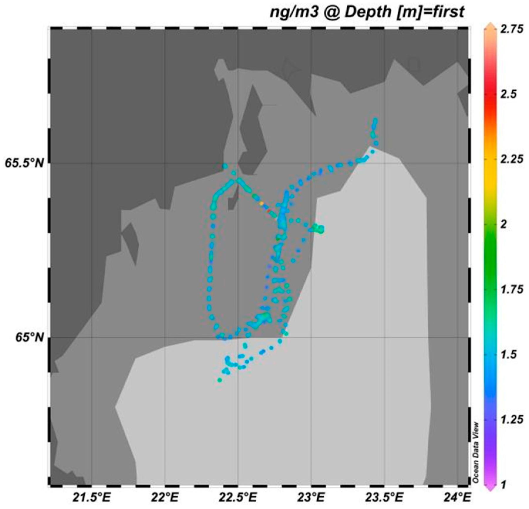
Figure 8.
Time series plot over GEM concentrations for BB1.
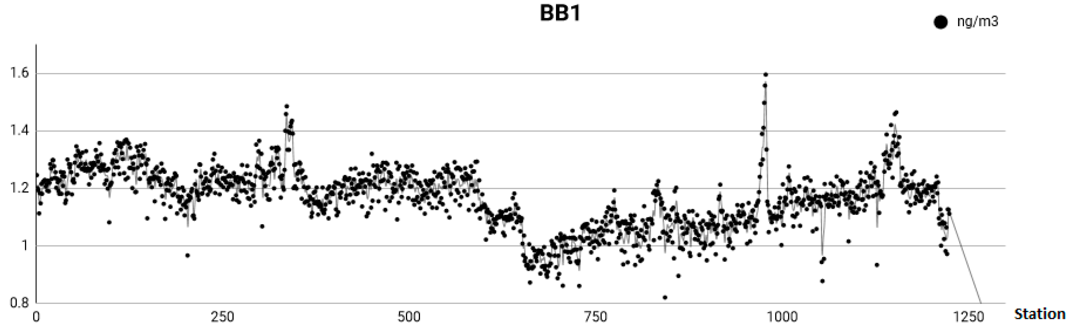
Figure 9.
Time series plot over GEM concentrations for BB2.
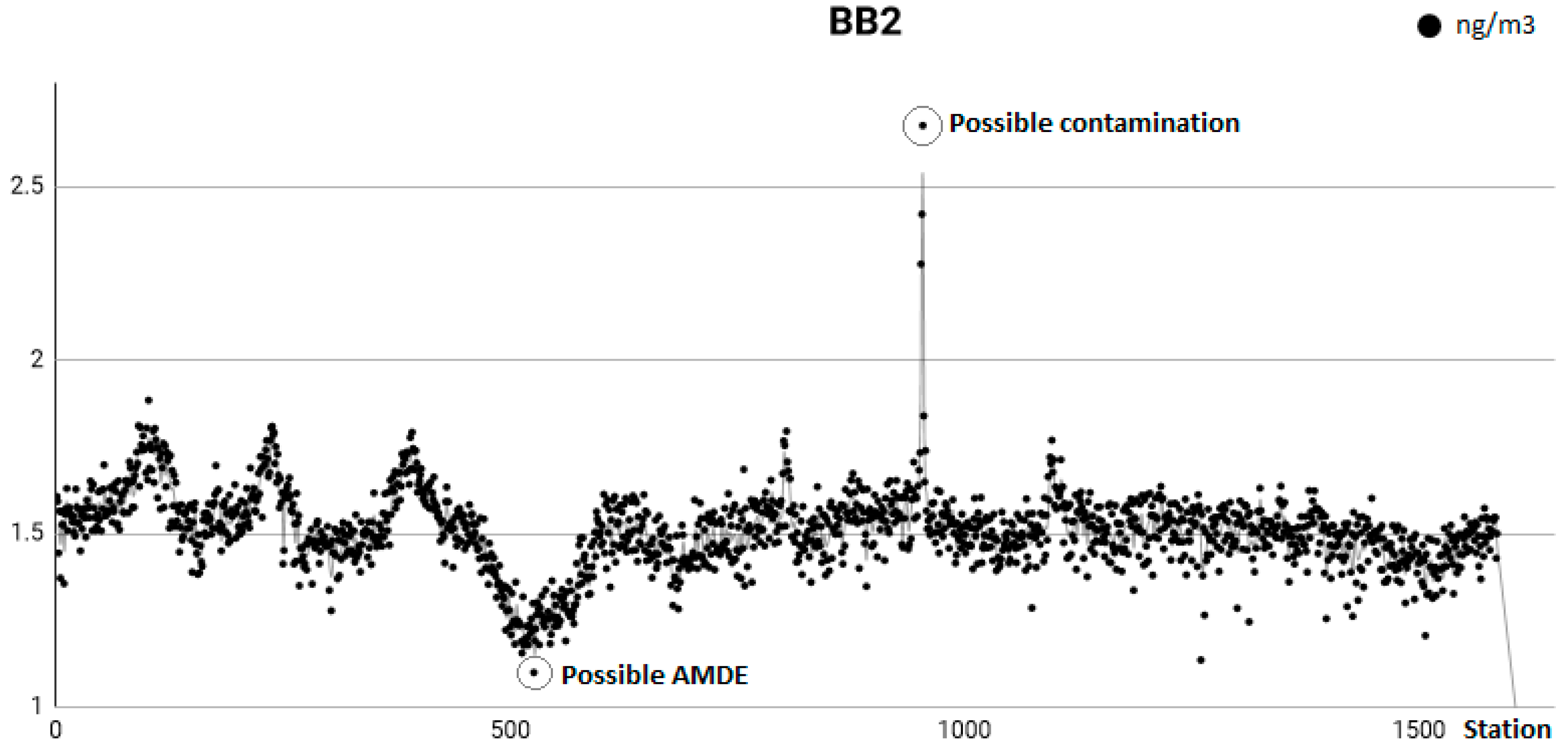
Figure 10.
Time series plot over GEM concentrations for BB3.
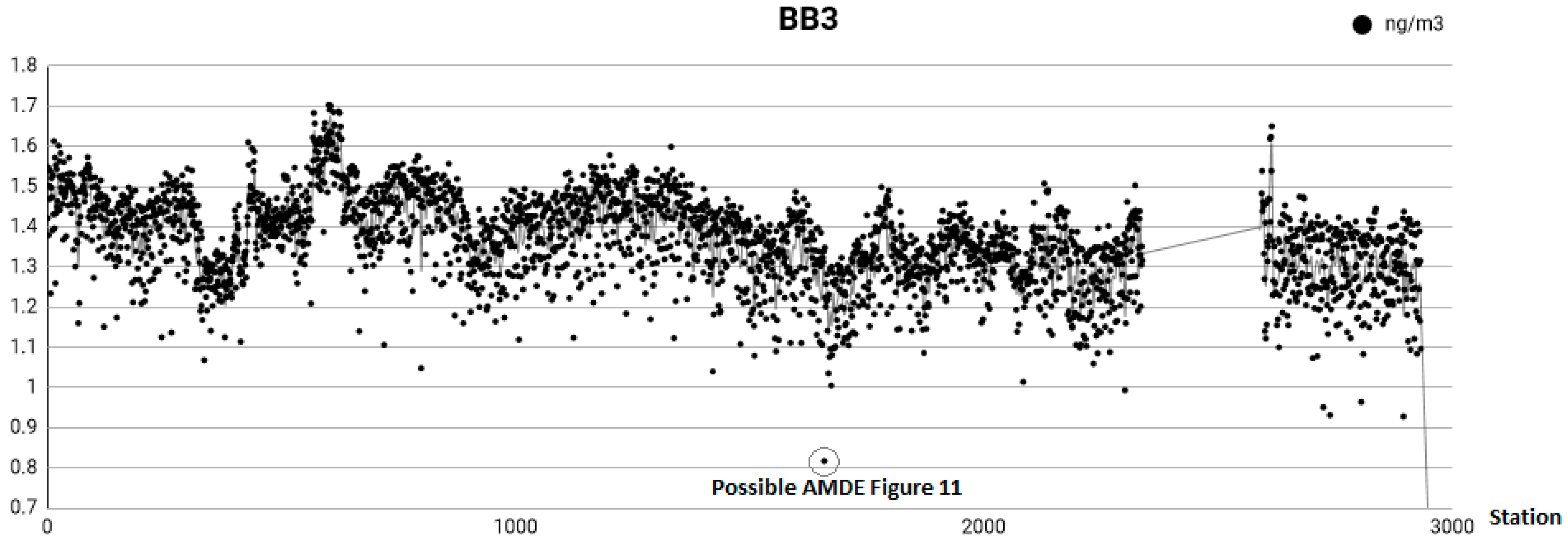
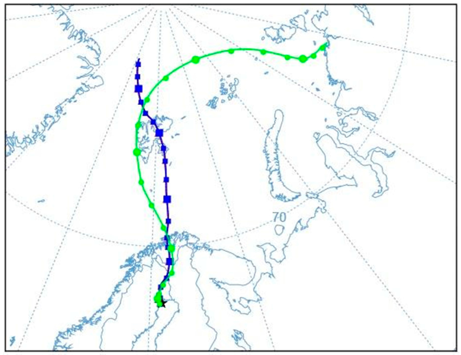
Figure 11.
Back trajectory for a possible atmospheric mercury depletion event (made) found on 18 April; the measured GEM level was 0.817 ng/m3. Blue line represents vertical level 20 m, green represents 100 m.
Figure 11.
Back trajectory for a possible atmospheric mercury depletion event (made) found on 18 April; the measured GEM level was 0.817 ng/m3. Blue line represents vertical level 20 m, green represents 100 m.

Figure 12.
Plot showing the measured concentrations of GEM during the transit south from Lulea to Landskrona.
Figure 12.
Plot showing the measured concentrations of GEM during the transit south from Lulea to Landskrona.
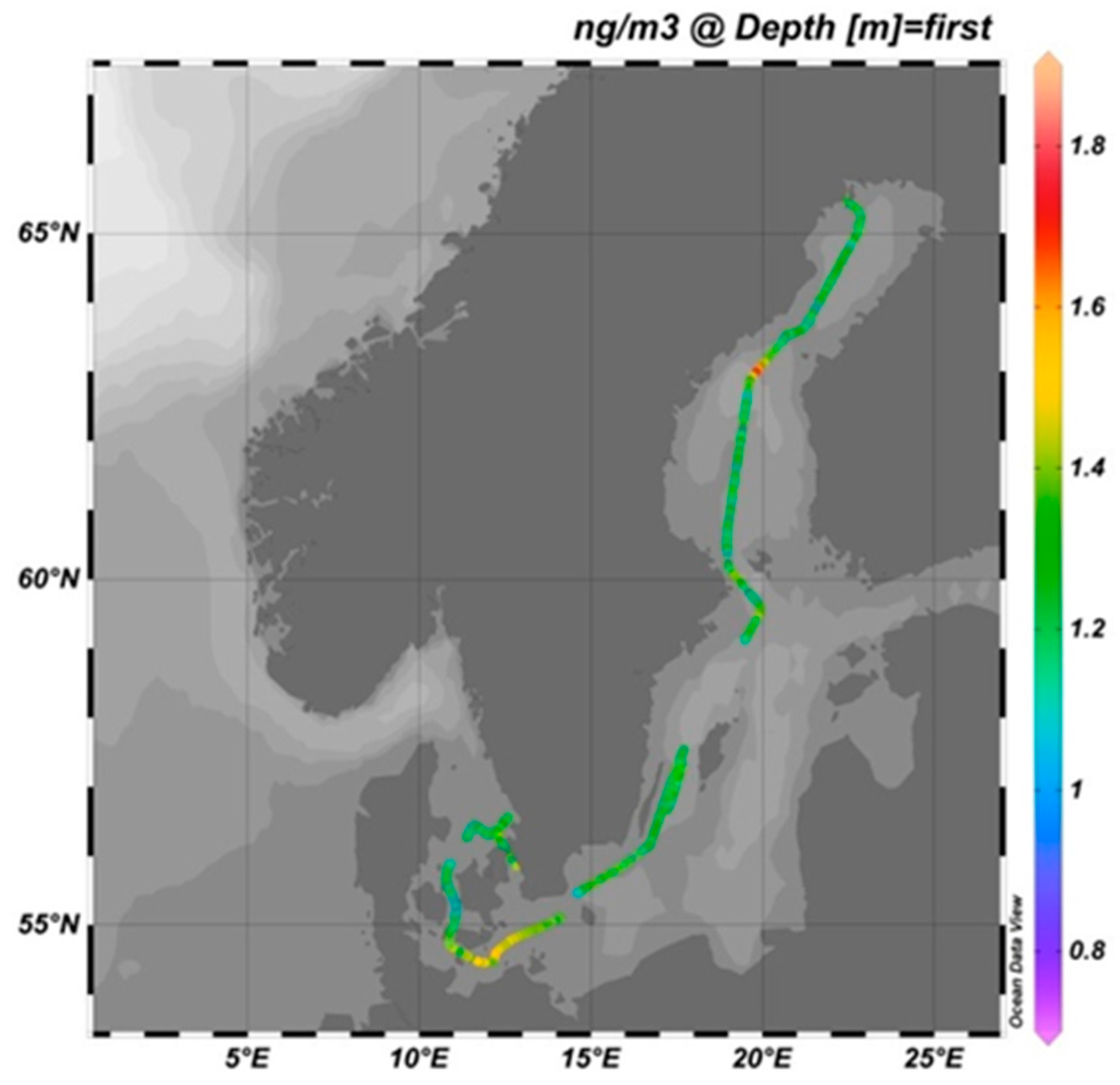
Figure 13.
Time series plot over GEM concentrations for IB Oden’s transit south from Lulea to Karlskrona.
Figure 13.
Time series plot over GEM concentrations for IB Oden’s transit south from Lulea to Karlskrona.

Figure 14.
Back trajectory for elevated level found on the 2 May. The measured GEM level was 1.558 ng/m3. Blue line represents vertical level 20 m, green represents 100 m.
Figure 14.
Back trajectory for elevated level found on the 2 May. The measured GEM level was 1.558 ng/m3. Blue line represents vertical level 20 m, green represents 100 m.

Figure 15.
Plot showing the north cruise with the same GEM concentration range as for Figure 16.
Figure 15.
Plot showing the north cruise with the same GEM concentration range as for Figure 16.

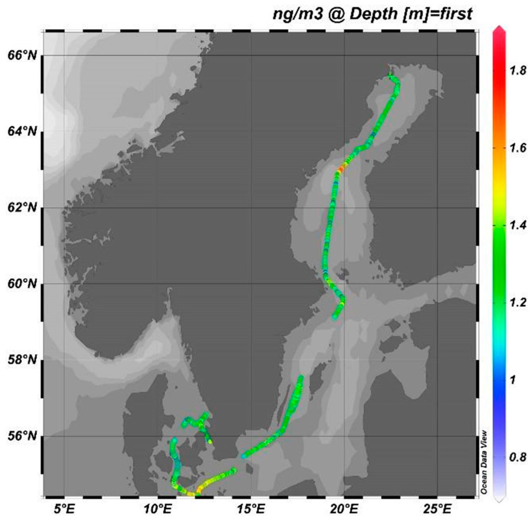
Figure 16.
Plot showing the south cruise with the same GEM concentration range as for Figure 15.
Figure 16.
Plot showing the south cruise with the same GEM concentration range as for Figure 15.

Table 1.
Results from the measurements performed in the Baltic Sea. Average values and standard deviations are presented.
Table 1.
Results from the measurements performed in the Baltic Sea. Average values and standard deviations are presented.
| Site | Season | GEM (ng/m3) | Range (Low-High, ng/m3) |
|---|---|---|---|
| Cruise North | Winter (2–6 December) | 1.36 ± 0.054 | 1.161–1.508 |
| Bothnian Bay (1) | Spring (13–22 March) | 1.16 ± 0.11 | 0.821–1.595 |
| Bothnian Bay (2) | Spring (23 March–5 April) | 1.51 ± 0.12 | 1.100–2.675 |
| Bothnian Bay (3) | Spring (6–27 April) | 1.36 ± 0.11 | 0.817–1.703 |
| Cruise South | Spring (28 April–5 May) | 1.29 ± 0.14 | 0.797–1.839 |
| All cruises | December 2016–May 2017 | 1.36 ± 0.16 | 0.817–2.675 |
Table 2.
Total gaseous mercury (TGM) levels from other studies where TGM was measured, in the northern hemisphere and around the world.
Table 2.
Total gaseous mercury (TGM) levels from other studies where TGM was measured, in the northern hemisphere and around the world.
| Location | Time Period | TGM (ng/m3) | Reference |
|---|---|---|---|
| Baltic Sea | Summer 1997 | 1.70 ± 0.20 | Wängberg et al. [19] |
| Baltic Sea | Winter 1998 | 1.38 ± 0.13 | Wängberg et al. [19] |
| Råö, Sweden | 2012–2015 | 1.42 ± 0.20 | Wängberg et al. [40] |
| Ny-Ålesund, Norway | 2015 | 1.49 ± 0.21 | Angot et al. [15] |
| Arctic | 2011–2014 | 1.46 ± 0.33 | Angot et al. [15] |
| Harwell, England | 2013 | 1.45 ± 0.24 | Kentisbeer et al. [41] |
| South China | May 2008–May 2009 | 2.80 ± 1.51 | Fu et al. [9] |
| Pallas, Finland | 1996–1997 | 1.26 | Berg et al. [42] |
| Ny-Ålesund, Norway | 1996–1997 | 1.43 | Berg et al. [42] |
| Hoburg, Sweden | 1979–1980 | 3.91 ± 1.15 | Brosset C. [23] |
| Mace Head, Ireland | Summer 1995–2001 | 1.6 | Ebinghaus et al. [21] |
| Mace Head, Ireland | Winter 1995–2001 | 1.9 | Ebinghaus et al. [21] |
© 2018 by the authors. Licensee MDPI, Basel, Switzerland. This article is an open access article distributed under the terms and conditions of the Creative Commons Attribution (CC BY) license (http://creativecommons.org/licenses/by/4.0/).
Share and Cite
MDPI and ACS Style
Hoglind, H.; Eriksson, S.; Gardfeldt, K. Ship-Based Measurements of Atmospheric Mercury Concentrations over the Baltic Sea. Atmosphere 2018, 9, 56. https://doi.org/10.3390/atmos9020056
AMA Style
Hoglind H, Eriksson S, Gardfeldt K. Ship-Based Measurements of Atmospheric Mercury Concentrations over the Baltic Sea. Atmosphere. 2018; 9(2):56. https://doi.org/10.3390/atmos9020056
Chicago/Turabian StyleHoglind, Hanna, Sofia Eriksson, and Katarina Gardfeldt. 2018. "Ship-Based Measurements of Atmospheric Mercury Concentrations over the Baltic Sea" Atmosphere 9, no. 2: 56. https://doi.org/10.3390/atmos9020056
Note that from the first issue of 2016, this journal uses article numbers instead of page numbers. See further details here.