Article

Model Performance Differences in Sulfate Aerosol in Winter over Japan Based on Regional Chemical Transport Models of CMAQ and CAMx

1
Central Research Institute of Electric Power Industry, Abiko, Chiba 270-1194, Japan
2
Department of Marine, Earth, and Atmospheric Sciences, North Carolina State University, Raleigh, NC 27607, USA
3
Graduate School of Maritime Sciences, Kobe University, Kobe, Hyogo 658-0022, Japan
4
National Institute for Environmental Studies, Tsukuba, Ibaraki 305-8506, Japan
5
Nagoya City Institute for Environmental Sciences, Toyota, Minami-Ku, Nagoya, Aichi 457-0841, Japan
6
Tokyo Metropolitan Research Institute for Environmental Protection, Koto-Ku, Tokyo 136-0075, Japan
*
Author to whom correspondence should be addressed.
Atmosphere 2018, 9(12), 488; https://doi.org/10.3390/atmos9120488
Submission received: 1 November 2018 / Revised: 30 November 2018 / Accepted: 7 December 2018 / Published: 10 December 2018
(This article belongs to the Section Aerosols)

Abstract

:
Sulfate aerosol (SO42−) is a major component of particulate matter in Japan. The Japanese model intercomparison study, J-STREAM, found that although SO42− is well captured by models, it is underestimated during winter. In the first phase of J-STREAM, we refined the Fe- and Mn-catalyzed oxidation and partly improved the underestimation. The winter haze in December 2016 was a target period in the second phase. The results from the Community Multiscale Air Quality (CMAQ) and Comprehensive Air quality Model with eXtentions (CAMx) regional chemical transport models were compared with observations from the network over Japan and intensive observations at Nagoya and Tokyo. Statistical analysis showed both models satisfied the suggested model performance criteria. CMAQ sensitivity simulations explained the improvements in model performance. CMAQ modeled lower SO42− concentrations than CAMx, despite increased aqueous oxidation via the metal catalysis pathway and NO2 reaction in CMAQ. Deposition explained this difference. A scatter plot demonstrated that the lower SO42− concentration in CMAQ than in CAMx arose from the lower SO2 concentration and higher SO42− wet deposition in CMAQ. The dry deposition velocity caused the difference in SO2 concentration. These results suggest the importance of deposition in improving our understanding of ambient concentration behavior.

1. Introduction

Three-dimensional air quality modeling is an important approach to improving our understanding of air pollutant behavior. Although modeling systems can represent emission, transport, chemical reactions, and deposition processes, there are uncertainties in these processes. Model intercomparison studies are valuable for understanding these uncertainties and can improve modeling performance. Based on the results and experience of Japanese projects, a model intercomparison project called Japan’s Study for Reference Air Quality Modeling (J-STREAM) was started [1], which has provided insights for improving modeling [2,3]. J-STREAM aims to establish reference air quality modeling for source apportionment and to formulate a strategy for mitigating air pollutants, including particulate matter with diameters of less than 2.5 μm (PM2.5) and photochemical ozone (O3), in Japan. The first phase focuses on understanding the ranges and limitations of PM2.5 and O3 concentrations simulated by participants using common input datasets. The first phase of J-STREAM was conducted on two specific weeks in each season from January 2013 to March 2014 to correspond with the government monitoring of PM2.5 [1]. We found that sulfate aerosol (SO42−), which is a major component of PM2.5 in Japan, is well captured by the models, but it is underestimated during winter. In the first phase of J-STREAM, we refined SO42− production via aqueous-phase reactions of O2 via Fe and Mn catalysis, and partly improved this underestimation [3]. We also demonstrated the importance of information about trace metals over Asia. Because more case studies of the model performance for PM2.5 and O3 are necessary, a second-phase model intercomparison analyzed the winter haze episode on 13–25 December 2016. Here, we present the model intercomparison based on the state-of-the-art regional models, Community Multiscale Air Quality (CMAQ) and Comprehensive Air quality Model with eXtensions (CAMx). This paper is organized as follows. The model setups of CMAQ and CAMx are presented in Section 2. The model simulation results are compared with the observations in Section 3, and we explain the differences between the models focusing on deposition. Finally, the conclusions from this study and future perspectives are discussed in Section 4.

2. Modeling Design

In the second phase of J-STREAM, the winter haze episode from 13 to 25 December 2016 was focused on. In the model simulation, a seven-day spin-up time from 6 December was used, and the domain and the common input dataset of meteorology and emissions were the same as for the first phase of J-STREAM [1]. The vegetation database for Japan was introduced, and this revision helped to improve the meteorological fields and the emissions of biogenic volatile organic compounds [2]. For the emissions inventory, compositions of metal elements in PM2.5 were considered over Asia based on composition reports [4] because our findings in the first phase suggested that trace metals over Asia should be included [3]. CMAQ version 5.0.2 [5] model simulations were performed in this study. The gas and aerosol chemistry was handled by SAPRC07 and AERO6, respectively [3]. CMAQ version 5.0.2 treats one gas-phase chemical reaction and five aqueous-phase chemical reactions involved in SO42− production [6]. A total of five aqueous-phase chemical pathways for SO2 oxidation in clouds, involving hydrogen peroxide, O3, oxygen (O2) via Fe and Mn catalysis, methyl hydrogen peroxide, and peroxyacetic acid, were included. The original configuration (base-case) of CMAQ was simulated first. In our previous study [3], we refined the aqueous-phase oxidation pathway of O2 via Fe and Mn catalysis by increasing Fe and Mn solubilities, and considering pH dependency in the reaction constants. The details of these modifications are described in our previous study, and this refinement partly improved the model performance; however, SO42− is still underestimated in winter [3]. We performed this sensitivity simulation next (sensitivity simulation A). In addition, as we mentioned in previous future perspectives [3], the aqueous-phase reaction pathway via NO2 was incorporated into CMAQ considering the neutralized or acidic features of aerosols in Asia [7,8]. The rate constant expression of the aqueous-phase NO2 oxidation pathway is introduced as
d [ S ( IV ) ] / dt   =   k   [ NO 2 ( aq ) ] [ S ( IV ) ] ,
where k has been measured as from (0.14–2.00) × 106 M−1 s−1 between pH 5.0 and 5.8 [9] to (1.24–1.67) × 107 M−1 s−1 between pH 5.3 and 8.7 [10]. We used the latter value range, which was a considerable maximum increase via the NO2 oxidation pathway. For this rate constant, the dependency on pH is considered as
k   =   1.24   ×   10 7   M 1   s 1   ( pH   <   5.3 ) ,   k   =   1.67   ×   10 7   M 1   s 1   ( pH   >   8.7 ) ,
where for the range pH 5.3–8.7, the rate constant was linearly interpolated. A simulation including this additional aqueous-phase NO2 oxidation pathway was performed (sensitivity simulation B). A summary of the CMAQ sensitivity simulations is listed in Table 1.
Due to the uncertainties in the model, a comprehensive comparison with other models is important. In this study, a simulation by CAMx version 6.4 [11] was also performed. The meteorological fields were prepared from the unified input dataset for the J-STREAM project, and to be consistent with the CMAQ modeling system, the ACM2 method for diagnosing the vertical diffusivities was selected in the interpreprocessor for meteorology in CAMx. The gas chemistry was based on the SAPRC07, and the aerosol chemistry was based on the CF scheme, which divides the size distribution into two static coarse- and fine-mode aerosols. The emission input data was also consistent with the CMAQ modeling system, except for the consideration of trace metals, because the version of CAMx used in this study does not explicitly treat trace metals. Instead, the ratios to total particulate matter of 3.355% for Fe and 0.115% for Mn were used to calculate the Fe- and Mn-catalyzed oxidation process in the CAMx modeling system. The one gas-phase chemical reaction and five aqueous-phase reactions were identical to those in CMAQ. For Fe- and Mn-catalyzed oxidation, CAMx used the same pH dependency expression as in sensitivity simulation A in CMAQ [3]. The difference in the SO42− production process between sensitivity simulations A by CMAQ and CAMx was the concentration of trace metals needed for Fe- and Mn-catalyzed oxidation and the calculation of pH status. CMAQ sensitivity simulation B was expected to produce a higher SO42− concentration than CAMx due to the additional NO2 aqueous oxidation pathway. Note that the windblown dust simulation was not performed in CMAQ or CAMx in this study.

3. Results and Discussion

3.1. Model Performance during Winter Haze

The spatial distribution of SO42− concentration over domain 1 of J-STREAM with 45 km horizontal grid resolution during the winter haze period from the base-case CMAQ simulation and the changes in sensitivity simulations A and B are shown in Figure 1. The high concentration over the Asian continent that stretched into the downwind region of Japan was related to the transboundary SO42− in Japan, as we have previously discussed [12,13,14,15,16]. Generally, the SO42− concentrations over the whole of East Asia were increased in sensitivity simulations A and B. Higher increases of over 5% compared with the base-case simulation were found above the south part of the mainland of China, from northeast China to northern Japan, and from central China (e.g., Yangtze River Delta region) to the East China Sea. These increases were larger in sensitivity simulation B than in A due to the increased oxidation pathway via NO2.
To evaluate these increased concentrations, the observation data from Shenyang in northeast China (monitoring station at 123.412° E, 41.731° N; gray star in Figure 1) were used [17]. In this study [17], the PM composition was investigated during several haze events, and 17 December 2016, 00:00 to 21 December 2016, 14:00 was classified as a haze event. This event corresponded to the period that we focus on in the present work. The results are shown in Figure 2 and the observed mean SO42− concentration during the haze event at Shenyang was 37.9 μg/m3.
From the CMAQ model results, the mean concentration for the base-case simulation was 28.50 μg/m3, and this was increased to 32.13 μg/m3 in sensitivity simulation A, and to 33.13 μg/m3 in sensitivity simulation B (Figure 1). Other statistical metrics (maximum, upper and lower quartiles, and median) also showed the increase compared with the base-case simulation; however, the minimum value was similar. This implied that the background SO42− concentration was not related to the chemical production, and was related to the boundary condition. The mean value from CAMx was 35.81 μg/m3, which was larger than that from CMAQ. Similar model reproducibility between CMAQ and CAMx has also been reported over the United States in a model intercomparison study [18,19]. Even in CMAQ sensitivity simulation B, in which the SO42− production process was increased further, CAMx simulated a higher concentration. In the aqueous-phase Fe- and Mn-catalyzed oxidation reaction in the SO42− oxidation pathway, the Fe and Mn concentrations were different in CMAQ and CAMx in sensitivity simulation A. Over domain 1, the surface mean concentrations in CMAQ and CAMx were 61.79 and 60.47 ng/m3 for Fe, and 1.62 and 2.06 ng/m3 for Mn, respectively. The concentrations and spatial distributions of Fe and Mn were similar in the two models. Therefore, the higher oxidation in CAMx via Fe- and Mn-catalyzed oxidation did not explain the higher concentration calculated by CAMx. The variation range of CAMx was larger than that of CMAQ. CAMx had a larger maximum and upper quartile and a smaller median and lower quartile than CMAQ.
The nested domains in J-STREAM covering Japan were compared further. Domain 2 of J-STREAM covers the whole of Japan with 15 km horizontal grid resolution. Although the analyzed period does not correspond to the 2 weeks of intensive observation recommended by the Ministry of the Environment, Japan, the network observations from the Acid Deposition Monitoring Network in East Asia (EANET) are available for the target period in December 2016. In EANET, the atmospheric concentrations of aerosols are measured by the four-stage filter pack method. The SO42− aerosol measured on the Teflon filter in the first stage is determined by ion chromatography. The sampling period of this filter pack method was 1 to 2 weeks [20]. To exclude the effect of sea salt, Na+ was used as a sea-salt tracer and non-sea-salt SO42− (referred to as SO42− hereafter for simplicity) was calculated. In December 2016, most EANET sites in Japan conducted their observations from 12 to 26 December 2016. The corresponding times at each observation site were analyzed in the model results. There were nine available sites, of which seven sites were remote sites according to the EANET classification, and the Ijira site was rural and the Tokyo site was urban.
The spatial distribution of the results from the four models showed a high concentration over the Asian continent, and the concentrations over Japan were in the range 0.5–3.0 μg/m3 (Figure 3 (top)). The increase in the SO42− concentration in CMAQ above the Sea of Japan was around 3.0 μg/m3 in the base-case CMAQ simulation, 3.5–4.0 μg/m3 in CMAQ sensitivity simulation A, and 4.0–4.5 μg/m3 in CMAQ sensitivity simulation B, which stretched into northern Japan. The comparison of the EANET observations and results from the four models are shown as bar graphs (Figure 3 (bottom)). Generally, the models captured the observed high and low concentrations. Model overestimations were found at Happo and Ogasawara. Happo is a mountainous site with clean air, and the models had difficulty in capturing the low SO42−concentrations. Ogasawara is located in the northwest Pacific, and the models overestimated the concentration due to the overestimation of the stretched high-concentration plume from the Asian continent, as found in the spatial distribution. In contrast, large model underestimations were found at Sadoseki, Tappi, and Rishiri in northern Japan. Considering the modeled spatial distribution, the high concentration from the Asian continent should prevail over northern Japan to explain this underestimation; CAMx performed well, especially at Tappi, based on the spatial distribution.
For the comparison with EANET observation sites, the model reproducibility was judged by statistical analysis based on the correlation coefficient (R) with the significance level determined by Students’ t-test, mean fractional bias (MFB), and mean fractional error (MFE). The statistical analysis results are listed in Table 2. The correlations of the model results with the observations were 0.51–0.59 for CMAQ and 0.70 for CAMx. The CMAQ base-case simulation and sensitivity simulation A were not statistically significant, but CMAQ sensitivity simulation B and CAMx showed statistical significances of p < 0.1 and p < 0.05, respectively. The model performance goals were proposed as MFB ≤ ±30% with MFE ≤ +50% for the best model performance, and model performance criteria were proposed as MFB ≤ ±60% with MFE ≤ +75% for the acceptable model performance [21]. The CMAQ base-case simulation meets the model performance criteria, and the other three models meet the model performance goals. The improvements in CMAQ model performance from the base-case simulation to sensitivity simulations A and B were confirmed statistically. Based on the MFB, CAMx simulated higher SO42− concentrations compared with the CMAQ models, as found at the Shenyang site in China (Figure 2).
The comparison of the finest nested domain in J-STREAM was investigated further. Domains 3 and 4 of J-STREAM cover the Kansai (including Osaka and Nagoya) and Kanto (including Tokyo) regions, respectively, with a 5 km horizontal grid resolution. At the Nagoya City Institute for Environmental Sciences (located at 136.92° E, 35.10° N; hereafter called the Nagoya site) and the Tokyo Metropolitan Research Institute for Environmental Protection (located at 139.82° E, 35.67° N; hereafter called the Tokyo site), daily PM2.5 samples are collected from 10:00 local time to 10:00 the next day. In addition, an aerosol chemical speciation analyzer (ACSA) automated monitoring system at Mukoujima (located at 139.81° E, 35.71° N) conducts hourly SO42− measurements. This automated monitoring system has been compared with a model in our previous study [22]. The results of CMAQ sensitivity simulation B and CAMx and their comparison with the observation data from Nagoya and Tokyo are shown in Figure 4. Comparing the same spatial distribution as in domain 2 in Figure 3 showed that CAMx generally gave a higher concentration than CMAQ over the whole of domains 3 and 4. Based on the comparison of the temporal variation of daily mean SO42− concentration at Nagoya, the observations showed the highest concentration on 18 December 2016, whereas all the models showed the highest concentrations on 21 December 2016. In the second phase of J-STREAM, participants could also use their own meteorological input dataset instead of the unified input; however, other meteorological fields did not explain this discrepancy between the observed and modeled peaks at Nagoya [23]. To explain the discrepancy in the high-concentration episode, further investigation is required in future studies. The comparison of the simulated and observed concentrations at Tokyo showed that all four models almost exactly captured the timing and concentrations of the peaks on 18 and 21 December 2016.
The model performances at these three sites in the finest modeling domains were also judged by statistical analysis based on R, MFB, and MFE. The results of statistical analysis including the base-case simulation and CMAQ sensitivity simulation A are listed in Table 3. At Nagoya, R was around 0.6 and with a statistical significance of p < 0.05, and all models met the model performance goal based on MFB and MFB. At Tokyo, the time series comparison suggested that R was greater than 0.9, and all models met the model performance goal. At Mukoujima, compared with the hourly dataset, the CMAQ models met the model performance goal, and the CAMx model met the model performance criteria because the concentrations were higher than those of CMAQ. The CMAQ models gave lower concentrations than the CAMx model. At the urban sites in Japan, the increased concentrations in the CMAQ sensitivity simulations were 0.02–0.06 μg/m3; lower than the increased concentrations at the EANET observation sites. If there are local oxidations via an enhanced production process, the concentration should be increased at these urban sites. The results suggested that factors in the CMAQ sensitivity simulation may be more important for capturing the transboundary transport than local production in Japan. This may be because the concentrations of Fe, Mn, and NO2 in Japan are much lower than those over Asia.

3.2. Differences between CMAQ and CAMx

Based on the CMAQ base-case and sensitivity simulations and their comparison with observation data from EANET, Nagoya, and Tokyo, we found that the sensitivity simulation including the enhancement of the Fe- and Mn-catalyzed oxidation pathway and aqueous-phase NO2 oxidation improved the CMAQ model performance. Comparing CMAQ and CAMx showed that CMAQ tended to simulate lower concentrations over most of Japan. The differences in concentration between CMAQ sensitivity simulation B and CAMx are highlighted by the substituted (CMAQ−CAMx) spatial distribution shown in Figure 5. In this section, we investigate these differences further. Because the emission and meteorology input data for these CMAQ and CAMx simulations are unified for the model intercomparison, the differences may be explained by the models themselves. We focus on deposition processes for SO42− and also SO2, a precursor of SO42−.

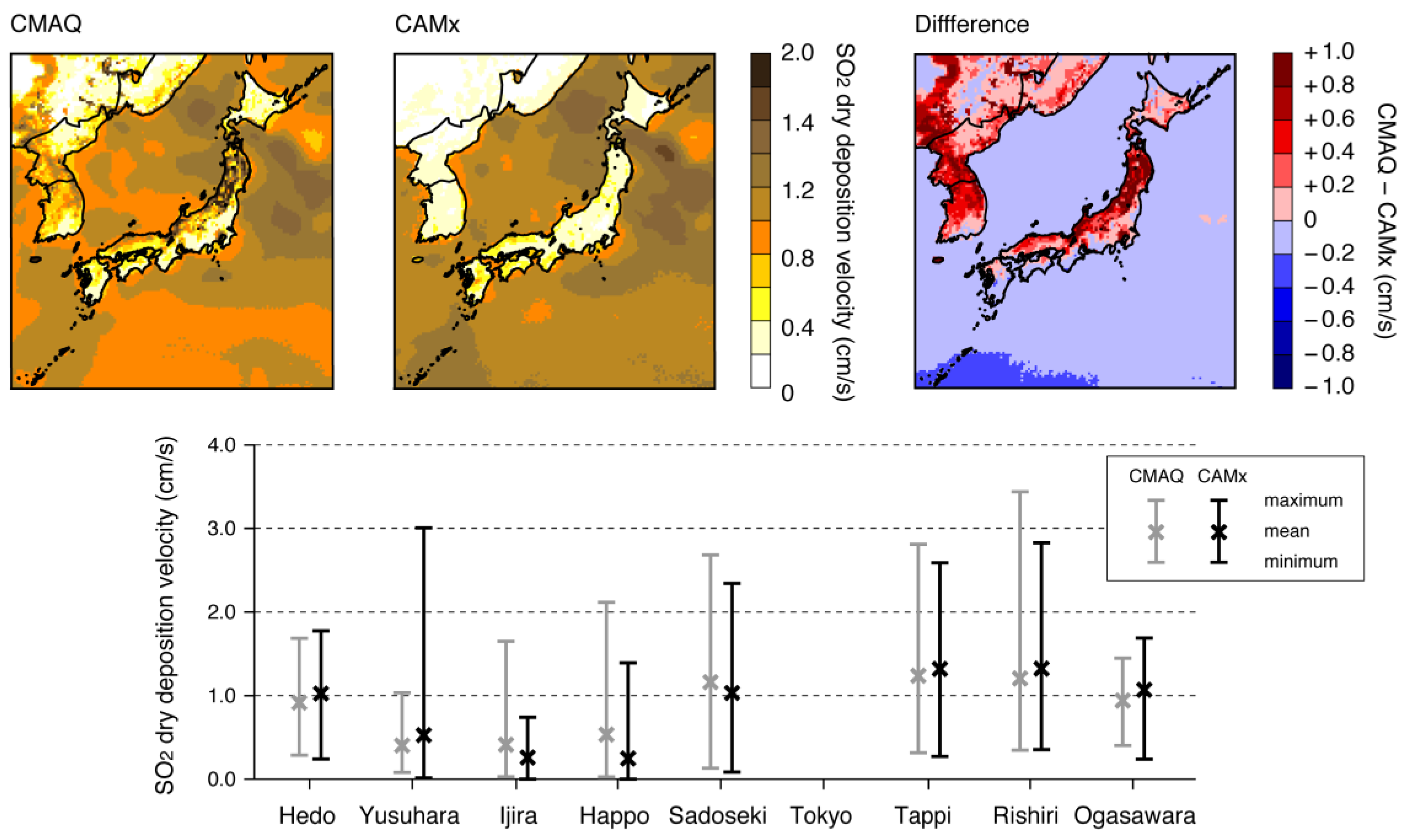
3.2.1. Dry Deposition of SO2

First, we focus on SO2, a precursor of SO42−. Figure 6 shows the modeled SO2 concentrations over domain 2 and the differences between CMAQ sensitivity simulation B and CAMx. CMAQ gave lower SO2 concentrations over land and CAMx gave slightly higher SO2 concentrations over ocean. The differences in SO2 concentration were within 1 ppbv over Japan. For the EANET observations, the ambient SO2 concentrations are measured with automatic instruments based on the ultraviolet fluorescent method [20]. The data are provided as hourly data with the first decimal place on the unit of ppbv; hence, the SO2 concentrations simulated by CMAQ and CAMx were also compared after rounding. The results are also shown in Figure 6. Compared with the mean observation value, all models overestimated the values and were within or comparable to the observed maximum. Generally, in the spatial distribution, CMAQ also modeled lower concentrations than CAMx at EANET observation sites. In the CMAQ models, SO2 concentrations decreased from the base-case to sensitivity simulations A and B because the aqueous-phase oxidation pathways from SO2 to SO42− were increased in the CMAQ simulations.
Modeled dry deposition velocity was investigated to examine the factors that produced these model behaviors in CMAQ and CAMx for SO2. The dry deposition schemes used in CMAQ and CAMx were M3DRY [24] and the scheme reported by Zhang et al. [25], respectively. Both schemes invoke the three resistances model of the aerodynamic, boundary, and surface resistances. CMAQ used 24 land-use categories as defined by the United States Geological Survey, whereas CAMx internally mapped in 26 land-use categories, and these led to the surface resistance. The spatial distribution and the model comparison at EANET observation sites are shown in Figure 7. For the dry deposition velocity, the CMAQ estimation was higher than that of CAMx over land, whereas the CMAQ estimation was lower compared with CAMx over the ocean. This was the opposite trend to that for the SO2 concentration. The average SO2 dry deposition velocities at EANET sites were around 1 cm/s, ranging from near 0 to around 3 cm/s. From the estimation based on the inferential method at EANET sites over Japan during 2003–2008, SO2 dry deposition velocities were reported as 0.6–2.8 cm/s over forest and 0.2–1.2 cm/s over grass [26]. Although the modeled values corresponded well to these observation-based values, the model overestimated the observed mean value of EANET. This result suggests that the oxidation process should be increased further.
The spatial correlation between the differences in SO2 concentration are shown in Figure 6 and the differences in SO2 dry deposition velocity shown in Figure 7 were −0.46 over domain 2. We concluded that the lower SO2 concentration modeled by CMAQ compared with CAMx was attributed to the higher SO2 dry deposition velocity modeled by CMAQ compared with CAMx. The differences in modeled SO2 concentration were within 1 ppbv over Japan; however, this could explain the modeled differences in SO42− concentration. Detailed analyses were conducted over domains 3 and 4. The comparison of SO2 concentration over domains 3 and 4 modeled by CMAQ sensitivity simulation B and CAMx and the difference are shown in Figure 8. The spatial distribution patterns of SO2 concentration modeled by CMAQ and CAMx were similar; there were higher concentrations greater than 5 ppbv along the coastline over sources of SO2 emissions, such as power plants and industrial areas. The difference in spatial distribution indicated that CMAQ generally produced lower SO2 concentrations than CAMx, especially over land. The higher SO2 concentrations from CMAQ were found near power plants and industrial areas. Because these sources were characterized as having elevated emission heights, investigating the vertical distribution in models will be important to gain further insights, and well-coordinated measurements are required to achieve this. To explain the differences in model behavior of SO42− concentration, the differences in SO42− concentration and SO2 concentration between CMAQ sensitivity simulation B and CAMx were used to construct a scatter plot. The scatter plot showed that the negative difference in SO42− concentration (lower SO42− concentration in CMAQ compared with CAMx) was related to the negative difference in SO2 concentration (lower SO2 concentration in CMAQ compared with CAMx) to some extent. The difference in the SO2 precursor was an important factor in explaining the differences in modeled SO42− concentrations, and the difference in SO2 concentration was caused by differences in dry deposition velocity. The SO42− and SO2 concentrations were not clearly related, especially in the case of the difference in SO2 concentration close to zero; hence, we sought other explanations of the SO42− deposition process.

3.2.2. Wet Deposition of SO42−

The main deposition process that removes SO42− from the atmosphere to the surface is wet deposition, as has been suggested by observations [24] and our previous study [18]. The accumulated dry and wet depositions during the analyzed period were calculated, and the wet deposition as a fraction of the total deposition is shown in Figure 9. During the analyzed period in wintertime, both CMAQ and CAMx showed that the wet deposition process was dominant. Although some regions (e.g., the Asian continent and Pacific Ocean) showed comparable or dominant dry deposition, wet deposition was mainly identified as the dominant deposition process over Japan, with a fraction above 90%.
In EANET, wet deposition of aerosols is measured by automated wet-only samplers and the SO42− concentration in precipitation is determined by ion chromatography [27]. The sampling period for wet deposition is daily at EANET sites in Japan, except at Ijira, where it is fortnightly. The wet depositions of SO42− modeled by CMAQ and CAMx were compared with each other and with the EANET observations (Figure 10). The CMAQ and CAMx spatial distributions showed that simulated wet deposition was high over western Japan and eastern Japan over the Pacific regions, and these features were similar for CMAQ and CAMx. However, CMAQ showed higher wet deposition over Japan, except in northern Japan, and over the Asian continent, whereas CMAQ showed lower wet deposition over the East China Sea and Sea of Japan. Compared with the monitoring network over Japan, CMAQ models showed higher wet deposition and CAMx showed lower wet deposition. The CMAQ sensitivity simulations showed that enhanced aqueous-phase oxidation led to higher wet deposition. The statistical analyses with the observations are summarized in Table 4. Both models showed general correspondence with the observations, with R of around 0.7 and statistical significance of p < 0.05. The mean and MFB values confirmed that SO42− wet deposition was overestimated by the CMAQ models and underestimated by the CAMx model compared with the observations. The model performance for precipitation can be an important factor in the model performance for wet deposition. Taking into account this uncertainty, the adjusted approach, in which the precipitation amount is linearly scaled to match the observations, has been used in previous studies [16,28,29]. In this study, the modeled wet deposition accumulated over the analyzed period was adjusted based on
Adjusted   wet   deposition   =   p e r i o d ( w e t   d e p o s i t i o n ) × p e r i o d ( o b s e r v e d   p r e c i p i t a t i o n ) p e r i o d ( m o d e l e d   p r e c i p i t a t i o n )
Figure 10 also shows the modeled and observed precipitation during the analyzed period. The models underestimated the precipitation amount, except at the Sadoseki and Rishiri sites. Table 4 summarizes the statistical analysis based on the adjusted wet deposition. The mean wet deposition, and hence MFB, were increased in both CMAQ and CAMx. In addition, CMAQ overestimated SO42− wet deposition, whereas CAMx underestimated it over EANET sites, even accounting for the differences between the observed and modeled precipitation. Although the meteorological fields used in these model intercomparisons are unified and the SO42− oxidation pathway is identical, the calculation criteria for the aqueous-phase reactions and wet deposition are different in these models. The liquid water content used to identify the presence of cloud is defined as the sum of cloud water, rain, and graupel mixing ratio in CMAQ, whereas in CAMx, it is defined as the sum of cloud water and ice mixing ratio with the linear ramp function between the freezing points of 233 and 273 K. The threshold values for calculating the aqueous-phase reactions and wet depositions are 0.01 g/m3 in CMAQ and 0.05 g/m3 in CAMx. The effects of these fundamental differences between models should be investigated in future work. In summary, CMAQ generally showed lower SO42− concentrations than CAMx due to the higher SO42− wet deposition.
Differences in SO42− concentration were found at Nagoya and Tokyo compared with the high temporal resolution observations; therefore, the analysis for SO42− wet deposition was done over J-STREAM domains 3 and 4, and the results are shown in Figure 11. Comparing the differences between CMAQ and CAMx showed that CMAQ modeled higher SO42− wet deposition than CAMx over almost all of domains 3 and 4. The scatter plots of the differences in SO42− concentration and SO42− wet deposition over domains 3 and 4 both indicated that most of the grid data showed negative differences for SO42− concentration (lower concentration for CMAQ compared with CAMx) and positive difference for SO42− wet deposition (higher wet deposition for CMAQ compared with CAMx). The results showed that the other important factor that explained the differences in SO42− concentration between CMAQ and CAMx was SO42− wet deposition at EANET observation sites and over domains 3 and 4. A model intercomparison in Europe also concluded that the accurate estimate of deposition is key to an accurate simulation of ambient concentrations [30].

4. Conclusions and Future Perspectives

The Japanese model intercomparison study, J-STREAM, found that although SO42− is generally well captured by models, it is underestimated during winter. In our previous study in the first phase of J-STREAM, we improved the modeled SO42− concentration during winter in Japan by focusing on the Fe- and Mn-catalyzed oxidation pathway [3]. In the present study, we investigated the reason for the underestimation further via the model intercomparison of two state-of-the-art regional chemical transport models, CMAQ and CAMx. In CMAQ, in addition to the enhancement of the Fe- and Mn-catalyzed oxidation pathway, the aqueous-phase NO2 oxidation pathway was included. The CMAQ sensitivity simulations and the comparison with the observation data over Japan improved the performance of CMAQ. Despite the increased Fe- and Mn-catalyzed oxidation pathway and NO2 aqueous reaction, CMAQ tended to model lower SO42− concentrations over Japan than CAMx. Detailed comparisons showed that this difference between CMAQ and CAMx arose from the differences in SO2 concentration and SO42− wet deposition at EANET sites and over domains 3 (Kansai region) and 4 (Kanto region). Scatter plots were constructed to explain the differences, and the negative differences in SO42− concentration (lower concentration in CMAQ compared with CAMx) were related to the negative differences in SO2 concentration (lower concentration in CMAQ compared with CAMx) and positive differences in SO42− wet deposition (higher wet deposition in CMAQ compared with CAMx). We focused on the deposition because the model input datasets (e.g., emissions and meteorological field) are unified in the J-STREAM framework.
As we discussed in relation to the common model underestimation at Nagoya (Figure 4), further studies of the effects of meteorological parameters are needed, and this direction was also suggested by another model intercomparison study in Europe [31]. Another important factor is the vertical distribution of air pollutants simulated by the models. Differences in elevated emission sources between models were found (Figure 8). Thus, model evaluations of the vertical distribution are required; the intensive ozonesonde observations in J-STREAM could provide valuable data for this research. In addition, ongoing development of modeling updates [32,33] will be included in our future model intercomparison study. The recent dramatic decline in anthropogenic SO2 emission changes in China should be considered [34,35,36,37], because the Asian emission inventory has not been updated from 2010 in the second phase. The decline in SO2 emissions from China may also cause the underestimation of SO42− concentration. Therefore, an additional pathway of oxidation via heterogeneous chemistry is expected to be important [38,39,40]. Through this study, we proposed a way to improve the model performance during winter, although more case studies are needed to improve our knowledge of the behavior of SO42− in Japan based on both ambient concentrations and deposition processes.

Author Contributions

S.I. coded the additional aqueous-phase reactions in the CMAQ model, conducted the model simulations and comparison of the models with observations, and wrote this paper; K.Y. is the subleader of the model intercomparison, and prepared the meteorological inputs and initial and boundary conditions; H.H. is the subleader of the inorganic aerosol measurements and contributed to the submodel development, and conducted the ACSA observations at Mukoujima, Tokyo; K.H. and S.S. took the daily PM2.5 samples at Nagoya City Institute for Environmental Sciences and Tokyo Metropolitan Research Institute for Environmental Protection, respectively; S.C. is the leader of the J-STREAM project, and prepared the emission inputs and discussed the model intercomparison results.

Funding

This research was funded by the Environment Research and Technology Development Fund (5-1601) of the Environmental Restoration and Conservation Agency.

Acknowledgments

This research was supported by the Environment Research and Technology Development Fund (5-1601) of the Environmental Restoration and Conservation Agency. The daily SO42− data from Nagoya City Institute for Environmental Sciences and Tokyo Metropolitan Research Institute for Environmental Protection were obtained by collaboration with the research group under the Environment Research and Technology Development Fund (5-1604) of the Environmental Restoration and Conservation Agency, led by Prof. Kazuo Osada at Nagoya University. The authors appreciate the helpful comments on trace metals over Asia from Prof. Shuxiao Wang and Prof. Jia Xing at Tsinghua University, China, and Dr. Hu Xiao at the University of Hong Kong.

Conflicts of Interest

The authors declare no conflict of interest.

References

  1. Chatani, S.; Yamaji, K.; Sakurai, T.; Itahashi, S.; Shimadera, H.; Kitayama, K.; Hayami, H. Overview if model inter-comparison in Japan’s study for reference air quality modeling (J-STREAM). Atmosphere 2018, 9, 19. [Google Scholar] [CrossRef]
  2. Chatani, S.; Okumura, M.; Shimadera, H.; Yamaji, K.; Kitayama, K.; Matsunaga, S. Effects of a detailed vegetation database on simulated meteorological fields, biogenic VOC emissions, and ambient pollutant concentrations over Japan. Atmosphere 2018, 9, 179. [Google Scholar] [CrossRef]
  3. Itahashi, S.; Yamaji, K.; Chatani, S.; Hayami, H. Refinement of modeled aqueous-phase sulfate production via the Fe- and Mn-catalyzed oxidation pathway. Atmosphere 2018, 9, 132. [Google Scholar] [CrossRef]
  4. Fu, X.; Wang, S.; Zhao, B.; Xing, J.; Cheng, Z.; Liu, H.; Hao, J. Emission inventory of primary pollutants and chemical speciation in 2010 for the Yangtze River Delta region, China. Atmos. Environ. 2013, 70, 39–50. [Google Scholar] [CrossRef]
  5. US EPA Office of Research and Development. Community Multiscale Air Quality (CMAQ) Model Version 5.0.2; US EPA Office of Research and Development: Washington, DC, USA, 2014. [CrossRef]
  6. CMAQ v5.0 Sulfur Chemistry. Available online: Https://www.airqualitymodeling.org/index.php/CMAQv5.0_Sulfur_Chemistry (accessed on 1 August 2018).
  7. Cheng, Y.; Zheng, G.; Wei, C.; Mu, Q.; Zheng, B.; Wang, Z.; Gao, M.; Zhang, Q.; He, K.; Carmichael, G.; et al. Reactive nitrogen chemistry in aerosol water as a source of sulfate during haze events in China. Sci. Adv. 2016, 2, e1601530. [Google Scholar] [CrossRef]
  8. Song, S.; Gao, M.; Xu, W.; Shao, J.; Shi, G.; Wang, S.; Wang, Y.; Sun, Y.; McElroy, M.B. Fine-particle pH for Beijing winter haze as inferred from different thermodynamic equilibrium models. Atmos. Chem. Phys. 2018, 18, 7423–7438. [Google Scholar] [CrossRef]
  9. Lee, Y.N.; Schwartz, S.E. Precipitation Scavenging, Dry Deposition and Resuspension; Elsevier: New York, NY, USA, 1983; pp. 453–470. [Google Scholar]
  10. Clifton, C.L.; Altstein, N.; Huie, R.E. Rate constant for the reaction of nitrogen dioxide with sulfur(IV) over the pH range 5.3-13. Environ. Sci. Technol. 1998, 22, 586–589. [Google Scholar] [CrossRef]
  11. CAMx Overview. Available online: http://www.camx.com/about/default.aspx (accessed on 1 August 2018).
  12. Itahashi, S.; Uno, I.; Yumimoto, K.; Irie, H.; Osada, K.; Ogata, K.; Fukushima, H.; Wang, Z.; Ohara, T. Interannual variation in the fine-mode MODIS aerosol optical depth and its relationship to the changes in sulfur dioxide emissions in China between 2000 and 2010. Atmos. Chem. Phys. 2012, 12, 2631–2640. [Google Scholar] [CrossRef] [Green Version]
  13. Itahashi, S.; Uno, I.; Kim, S.-T. Source contributions of sulfate aerosol over East Asia estimated by CMAQ-DDM. Environ. Sci. Technol. 2012, 46, 6733–6741. [Google Scholar] [CrossRef]
  14. Itahashi, S.; Hayami, H.; Yumimoto, K.; Uno, I. Chinese province-scale source apportionments for sulfate aerosol in 2005 evaluated by the tagged tracer method. Environ. Pollut. 2017, 220, 1366–1375. [Google Scholar] [CrossRef]
  15. Itahashi, S.; Hatakeyama, S.; Shimada, K.; Tatsuta, S.; Taniguchi, Y.; Chan, C.K.; Kim, Y.-P.; Lin, N.-H.; Takami, A. Model estimation of sulfate aerosol source collected at Cape Hedo during an intensive campaign in October–November, 2015. Aerosol. Air Qual. Res. 2017, 17, 3079–3090. [Google Scholar] [CrossRef]
  16. Itahashi, S. Toward synchronous evaluation of source apportionments for atmospheric concentration and deposition of sulfate aerosol over East Asia. J. Geophys. Res. 2018, 123, 2927–2953. [Google Scholar] [CrossRef]
  17. Hong, Y.; Li, C.; Li, X.; Ma, Y.; Zhang, Y.; Zhou, D.; Wang, Y.; Liu, N.; Chang, X. Analysis of compositional variation and source characteristics of water-soluble ions in PM2.5 during several winter-haze pollution episodes in Shenyang, China. Atmosphere 2018, 9, 280. [Google Scholar] [CrossRef]
  18. Tesche, T.W.; Morris, R.; Tonnesen, G.; McNally, D.; Boylan, J.; Brewer, P. CMAQ/CAMx annual 2002 performance evaluation over the eastern US. Atmos. Environ. 2006, 40, 4906–4919. [Google Scholar] [CrossRef]
  19. Zhang, Y.; Olsen, K.M.; Wang, K. Fine-scale modeling of agricultural air quality over the Southeastern United States using two air quality models. Part I. Application and Evaluation. Aerosol. Air Qual. Res. 2013, 13, 1231–1252. [Google Scholar] [CrossRef]
  20. EANET. Technical Manual for Air Concentration Monitoring in East Asia. 2013. Available online: http://www.eanet.asia/product/manual/techacm.pdf (accessed on 3 September 2018).
  21. Boylan, J.W.; Russell, A.G. PM and light extinction model performance metrics, goals, and criteria for three-dimensional air quality models. Atmos. Environ. 2006, 40, 4946–4959. [Google Scholar] [CrossRef]
  22. Itahashi, S.; Uno, I.; Osada, K.; Kamiguchi, Y.; Yamamoto, S.; Tamura, K.; Wang, Z.; Kurosaki, Y.; Kanaya, Y. Nitrate transboundary heavy pollution over East Asia in winter. Atmos. Chem. Phys. 2017, 17, 3823–3843. [Google Scholar] [CrossRef] [Green Version]
  23. Yamaji, K.; (Kobe University, Kobe, Hyogo Prefecture, Japan). Personal communication, 2018.
  24. Pleim, J.E.; Xiu, A.; Finkelstein, P.L.; Otte, T.L. A coupled land-surface and dry deposition model and comparison to field measurements of surface heat, moisture, and ozone fluxes. Water Air Soil Pollut. 2001, 1, 243–252. [Google Scholar] [CrossRef]
  25. Zhang, L.; Brook, J.R.; Vet, R. A revised parameterization for gaseous dry deposition in air-quality models. Atmos. Chem. Phys. 2003, 3, 2067–2082. [Google Scholar] [CrossRef] [Green Version]
  26. Endo, T.; Yagoh, H.; Sato, K.; Matsuda, K.; Hayashi, K.; Noguchi, I.; Sawada, K. Regional characteristics of dry deposition of sulfur and nitrogen compounds at EANET sites in Japan from 2003 to 2008. Atmos. Environ. 2011, 45, 1259–1267. [Google Scholar] [CrossRef]
  27. EANET. Technical Manual for Wet Deposition Monitoring in East Asia. Available online: http://www.eanet.asia/product/manual/techwet.pdf (accessed on 3 September 2018).
  28. Appel, K.W.; Foley, K.M.; Bash, J.O.; Pinder, R.W.; Dennis, R.L.; Allen, D.J.; Pickering, K. A multi-resolution assessment of the community multiscale air quality (CMAQ) model v4.7 wet deposition estimates for 2002–2006. Geosci. Model Dev. 2011, 4, 357–371. [Google Scholar] [CrossRef]
  29. Ge, B.Z.; Wang, Z.F.; Xu, X.B.; Wu, J.B.; Yu, X.L.; Li, J. Wet deposition of acidifying substances in different regions of China and the rest of East Asia: Modeling with updated NAQPMS. Environ. Pollut. 2014, 187, 10–21. [Google Scholar] [CrossRef] [PubMed]
  30. Vivanco, M.G.; Theobald, M.R.; Garcia-Gomez, H.; Garrido, J.L.; Prank, M.; Aas, W.; Adani, M.; Alyuz, U.; Andersson, C.; Bellasio, R.; et al. Model deposition of nitrogen and sulfur in Europe estimated by 14 air quality model systems: Evaluation, effect of changes in emissions and implications for habitat protection. Atmos. Chem. Phys. 2018, 18, 10199–10218. [Google Scholar] [CrossRef] [PubMed]
  31. Solazzo, E.; Hogrefe, C.; Colette, A.; Garcia-Vivanco, M.; Galmarini, S. Advanced error diagnostics of the CMAQ and Chimere modeling systems within the AQMEII3 model evaluation framework. Atmos. Chem. Phys. 2017, 17, 10435–10465. [Google Scholar] [CrossRef] [PubMed]
  32. Fahey, K.M.; Carlton, A.G.; Pye, H.O.T.; Baek, J.; Hutzell, W.T.; Stainier, C.O.; Baker, K.R.; Appel, K.W.; Jaoui, M.; Offenberg, J.H. A framework for expanding aqueous chemistry in the Community Multiscale Air Quality (CMAQ) model version 5.1. Geosci. Model Dev. 2017, 10, 1587–1605. [Google Scholar] [CrossRef] [PubMed] [Green Version]
  33. Appel, K.W.; Napelenok, S.L.; Foley, K.M.; Pye, H.O.T.; Hogrefe, C.; Luecken, D.J.; Bash, J.O.; Roselle, S.J.; Pleim, J.E.; Foroutan, H.; et al. Description and evaluation of the Community Multiscale Air Quality (CMAQ) modeling version 5.1. Geosci. Model Dev. 2017, 10, 1073–1732. [Google Scholar] [CrossRef]
  34. Li, M.; Liu, H.; Geng, G.; Hong, C.; Liu, F.; Song, Y.; Tong, D.; Zheng, B.; Cui, H.; Man, H.; et al. Anthropogenic emission inventories in China: A review. Natl. Sci. Rev. 2017, 4, 834–866. [Google Scholar] [CrossRef]
  35. Krotkov, N.A.; McLinden, C.A.; Li, C.; Lamsal, L.N.; Celarier, E.A.; Marchenko, S.V.; Swartz, W.H.; Bucsela, E.J.; Joiner, J.; Duncan, B.N.; et al. Aura OMI observations of regional SO2 and NO2 pollution changes from 2005 to 2015. Atmos. Chem. Phys. 2016, 16, 4605–4629. [Google Scholar] [CrossRef]
  36. van der A, R.J.; Mijling, B.; Ding, J.; Koukouli, M.E.; Liu, F.; Li, Q.; Mao, H.; Theys, N. Cleaning up the air: Effectiveness of air quality policy for SO2 and NOx emissions in China. Atmos. Chem. Phys. 2017, 17, 1775–1789. [Google Scholar] [CrossRef]
  37. Itahashi, S.; Yumimoto, K.; Uno, I.; Hayami, H.; Fujita, S.; Pan, Y.; Wang, Y. A 15-year record (2001–2015) of the ratio of nitrate to non-sea-salt sulfate in precipitation over East Asia. Atmos. Chem. Phys. 2018, 18, 2835–2852. [Google Scholar] [CrossRef] [Green Version]
  38. Zheng, B.; Zhang, Q.; Zhang, Y.; He, K.B.; Wang, K.; Zheng, G.J.; Duan, F.K.; Ma, Y.L.; Kimoto, T. Heterogeneous chemistry: A mechanism missing in current models to explain secondary inorganic aerosol formation during January 2013 haze episode in North China. Atmos. Chem. Phys. 2015, 15, 2031–2049. [Google Scholar] [CrossRef]
  39. Li, G.; Bei, N.; Cao, J.; Huang, R.; Wu, J.; Feng, T.; Wang, Y.; Liu, S.; Quang, Z.; Tie, X.; et al. A possible pathway for rapid growth of sulfate during haze days in China. Atmos. Chem. Phys. 2017, 17, 3301–3316. [Google Scholar] [CrossRef] [Green Version]
  40. Ye, J.; Abbatt, J.P.D.; Chan, A.W.H. Novel pathway of SO2 oxidation in the atmosphere: Reactions with monoterpene ozonolysis intermediates and secondary organic aerosol. Atmos. Chem. Phys. 2018, 18, 5549–5565. [Google Scholar] [CrossRef]
Figure 1. Spatial distribution of SO42− concentration simulated by CMAQ for (left) the base-case and (right) changes in SO42− concentration for sensitivity simulations A and B averaged over 13–25 December 2016 over domain 1 with 45 km horizontal grid resolution. The gray star in the left-hand figure indicates Shenyang, China. The rectangle indicates domain 2.
Atmosphere 09 00488 g001
Figure 2. SO42− concentration at Shenyang averaged over the haze event of 17–21 December 2016. The thick line indicates the mean observation of 37.9 μg/m3. Model results are shown by a box plot with the mean, maximum, minimum, upper and lower quartiles, and median shaded differently for the four model results.
Atmosphere 09 00488 g002
Figure 3. (Top) Spatial distribution of SO42− concentration modeled by the (left to right) CMAQ base-case simulation, CMAQ sensitivity simulations A and B, and CAMx over domain 2 with 15 km horizontal grid resolution. Rectangles indicate domain 3 (Kansai region; left) and domain 4 (Kanto region; right). (Bottom) Locations of EANET observation sites available in the analyzed period and comparison of the observations with the results of the four models.
Atmosphere 09 00488 g003
Figure 4. Spatial distribution of SO42− concentration modeled by CMAQ sensitivity simulations B and CAMx over domains (a) 3 and (b) 4 with 5 km horizontal grid resolution, and with the comparison at observation sites (indicated by gray circles) at (a) Nagoya and (b) Tokyo and Mukoujima.
Atmosphere 09 00488 g004
Figure 5. Differences in SO42− concentration between CMAQ sensitivity simulation B and CAMx. Note the different color scale for the nested domains 3 and 4 over the Kansai and Kanto regions.
Atmosphere 09 00488 g005
Figure 6. (Top) Spatial distribution of SO2 concentration modeled by CMAQ sensitivity simulation B and CAMx, and the differences over domain 2. (Bottom) Comparison of SO2 concentration at EANET observation sites with the results of the four models. Maximum and minimum observation values during the analyzed period are indicated by crossbars.
Atmosphere 09 00488 g006
Figure 7. (Top) Spatial distribution of SO2 dry deposition velocity modeled in CMAQ and CAMx, and the differences over domain 2 averaged over the analyzed period. (Bottom) Model comparison of SO2 dry deposition velocity at EANET observation sites in Japan. Maximum and minimum values are shown by the whiskers.
Atmosphere 09 00488 g007
Figure 8. Spatial distribution of SO2 concentration modeled by CMAQ sensitivity simulation B and CAMx, and the difference. Scatter plots of the differences in SO42− concentration and SO2 concentration over domains (a) 3 and (b) 4.
Atmosphere 09 00488 g008
Figure 9. Wet deposition as a fraction of the total deposition during the analyzed period.
Atmosphere 09 00488 g009
Figure 10. (Top) Spatial distribution of SO42− wet deposition modeled by CMAQ sensitivity simulation B and CAMx over domain 2 and the differences over the analyzed period. (Bottom) Comparison of SO42− wet deposition at EANET observation sites with results from the four models including precipitation amount. Overestimated and underestimated modeled precipitation are shown in red and in blue, respectively, compared with the observations, and the relative value is shown. Model results are taken from the original wet deposition, not adjusted wet deposition.
Atmosphere 09 00488 g010
Figure 11. Spatial distribution of SO42− wet deposition modeled by CMAQ and CAMx sensitivity simulations B, and the difference between them. Scatter plot of the differences in SO42− concentration and wet deposition over domains (a) 3 and (b) 4.
Atmosphere 09 00488 g011
Table 1. Summary of the CMAQ sensitivity simulations.
NameDescription
Sensitivity simulation AFe and Mn solubilities are increased, and the rate constant expression of Fe- and Mn-catalyzed oxidation by O2 includes pH dependency.
Sensitivity simulation BSame as sensitivity simulation A, but including the aqueous-phase reaction with NO2 (a total of six aqueous-phase reactions were treated).
Table 2. Statistical analysis of the model performance for SO42− at EANET observation sites over domain 2 of J-STREAM with 15 km horizontal grid resolution.
CMAQ Base-Case SimulationCMAQ Sensitivity Simulation ACMAQ Sensitivity Simulation BCAMx
N9
Mean (observations) [μg/m3]1.73
Mean (model) [μg/m3]1.491.541.571.63
R0.51
(p > 0.1)
0.57
(p > 0.1)
0.59
(p < 0.1)
0.70
(p < 0.05)
MFB [%]−4.6−1.8−0.1+5.1
MFE [%]51.048.647.142.9
Table 3. Statistical analysis of the model performance for SO42− at Nagoya, Tokyo, and Mukoujima with the finest model grid resolution of 5 km.
CMAQ Base-Case SimulationCMAQ Sensitivity Simulation ACMAQ Sensitivity Simulation BCAMx
NagoyaN13
Mean (observations) [μg/m3]1.88
Mean (model) [μg/m3]1.711.731.771.91
R0.58
(p < 0.05)
0.57
(p < 0.05)
0.55
(p < 0.05)
0.64
(p < 0.05)
MFB [%]−2.1−0.90.91.5
MFE [%]43.744.045.142.9
TokyoN13
Mean (observation) [ng/m3]1.44
Mean (model) [ng/m3]1.531.551.561.88
R0.94
(p < 0.001)
0.94
(p < 0.001)
0.94
(p < 0.001)
0.93
(p < 0.001)
MFB [%]18.519.420.330.9
MFE [%]28.828.328.344.6
MukoujimaN292
Mean (observation) [ng/m3]1.64
Mean (model) [ng/m3]1.541.551.561.88
R0.71
(p < 0.001)
0.71
(p < 0.001)
0.71
(p < 0.001)
0.77
(p < 0.001)
MFB [%]6.37.07.915.6
MFE [%]49.549.449.054.9
Table 4. Statistical analysis of the model performance for wet deposition of SO42− at EANET observation sites over domain 2 of J-STREAM with 15 km horizontal grid resolution.
CMAQ Base-Case SimulationCMAQ Sensitivity Simulation ACMAQ Sensitivity Simulation BCAMx
N8
Mean (observations) [mg/m2/period]37.83
Mean (model) [mg/m2/period]42.5943.6444.7027.55
R0.77
(p < 0.05)
0.77
(p < 0.05)
0.77
(p < 0.05)
0.71
(p < 0.05)
MFB [%]11.114.517.7−25.7
MFE [%]53.453.455.384.2
Mean (model) [mg/m2/period]54.7656.0457.3733.63
R0.67
(p > 0.05)
0.68
(p > 0.05)
0.68
(p > 0.05)
0.57
(p > 0.05)
MFB [%]23.126.629.8−21.4
MFE [%]60.159.359.572.6
Note: Low column results show the adjusted estimation that was used to adjust the modeled precipitation to the observed precipitation linearly (see Equation (3)).

