Comparison of Measurement-Based Methodologies to Apportion Secondary Organic Carbon (SOC) in PM_2.5: A Review of Recent Studies

Abstract

Secondary organic aerosol (SOA) is known to account for a major fraction of airborne particulate matter, with significant impacts on air quality and climate at the global scale. Despite the substantial amount of research studies achieved during these last decades, the source apportionment of the SOA fraction remains difficult due to the complexity of the physicochemical processes involved. The selection and use of appropriate approaches are a major challenge for the atmospheric science community. Several methodologies are nowadays available to perform quantitative and/or predictive assessments of the SOA amount and composition. This review summarizes the current knowledge on the most commonly used approaches to evaluate secondary organic carbon (SOC) contents: elemental carbon (EC) tracer method, chemical mass balance (CMB), SOA tracer method, radiocarbon (¹⁴C) measurement and positive matrix factorization (PMF). The principles, limitations, challenges and good practices of each of these methodologies are discussed in the present article. Based on a comprehensive—although not exhaustive—review of research papers published during the last decade (2006–2016), SOC estimates obtained using these methodologies are also summarized for different regions across the world. Conclusions of some studies which are directly comparing the performances of different methodologies are then specifically discussed. An overall picture of SOC contributions and concentrations obtained worldwide for urban sites under similar conditions (i.e., geographical and seasonal ones) is also proposed here. Finally, further needs to improve SOC apportionment methodologies are also identified and discussed.

1. Introduction and Objectives

Organic matter (OM) constitutes a major fraction, approximately 20–60%, of fine airborne particles [1]. Besides their abundance, the ambient composition of atmospheric particulate organic matter (POM) remains poorly understood due to its chemical complexity and large measurement uncertainties [2,3].

Atmospheric POM has both primary (directly emitted) and secondary (formed in the atmosphere) sources, which can be either natural or anthropogenic. Primary biogenic aerosols include pollen, bacteria, fungal and fern spores, viruses, and fragments of plants [4,5]. Such particles mainly belong to the coarse aerosol fraction and their global emissions on Earth reach up to 1000 Tg year^–1 [6]. Anthropogenic primary sources include fuel combustion from transportation (road, rail, air and sea), energy production, biomass burning, industrial processes, waste disposal, cooking and agriculture activities [7,8]. Emitted particles are mainly associated with the fine aerosol fraction and a global emission rate of about 50 Tg year⁻¹ has been estimated for anthropogenic POM [9,10].

Secondary particles are formed in the atmosphere by gas-particle conversion processes such as nucleation, condensation and heterogeneous chemical reactions [11,12,13]. The contribution of secondary organic aerosol (SOA) to organic aerosol (OA) reaches up to 80% under certain atmospheric conditions [13]. Most of organic aerosols (OA) in urban and rural atmospheres are speculated to be secondary in nature but their exact chemical composition remains uncertain [12,14,15]. Both biogenic and anthropogenic gaseous emission sources contribute to the SOA production [13,16]. Air quality models still have difficulties reproducing the observed particulate matter (PM) concentration levels due to a poor representation of the OA fractions—primary and notably secondary—reinforcing the need for improving the knowledge on SOA formation processes and on their contribution to the total OA [17,18,19].

In addition to the difficulties in chemically characterizing POM due to its high complexity and diversity, there is a real challenge to identify relevant criteria to distinguish primary organic carbon (POC) from secondary organic carbon (SOC). A clear information on SOC formation and a right approach to apportion SOC are highly needed to apply efficient air quality strategies.

Several data treatment methodologies have been developed in the last decades to evaluate the contribution of SOC to total OM or PM. Offline methods, usually based on filter measurements, together with emission inventories data, include elemental carbon (EC) tracer approach [20,21,22], statistical receptor models such as chemical mass balance (CMB) [23] or positive matrix factorization (PMF) [14,24,25,26], SOA-tracer method [27], radiocarbon (¹⁴C) measurements [28,29,30], water soluble organic carbon (WSOC)-based method [31] and regression approaches [32]. Moreover, thanks to recent advances in online aerosol mass spectrometry (AMS) [33,34], real time measurements of aerosol chemical composition have improved the knowledge on OA sources over the last 15 years, and successfully enforced the classification of their primary and secondary origins [35,36,37].

Among all the methods mentioned above, CMB and EC-tracer methodologies are the most commonly used worldwide. Increases in the use of AMS combined with positive matrix factorization (PMF) data analysis as well as SOA-tracer method, filter PMF approach and ¹⁴C measurements is also noticeable, due to their unique feature to establish direct connections between different SOA fractions and the nature of their precursors and/or their formation processes [30,38,39,40,41].

The present paper aims at presenting a comprehensive—although not exhaustive—summary of results obtained worldwide on SOC estimates during the last decade. After a brief synthesis of the current knowledge on SOA precursor emission inventories, the principles, limitations and challenges of each of the five methods mentioned above are discussed. The results obtained from each of these different methodologies are documented for different regions across the world (America, Asia, Europe and Middle East). The studies comparing directly the performances of the different methodologies are reviewed and a comparison of the results obtained worldwide under similar conditions (i.e., geographical and seasonal ones) is also proposed. Finally, good practices to apportion SOC, depending on the methodology used, are suggested along with the discussion on future needs for SOC apportionment approaches.

2. Major Sources of SOA Precursors: Current Knowledge from Emission Inventories

SOA is formed in the atmosphere by oxidation reactions of hydrocarbons leading to the generation of volatile or non-volatile organic compounds involved in gas phase oxidation processes to form new particles either by nucleation or through condensation on pre-existing particles [15,42]. Global SOA production from biogenic volatile organic compounds (BVOCs) ranges from 2.5 to 44.5 Tg year⁻¹, whereas the global SOA production from anthropogenic VOCs (AVOCs) ranges from 3 to 25 Tg year⁻¹ [9,43]. The major classes of SOA precursors are volatile and semi volatile-alkanes, alkenes, aromatic hydrocarbons, and oxygenated compounds (Figure 1).

Biogenic SOA precursors are mostly alkenes; with ~50% isoprene and ~40% monoterpenes, the rest being other reactive alkenes, such as sesquiterpenes, oxygenated and unidentified VOCs [11]. Isoprene and monoterpenes have always been associated with a major fraction of the total BVOC emissions. Isoprene has the largest global atmospheric emissions of all non-methane VOCs, estimated to be 500 Tg year⁻¹, with a range of 440–600 Tg year⁻¹ [44]. Despite low SOA yield, it contributes to about 4.6 Tg year⁻¹ to SOA mass [43]. The production of SOA from photo-oxidation of terpenes is speculated to make up to 13–24 TgC year⁻¹ from global emission of monoterpenes of about 140 Tg year⁻¹ [45]. Other terpenoid compounds, such as sesquiterpenes, have lower emission than isoprene or monoterpenes, with a global emission of 26 TgC year⁻¹ [46]. However, they may substantially contribute to SOA formation as they are very reactive and show high secondary aerosol formation yields [16]. BVOCs come also largely from oceans, particularly dimethylsulfide (DMS), which is oxidized into methane sulfonic acid aerosol (MSA) [47]. Other identified marine SOA components are dicarboxylic acids [48], dimethyl- and dimethylammonium salts [17,49]. Estimations also suggest that the global production of SOA from marine isoprene is insignificant in comparison to terrestrial sources [50].

Anthropogenic SOA precursor emissions consist of ~40% alkanes, ~10% alkenes, and ~20% aromatics (mostly trimethylbenzenes, xylenes and toluene), the remaining part being oxygenated and unidentified compounds [11]. Most of the anthropogenic SOA is formed from the oxidation of substituted monoaromatic compounds and long-chain alkenes [31,51] emitted from sources such as fossil fuel burning, vehicle emissions, biomass burning, solvent use and evaporation [52,53,54,55,56,57,58,59,60]. Global emission of aromatic compounds is about 18.8 Tg year⁻¹ [61] and results in an estimated range of SOA production of 2–12 Tg year⁻¹ [61]. The oxidation of evaporated primary OA (POA) vapors has also been observed as a potential source of SOA in the atmosphere [62,63,64]. Approximately 16 TgC year⁻¹ (9–23 TgC year⁻¹) of the traditional POA could remain permanently in the condensed phase, while 19 TgC year⁻¹ (5–33 TgC year⁻¹) may undergo gas-phase oxidation before re-condensing onto pre-existing particles [17,65]. POA includes compounds with lower volatilities than traditional SOA precursors, such as long chain n-alkanes, polycyclic aromatic hydrocarbons (PAHs), and large alkenes, which are therefore partitioned in the atmosphere between the gaseous and particulate phases. PAHs have been identified as a major component in emissions from diesel engines and wood burning sources [66,67]. Photooxidation of these compounds in the gas phase has been shown to yield high molecular weight oxygenated compounds [68,69], which may partition with the particle phase and lead to significant SOA formation [70]. PAHs are estimated to yield 3–5 times more SOA than light aromatic compounds and account for up to 54% of the total SOA from oxidation of diesel emissions, representing a potentially large source of urban SOA [71,72,73]. Other anthropogenic precursors also lead to the formation of SOA, notably phenolic compounds and furans, largely emitted by biomass burning [74,75] and could account substantially to the SOA formed during winter periods.

Finally, on a global scale, BVOC emissions are expected to be one order of magnitude larger than anthropogenic ones [76]. Isoprene has the largest global emission (3–5 times higher than monoterpenes) resulting in dominant SOA production on a global scale. At regional and urban scales, anthropogenic sources are also believed to account for a significant fraction of SOA [9,53,54,77,78] with an order of magnitude similar to biogenic SOA. However, it should be noted that estimations presented in this section remain highly uncertain due to possible biases from model simulations based on data from laboratory oxidation experiments and due to the uncertainties linked to emission inventories for some species. A better understanding of the complex physico-chemical mechanisms involved in SOA formation is still required to better evaluate SOA fluxes. This notably implies further field/laboratory studies and subsequent relevant methodologies to estimate the SOA fraction. Some of these methodologies are described and compared in the following sections.

3. Description of the Main Approaches to Apportion SOC Fraction

This section proposes a comprehensive, but not exhaustive, review on recent applications of the most commonly used methods for SOC estimation from field measurements with a presentation and discussion of their principles, limitations and challenges. The review proposed here concerns the studies reported from 2006 to 2016, focusing on the most recent information available on SOC estimations. Only annual data and those related to the spring–summer period are considered. Data availability and statistical representativeness of all the world regions explain this choice. Besides, due to enhanced biogenic emissions and photo-chemical activities, the spring–summer period is the most favorable season to observe high SOA concentrations.

In the first place and as a first limitation, it should be noted that all offline filter-based methods may suffer from sampling artifacts, leading to overestimation and/or underestimation of atmospheric concentrations of the target compounds. On one hand, sorption of gas species on the filter or formation of secondary compounds by chemical reactions on the collection support between particulate compounds and atmospheric oxidants (O₃, NO_x, OH) induce an overestimation of particulate phase concentrations (i.e., a positive artifact). On the other hand, volatilization of particulate compounds collected on the filter or chemical degradation due to reactions between collected compounds and atmospheric oxidants lead to an underestimation of particulate phase concentrations (i.e., a negative artifact). Such artifacts are highly dependent on temperature, compound vapor pressures and sampling flow rates [2,79,80,81,82,83,84,85,86].

3.1. EC-Tracer Method

3.1.1. Principle

The EC-tracer method has been an extensively used approach since the 1980s [20,21,22,87,88,89,90,91,92,93].

The main advantage of this method is that it uses only ambient measurements of organic carbon (OC) and EC, which are readily available. Since EC and primary OC are mostly emitted by the same combustion sources (either modern or fossil fuel), EC can be used as a tracer for primary combustion generated OC [21,22,94]. The ratio of ambient concentrations of particulate OC to EC includes information about the extent of SOC formation. Ambient [OC/EC] ratios larger than those specific to primary emissions illustrate SOA formation. In this method, OC primary can be expressed according to Equation (1).

$${\left[\mathrm{OC}\right]}_{\mathrm{p}}={\left[\frac{\mathrm{OC}}{\mathrm{EC}}\right]}_{\mathrm{p}}\left[\mathrm{EC}\right]+{\left[\mathrm{OC}\right]}_{\mathrm{non}-\mathrm{comb}.}$$

(1)

The SOC fraction can be estimated using the following Equation (2).

$${\left[\mathrm{OC}\right]}_{\mathrm{s}}=\left[\mathrm{OC}\right]-{\left[\mathrm{OC}\right]}_{\mathrm{p}}$$

(2)

where [OC] is the measured total OC concentration, [OC]_p is the POC concentration, [OC/EC]_p represents the ratio of OC to EC concentrations for the primary sources affecting the site of interest, and [OC]_non-comb. is the non-combustion contribution to the POC [21,94,95], [EC] is the measured EC concentration, and [OC]_S is the SOA contribution to the total OC. Sources of [OC]_non-comb. include soil and road re-suspended PM, biogenic sources (i.e., plant detritus, resuspension of other biogenic material), etc. [89,95,96]. Cooking activities are generally considered as a non-combustion source [87]. All of these parameters are time-dependent meaning they may be substantially influenced by meteorological conditions and emission scenarios [22,96]. Details regarding the calculation of [OC/EC]_p and [OC]_non-comb. are provided in the supplementary material (SM).

3.1.2. Limitations and Challenges

As detailed in the supplementary material (SM), ambient [OC/EC] ratios substantially fluctuate with time and locations (Table SA1, SM) and the EC-tracer method may suffer from major issues linked to the choice of constant values used in Equation (1). The assumption of constant primary [OC/EC]_p and [OC]_non-comb. values, assumed to be representative of the period of the study, may not always be fully relevant. In particular, day to day [OC/EC]_p values are function of the nature of the emission sources, the meteorological conditions and the influence of atmospheric pollutant transport, leading to significant uncertainties [94,95]. Therefore, a constant ratio might not be appropriate for the application of the EC-tracer method on a long-term basis, such as yearly timescale [97,98]. In addition, the application of the EC tracer method is not straightforward to data collected during cold periods. In this last case, datasets must be thoroughly examined to determine the days when secondary formation of particulate OC is expected to be negligible. Usually, parameters used for the determination of “primary emission predominance” conditions are low solar radiation, low temperature and low O₃ concentration levels, and/or the occurrence of high NO and low NO₂ concentrations. Based on these criteria, Lonati et al. [97] obtained a [OC/EC]_p ratio of 9.5, for the subset of data collected in Milan (Italy) during several cold seasons. However, this value seemed too high to be assumed as representative of primary ratio compared to previously reported values in several other studies [21,94,99]. This result suggested that the selection of a constant [OC/EC]_p value may not be adequate under all meteorological conditions. Besides [OC/EC]_p, the estimation of [OC]_non-comb. is another important parameter in the application of the EC tracer method. [OC]_non-comb. is usually assumed to be small [88] or negligible [91,100] and often estimated by the intercept of the regression line of Equation (1). This leads to artificially higher values of SOC especially for the smaller values of EC [89]. Emission inventories can also be used to estimate both [OC/EC]_p and [OC]_non-comb. parameters, but the accuracy of this approach, especially for [OC]_non-comb. is questionable.

Under the significant influence of local sources (e.g., wood combustion), presenting higher OC and lower EC emission rates, higher values of [OC/EC], not necessarily due to the existence of SOC derived from photochemical reactions, may be observed [101]. Consequently, qualitative estimation of SOC using [OC/EC] ratios should be applied only after a careful inspection of local sources of OC and EC. Moreover, the presence of a significant fraction of semi-VOCs (SVOCs) in the aerosol content could induce significant variations of the [OC/EC] ratio, depending on the change in ambient air temperature [87]. For instance, an increase of temperature from winter to summer would result in a decrease of the minimum [OC/EC] ratio due to the evaporation of primary SVOCs at higher temperatures in summer.

Another issue arises from the EC/OC analysis. The most commonly used thermal protocols are from NIOSH (National Institute for Occupational Safety and Health), IMPROVE (Interagency Monitoring of PROtected Visual Environment) and EUSAAR 2 (European Supersites for Atmospheric Aerosol Research) [102,103,104,105]. They differ mostly in their temperature programs and optical correction types for charring based on transmittance or reflectance. The three protocols are comparable for total carbon (TC) concentrations but the results may significantly vary concerning EC–OC split [106,107,108]. Moreover, depending on the protocol used, very low EC loading can be difficult to measure, for instance in the case of samples from remote locations.

In addition to the above limitations, it should also be noted that a variety of linear regression techniques and simple slope estimators can also present a considerable variation in the [OC/EC] ratio. For instance, significant differences have been witnessed in SOC estimates made for several Mexican cities in different studies [109,110,111], as well as other locations around the world, and the selection of the approach to calculate [OC/EC] ratio is probably one of the main reasons explaining the differences observed. Details on the use of different regression techniques and associated issues are provided in the SM.

In general, several authors indicated a [OC/EC]_p ratio of approximately 2, used then as a threshold for interpreting ratios exceeding this value as an indicator of the presence of SOA [21,22,94,99,112]. Higher [OC/EC]_p ratios may be due to the different approaches adopted to determine the dominant primary emission period by taking the above-mentioned conditions into account though there is no way to avoid the contribution of secondary formation processes. To account for the limitations of the EC-tracer method, several authors proposed to estimate the method associated uncertainties considering the EC/OC measurement and the assumptions inherent to the EC tracer method itself. Lim and Turpin [91] suggested a value of ±10% of uncertainty in the SOC estimation while Pachon et al. [93] estimated uncertainties of about of 80% on SOC values in winter and 47% in summer.

All of these results further suggest the strong need of a standard procedure to select primary [OC/EC] ratio and [OC]_non-comb.

3.1.3. Review of Recent Studies Based on the EC-Tracer Method

Figure SA1 (SM) synthesizes the locations of the studies discussed in this section. Detailed references about these results are given in Tables SA2 and SA3 in the SM. It is important to note that no (or very few) data are displayed here for Africa, Oceania, Central Asia, Russia, Central and South America. This does not imply that no EC tracer studies have been conducted so far at these places but means that they globally fall outside the specific criteria of this review (PM_2.5 OC fraction and studies from 2006 to 2016).

3.1.3.1. America

Seasonal and regional variations of SOA have been examined thoroughly over the North American continent using the EC-tracer method [1,38,89,92,93,109,113,114,115,116,117,118,119,120,121]. Overall, annual SOC levels ranged from 1.1 to 2.7 µgC m⁻³, contributing to 27–70% of PM_2.5 OC (Figure 2; Table SA2 (SM)). The highest contributions (~63% on average) were obtained for rural locations, while contributions were in the range between 30% to 50% at urban sites. SOC estimates in warm periods in the US obtained from the literature showed that 29–43% (1.0–1.8 µgC m⁻³) of PM_2.5 OC was secondary, with the highest contribution (43%, 1.2 µgC m⁻³) at a rural location (Centreville) (Figure 3, Table SA3 (SM)).

Few examples of SOC estimations are also available in Central and South America [109,118,119,120,121] (Figure 2). The annual average SOC contribution was approximately 57% and reached up to 87% of PM_2.5 OC in Mexico [109] (Figure 2, Table SA2 (SM)). Some other previous studies showed lower SOA contributions [110,111]), though the estimations were not carried out using the same approach. In Santiago (Chile), no substantial differences have been observed between the annual and spring–summer SOC contributions (annual: 29 ± 6% and spring-summer: 31 ± 6%) [121]. These results reflect that SOC may be a significant contributor to fine OC through the year as well as in the warm period due to favorable meteorological conditions.

3.1.3.2. Europe and the Middle East

Similarly to the North American continent, SOC estimates using the EC tracer method have been extensively performed throughout Europe [96,97,122,123,124,125,126,127,128,129,130,131,132,133,134]. The annual and spring–summer average of SOC levels varied in the ranges 1.6–4.9 µgC m⁻³ and 0.90–4.4 µgC m⁻³, contributing to 36–73% and 41–84% of PM_2.5 OC, respectively (Figure 2 and Figure 3, Tables SA2 and SA3). As expected, SOC contributed in warmer periods at higher rates to PM_2.5 OC than annually at all locations (61% on average), with the highest contribution observed in Milan (84%, 4.4 µgC m⁻³). Surprisingly, the annual and spring-summer SOC contributions to PM_2.5 OC at both urban and rural background sites in Birmingham did not show the expected pattern of higher contribution in summer than in winter [123,133]. This has been also spotted in other studies from other continents where the data obtained did not show strong SOC seasonality (i.e., Pittsburgh, PA, USA [113]). These results suggest that a lower mixing layer height in winter favors SOC precursor stagnation, subsequently leading to the SOC formation and notably anthropogenic SOA [73]. Processes that can also contribute to SOC formation are the adsorption of semi-volatile OCs onto existing solid particles and the dissolution of soluble gases that may undergo reactions on particles [135,136].

The number of monitoring studies are limited in the Middle East region. Estimations of SOC contribution at 11 sites in Palestine (Nablus, East Jerusalem and Hebron), Jordan (Amman, Aqaba, Rahma and Zarka) and Israel (West Jerusalem, Eilat, Tel Aviv and Haifa) have been recently reported [137]. The average SOC levels at all sites, excluding East Jerusalem and Nablus, were about 2.7 µgC m⁻³, corresponding to a contribution of 55% to the PM_2.5 OC. Results suggested that the significant formation of SOA at urban locations was due to the gas/particle conversion of gaseous hydrocarbon precursors and reinforced the importance of identifying SOA precursors for effective reduction of aerosol loadings [137].

3.1.3.3. Asia

The environmental behavior of particulate bound SOC has been investigated in Asia in places such as Korea, Japan, Taiwan, China and India [138,139,140,141,142,143,144] (Figure 2 and Figure 3; Tables SA2 and SA3).

The annual and spring–summer SOC levels at urban locations of Korea varied in the ranges 1.1–4.6 µgC m⁻³ to 1.1–5.7 µgC m⁻³, contributing to 15–57% and to 45–83% of PM_2.5 OC, respectively. In the case of Japan and Taiwan, the annual and spring–summer SOC, at urban and suburban locations, accounted for >35% of PM_2.5 OC.

Carbonaceous aerosol in China has drawn special attention in recent years due to the very high PM and SOA concentration levels observed notably during haze events [145,146,147,148,149,150,151]. All in all, the annual and spring–summer SOC levels varied in the ranges 2.5–23.9 µgC m⁻³ to 1.8–12.2 µgC m⁻³, contributing to 25–63% and 21–67% of PM_2.5 OC, respectively [152,153,154,155,156,157,158,159,160,161,162,163,164,165,166,167,168,169,170,171,172,173,174,175,176,177,178,179] (Figure 2 and Figure 3). SOC estimations were especially performed in the Sichuan basin, one of the most populated regions in China (about 100 million people) [180]. The annual average SOC levels were 5.1, 4.5 and 11.4 µgC m⁻³ in Chengdu, Neijiang and Chongqing, respectively, contributing to 27%, 25% and 34% of PM_2.5 OC levels. The SOC fractions presented in these studies were very homogeneous and significantly lower than in previous studies using the EC tracer method, with e.g., about 40% reported by Cao et al. [164] and 57% by Zhang et al. [170] in several urban regions of China. The rapid urbanization and industrialization of the region had substantially modified the emissions in the ambient air inducing a difference in the observed OC/EC ratios and preventing the availability of a stable [OC/EC]_p in the EC tracer method. Besides, to understand the secondary processes in rural and mountainous areas of South and North China, measurements were also conducted at Mount Heng and Mount Tai [181,182]. High contributions of SOC to PM_2.5 OC (61–67%) were observed in spring–summer period indicating the influence of long-range transport of carbonaceous aerosol from the PRD (Pearl River Delta) and Eastern China; highly urbanized and industrialized regions. At both locations, the occurrence of in-cloud SOA formation and the role of heterogeneous chemistry was highlighted.

As in China, air quality monitoring in India is being undertaken more rigorously than ever due to the very high PM concentration levels observed [183,184,185,186,187,188,189,190]. The annual SOC levels varied in the range 6.0–26.4 µgC m⁻³, contributing to 42–58% of PM_2.5 OC in major urban cities such as New Delhi, Gurgaon, Ahmedabad, Pune and Mumbai (Figure 2; Table SA2 (SM)). Significant seasonal patterns have been observed at all of these locations with the highest SOC contribution noticed at Pune in summer (70%). Results were consistent with another study conducted at Pune by Pipal and Gursumeeran Satsangi [186], which showed higher effective carbon ratio values (ECR, defined as the ratio of SOC to the sum of POC and EC) in summer, indicating the larger formation of SOC in the warm period [187]. At a high-altitude site (Mount Abu) in western India, studies have shown very low SOC concentrations (0.8 µgC m⁻³) with a contribution of about 51% to PM_2.5 OC [183].

3.2. Chemical Mass Balance (CMB)

3.2.1. Introduction

In CMB, as in other source–receptor models, ambient concentrations of chemical species are expressed as the sum of the products of source compositions and contributions [23]. CMB is based on an effective variance least square approach to establish a balance between the source and the receptor site and finally to estimate the source contributions [191,192,193]. Fingerprints of the source emissions (source profiles) are used to calculate the atmospheric concentrations of the chemical species i at the receptor site k, C_ik, as follows (Equation (3)):

$$C_{ik}={{\displaystyle \sum }}_j{a}_{ij}{S}_{jk}$$

(3)

where, a_ij is the relative concentration of the chemical species i in the OC emissions from the source j, and S_jk is the contribution to OC at the receptor site k originating from the source j. The source profile abundances (i.e., the mass fraction of a chemical species in the emissions from each source type) and the receptor concentrations, with appropriate uncertainty estimates, are the input data of the model. The conservative nature of the chemical species with no significant removal through dry and wet depositions and/or degradation/formation by chemical reactions over time during the transport from the source to the receptor is one of the major assumptions considered in this model [194]. Another assumption is the non-colinear nature of the source profiles [192]. In addition, the number of species must be larger than the number of sources to produce significant results.

The CMB applied to OC using molecular markers (Table SB1 (SM)) usually only considers primary sources because the determination of profiles for secondary sources is difficult to be obtained. Thus, the OC not apportioned (un-apportioned OC) refers to SOC. SOC is then defined as the difference between the measured OC concentration and the aggregated OC concentration from all primary sources resolved by CMB. The OC concentration obtained from all primary sources is referred as source contribution estimates (SCEs) (Equation (4)):

$$\mathrm{SOC}=\mathrm{Measured}\mathrm{OC}-\sum \mathrm{SCEs}\left(\mathrm{Primary}\mathrm{sources}\right)$$

(4)

CMB is successfully applied if source profiles consistent with the measurements performed at the receptor locations are used. Source profiles are the mass abundances of the chemical species in source emissions and are regarded as a category of sources rather than individual emitters [192,195]. Relevant source profiles should be used as an input to evaluate correct SCEs, otherwise it can lead to ambiguity in the obtained results and could be considered as a major limitation of the method.

3.2.2. Limitations and Challenges

Several factors make the use of CMB analysis strenuous. OC is not necessarily completely fitted by the model as markers and source profiles for SOC do not exist in all cases.

The selection of appropriate source profiles is one of the critical steps to obtain a good fit between the CMB model results and PM total concentrations. Such profiles are generated using emission samples from a range of emitters of a particular source category which are analyzed to determine their chemical composition and identify specific molecular source markers [192] (Table SB1, SM). They are used for the identification and the quantification of the contributions of the different sources to PM. To a large extent, the CMB model results rely on the accuracy of the source profiles used as an input. However, in the absence of locally relevant source profiles, the SCEs can be prone to produce erroneous results. While the typical components of any source profiles are found to be more-or-less similar, the relative mass abundances vary with specific feature locations and emitter characteristics. Thus, the use of different combinations of source profiles in CMB can provide statistically valid but completely different solutions. Generation of SOC source profiles is difficult due to the complexity of the chemistry describing SOA formation and the diversity of its composition [196]. Therefore, the major challenge for the real SOC estimation from CMB is the lack of source profiles for the secondary sources [197,198].

As already explained, the difference between the measured OC and the sum of all apportioned primary sources is usually attributed to SOC. However, this approach presents a major issue when unknown primary sources contribute significantly to OC or are missed out in the available source profiles. In that case, SOC estimation using CMB could be overestimated or underestimated.

As specified in the preamble of this section, sampling artifacts could also influence the results obtained using CMB, although El Haddad et al. [41] showed that such artifacts appeared to marginally influence the amount of un-apportioned OC.

Another important issue is the atmospheric stability of the molecular markers used. Currently, all the source–receptor models used in the source apportionment studies assume that marker compounds are chemically stable in the atmosphere (and therefore called tracer compounds) [193]. However, their photodegradation may occur in the atmosphere, causing an underestimation of the contributions of sources, especially in summer [62]. As an example, levoglucosan has been used as the specific molecular marker of biomass burning aerosol for a long time, based on its high emission factors and on its assumed chemical stability [199]. Studies showed that significant atmospheric chemical degradation of levoglucosan could occur on a timescale similar to that of atmospheric transport and deposition [200,201,202,203]. This could induce an underestimation in the contribution of the biomass burning source in the source apportionment results whatever the source–receptor model used.

3.2.3. Review of Recent Studies Based on CMB Approach

Figure SB1 (SM) shows a summary of the application of CMB in source apportionment studies performed worldwide. Detailed references about all the results considered here are presented in Tables SB2 and SB3. Note that, even if many studies are reported, no data or very few are proposed for Africa, Oceania, East and Southeast Asia, Russia, Central and South America, as they did not satisfy the specific criteria of this review (PM_2.5 fraction and studies from 2006 to 2016).

3.2.3.1. North America

CMB has been extensively used in the US to apportion the SOC fraction in PM_2.5 [93,111,204,205,206,207,208,209,210,211,212,213,214,215].

For all the different sampling type locations studied, annual SOC contributions presented an extremely wide range of values with SOC contributions to PM_2.5 OC from 2 to 67% and concentrations from 0.0 to 4.6 µgC m⁻³ (Figure 4, Table SB2 (SM)). All the urban locations showed SOC contributions >33% while rural and remote sites could show either very low SOC contributions like in Northern and Southern Minnesota (2%) or quite high contributions like in Texas and Centreville (63%) with both, low and high OC concentration levels (from 0.8 to 6.3 µgC m⁻³). Authors showed that Minnesota is often downwind of major Midwest regional sources (from Illinois, Wisconsin, Iowa and Missouri) in summer and could be also influenced by local coal-fired electricity generation emissions explaining probably the low SOC amounts observed [204].

During the warm period, the observed SOC contributions and concentrations at all urban locations ranged from 21% to 79% and 0.7 to 2.8 µgC m⁻³, respectively (Figure 5, Table SB3 (SM)). Biogenic SOA, from isoprene and pinene precursors, accounted as an important SOA source in the eastern US where up to 80% of land is covered by forests for instance in the south [216,217,218,219,220]. In the summer period, when abundant biogenic VOC emissions exist, favorable atmospheric conditions lead to high SOA formation.

3.2.3.2. Europe and the Middle East

There are few CMB studies that apportion the SOC fraction in PM_2.5 in Europe [41,124,221,222,223,224,225,226].

The average annual SOC contributions to PM_2.5 OC ranged from 10% to 44% in London, Birmingham and Milan (urban and rural sites) and were in the concentration ranges of 0.7 to 1.2 µgC m⁻³ [124,162,226] (Figure 4, Table SB2 (SM)). Higher CMB SOC estimates were observed in the warm period, i.e., 33–78% (1.4–3.7 µgC m⁻³) with the highest contribution (78%) at Marseille (France) and the lowest (33%) at Milan (Italy) [41,223] (Figure 5, Table SB3 (SM)). Interestingly, at Summit (Greenland, Denmark), a remote site far from any biogenic or anthropogenic sources and activities, the SOC contribution reported was about 95%. These results highlight the long range transport and SOA formation until high latitude regions [227].

The Middle East also witnesses a lack of studies to estimate the SOC fraction in PM_2.5 using CMB [228,229,230]. The annual SOC concentrations reported in the literature were in the range of 1.4–5.5 µgC m⁻³, contributing to about 42–67% of PM_2.5 OC (1.8–5.5 µgC m⁻³) for sites located in Jordan, Palestine, Iraq and Israel (Figure 4, Table SB2 (SM)). For the spring–summer period, data are only available for West Jerusalem (Israel) and East Jerusalem (Palestine) with similar SOC contributions and concentrations to the annual average i.e., 39% (1.9 µgC m⁻³) and 48% (2.5 µgC m⁻³) of PM_2.5 OC, respectively (Figure 5, Table SB3 (SM)). These results showed that SOA formation in the Middle East is significant in the region year-round. The intensity of the sunlight and high temperatures might result in high reaction rates of SOA precursors and, in combination with drier conditions (lower wet deposition), would induce a larger SOA formation [229].

3.2.3.3. Asia

In the Asian continent, several studies have been performed during the last decade and notably in China [231,232,233,234,235,236,237,238,239,240,241,242,243,244]. The annual and spring–summer SOC concentrations in Asia were in the ranges 0.7–7.7 µgC m⁻³ and 0.8–4.8 µgC m⁻³, respectively, accounting for 12–67% and 11–80% of SOC in PM_2.5 OC, respectively (Figure 4 and Figure 5; Tables SB2 and SB3).

Only two sites have been investigated in Central Asia at Bishkek and Teploklyuchenka, in Kyrgyzstan where large SOC contributions (>72%) were observed in the summer period and at both sites (urban and rural). In India (Kanpur, Agra), Pakistan (Lahore) and Korea (Gwangju), the annual SOC concentrations were in the range 1.9–7.7 µgC m⁻³ corresponding to SOC contributions of about 32% [238,239,240]. In China, the annual SOC concentrations were in the range 1.2–3.3 µgC m⁻³ and contributions about 14% to 50% of PM_2.5 OC (Figure 4). Interestingly, SOC concentrations at the rural site Hok Tsui in Hong Kong showed a SOC contribution larger than 50% throughout the year [244]. As expected during the warm period, the SOC concentrations and contributions were larger (4.8 µgC m⁻³ and >50% of PM_2.5 OC) (Figure 5).

3.3. SOA-Tracer Method

3.3.1. Introduction

The SOA-tracer method was developed by Kleindienst et al. [27] to estimate the SOA contributions from several biogenic and anthropogenic hydrocarbon SOA precursors to ambient OC concentrations using a series of organic molecular compounds called tracer (or marker) compounds (see also Section 3.2.2). For each hydrocarbon precursor, SOA tracer compounds were first identified and measured during irradiation experiments, performed in a smog chamber in the presence of NO_x. The SOA mass fraction, f_SOA,hc, defined as the ratio of the sum of the organic tracer concentrations to the mass concentration of aerosol formed in the smog chamber, is equal to the total SOA concentration in this case (Equation (5)).

$$f_{SOA,hc}=\frac{{{\displaystyle \sum }}_i{⎣tr⎦}_i}{⎣\mathrm{SOA}⎦}$$

(5)

with [tr]_i, the mass concentration of the tracer i in µg m⁻³. The SOA mass fraction is obtained using gravimetric measurements to convert the SOA mass fractions into SOC mass fractions using SOA/SOC mass ratios (Equation (6)).

$$f_{SOC,hc}=f_{SOA,hc}\frac{⎣\mathrm{SOA}⎦}{⎣\mathrm{SOC}⎦}$$

(6)

Laboratory experiments were conducted to determine SOC mass fractions for isoprene, α-pinene, β-caryophyllene, and toluene. Details of the laboratory generated SOC mass fractions are provided in SM (Table SC1). All the other details about the smog chamber experiments are well described in the paper by Kleindienst et al. [27].

3.3.2. Limitations and Challenges

The main advantage of the SOA-tracer approach lies in the direct attribution of SOC concentrations and contributions to specific gaseous organic precursors. However, the method also suffers from several limitations.

Mass fractions, calculated considering the sum of tracer compounds, have been determined from single hydrocarbon smog chamber irradiations under varying SOA precursor and NO_x concentrations. Due to the complexity of atmospheric photo-oxidation chemical mechanisms, the wide range of organic and inorganic compounds present in the atmosphere, and the myriad of possible actual meteorological and photochemical conditions, considerable uncertainty may be associated with the use of a single-value mass fraction for each precursor. The main systematic uncertainty is probably the representativeness of smog chamber processes compared to those occurring in the atmosphere with differences in relative humidity, precursor and particulate matter concentrations, nature and oxidant concentrations, and irradiation conditions. Thus, the mass fractions derived from chamber experiments may be different from ambient air conditions. This has already been noticed when the SOA tracer method was applied for the first time to ambient air samples collected at Research Triangle Park (RTP), North Carolina [27]. Uncertainties in the results were estimated to about 25% for isoprene, 48% for α-pinene, 22% for β-caryophyllene, and 33% for the toluene SOA mass fractions, respectively.

As defined, a tracer should be stable in the atmosphere [199]. However, as already specified above in Section 3.2.2, one of the most important limitations is related to the stability of these molecules in the atmosphere and, in this case, the term marker would be more appropriate. The atmospheric lifetimes of SOA tracers (markers) have been theoretically estimated based on their volatility [42]. The exact values are only available for few of them (e.g., cis-pinonic acid ~2.1–3.3 days and MBTCA (3-methyl-1,2,3-butanetricarboxylic acid) ~1.2 days) [245,246].

Molecular tracer species are not necessarily produced from single precursors but could originate from the oxidation of many other molecules. For instance, α-pinene SOA tracer compounds have also been observed in the laboratory as by-products of β-pinene and d-limonene oxidation [247]. Thus, the estimation of α-pinene derived SOC contribution may also contain some contributions from other monoterpenes. Similarly, Kleindienst et al. [27] also showed that toluene SOA tracer could also be formed from the photo-oxidation of xylenes.

So far, the main limitation of the method to properly evaluate total SOC is probably the limited number of SOA tracers identified for specific known gaseous organic precursors and the few SOA/SOC data available in the literature. For instance, toluene is the only anthropogenic VOC considered in the SOA tracer method. Laboratory studies have shown considerable SOA yields from several aromatic VOCs, such as xylenes, ethyl-benzene, ethyl-toluene, trimethyl-benzenes, benzene [51,248,249]. Currently, there is a lack of SOA tracer compounds for these precursors [75]. In addition, recent research showed that semi-volatile (SVOCs) and intermediate-volatility organic compounds (IVOCs) including cyclic, linear, branched alkanes, PAHs etc., are important classes of SOA precursors [56,62,72,250,251,252,253,254,255,256]. SVOCs and IVOCs are abundant in gasoline- and diesel-powered vehicle exhausts as well as other anthropogenic sources (e.g., biomass burning), but little is known about their molecular composition and no SOA markers with proper SOC mass fractions have been reported for such classes of compounds.

Phenol, cresols, furans and methoxy-phenols account for a significant fraction of pollutants emitted by biomass burning. The oxidation of these compounds is likely to form SOA, contributing significantly to OA loadings in the atmosphere [74,75,257]. Therefore, neglecting SOA derived from biomass burning would also underestimate the SOC fraction, especially in winter when this source of energy is largely used.

Besides, the presence of organosulfates, a class of organic compounds reported to be formed from the oxidation of aromatic and polyaromatic compounds, isoprene, and monoterpenes in the presence of acidic sulfate seed particles [254,258,259], could account for a significant fraction of total SOC but they are not yet included in the SOA tracer method. Similarly, no marker compounds have been identified to account for the organonitrate fraction that constitutes a significant part of OA in urban environments [260].

In addition, the tracer-based approach does not consider SOA formed through aqueous phase processes. Similar to the reactions in the gaseous phase, soluble organic compounds in the aqueous phase (cloud, fog mist and rain) can react with OH radicals and/or by direct photolysis. Enhanced production of acids, such as oxalic acid, and oligomers has been observed [261,262,263,264,265]. The low volatile species produced may remain in the particle phase after water evaporation, leading to the formation of new SOA called aqueous SOA (aqSOA) [266,267]. Multiphase photooxidation chamber experiments have shown that the presence of a liquid water cloud lead to a faster and higher SOA formation than under dry conditions. For instance, in the case of isoprene and methacrolein, only a single cloud evaporation–condensation cycle under irradiation led to 2–4 times higher SOA mass yield than those observed for photooxidation experiments carried out under dry conditions [268,269,270]. Finally, in-cloud processing of isoprene contributes to at least 1.6 Tg year⁻¹ for a global biogenic SOA production of 8–40 Tg year⁻¹ [271]. However, SOA mass fraction from such formation pathways has never been evaluated from any already-studied precursor. Thus, the actual SOA production in the real atmosphere could be higher than that estimated using mass fractions proposed by Kleindienst et al. [27] and used in the SOA-tracer method.

Another issue is related to the quantification of these markers in PM samples. Most SOA tracers are of well-known atmospheric biogenic and anthropogenic VOC precursors such as isoprene, monoterpenes, sesquiterpenes, and toluene are not commercially available. In that scenario, proxy compounds have been used frequently [27,38,272]. The lack of authentic standards critically implies a bias in the quantification of these species. Hu et al. [272] noted that the quantification uncertainty caused by using different surrogates other than ketopinic acid (a surrogate for all tracer compounds to derive mass fractions of SOA tracers in the SOA tracer method by Kleindienst et al. [27]) was estimated to be within a factor of three. The use of different surrogate standards could be another reason for observing large uncertainties in the SOC estimation. Several research groups have resorted to synthesize these compounds. However, the synthesis remains a quite expensive and/or time-consuming task. Only very recently, a few papers have reported the use of authentic standards that are commercially available or synthesized on purpose by worldwide suppliers [73,273].

Finally, compared to other available methods, the SOA tracer method is presently the only approach which procures individual SOA contributions from different precursors. However, further laboratory and field evaluations of the method are needed to improve the SOC contributions by considering a large variety of SOA precursors.

3.3.3. Review of Recent Studies Based on the SOA-Tracer Method

The SOA tracer approach has been applied in many studies across the world including several sites in the US [27,38,78,197,274,275,276,277,278,279], the Canadian Arctic [280,281,282], Europe [39,41,283,284], and Asia [28,40,64,178,179,198,272,285,286,287,288,289,290,291,292] (Figure 6).

Note that the annual SOC estimates are only available for a few sites in the US and China. The analysis and the quantification of all SOA tracers needed to apply the SOA tracer method for the SOC estimation is a difficult and labor-intensive task and could explain the limited number of available results in the literature. Figure 6 shows the results obtained over the world in the PM_2.5 fraction only for the spring–summer period. Detailed references about all the results considered here are presented in Tables SC2 and SC3. Total SOC discussed below represents the sum of SOC_isoprene, SOC_α-pinene, SOC_{β-caryophyllene} and SOC_toluene. Unaccounted SOC refers to the SOC from the other class of precursors not accounted in the SOA tracer method or to the SOC from a given precursor which is normally included in the SOA tracer method but not in the total SOC calculation due to a lack of data in the present case.

3.3.3.1. North America

The annual SOC contributions observed at Bondville, Northbrook, RTP, Cincinnati, Detroit, East St. Louis in the US varied in the range 8–53%. SOC concentrations from the different precursors ranged from 0.2 to 0.9 µgC m⁻³ for isoprene, from 0.1–0.3 µgC m⁻³ for α-pinene, from 0.1–0.2 µgC m⁻³ for β-caryophyllene and from 0.2–0.3 µgC m⁻³ for toluene [27,277,279].

In the spring–summer period, the average SOC levels in the US including urban, suburban, rural and remote locations varied in the range 0.2–2.6 µgC m⁻³, contributing to 5–98% to PM_2.5 OC (Figure 6). Among the urban and suburban locations, Northbrook exhibited the highest SOC contribution (61%) and Bakersfield the lowest one (5%). Rural and remote sites (Medina, Bondville, RTP) showed that more than 60% of OC is from a secondary origin.

Results obtained at all sites located in Eastern US (Atlanta, Birmingham and Pensacola, East St Louis), have shown that α-pinene (59% of total SOC) and isoprene (26% of total SOC) SOAs were the main SOC contributors even at urban and suburban locations. Model simulations, as mentioned in Section 3.2.3.1, have shown significant emissions of isoprene and monoterpene in the Eastern part of the North American continent [44,293,294,295]. The land surface in these areas is characterized by rolling or hilly terrain with heavy vegetation, mainly consisting of mixed coniferous (mainly loblolly pines) and deciduous (mainly oak and hickory) forests. Then, during spring and summer, biogenic emissions drive the production of SOA. In addition, specific experiments have also been performed in the region to understand the impacts of anthropogenic pollution on biogenic SOA formation [219,220,296]. Finally, in highly urbanized and industrialized cities such as Mexico, Detroit, Cleveland, Riverside and Pasadena, SOC_toluene appeared as a major contributor to the total SOC (40 to 80%).

3.3.3.2. Europe

Only few studies have been performed in Europe and only biogenic SOC was accounted. Anthropogenic SOC was unfortunately neither measured nor detected. The average SOC in Europe ranged from 2% to 12% (0.02–0.49 µgC m⁻³) of PM_2.5 OC (Figure 6). It is worth noting that at all European sites, SOC_isoprene contributions were significantly lower than at the sites monitored in North America due to large isoprene emissions in the US. Monoterpene emissions are dominant in Europe and account on average from 40% to 60% of total emitted VOCs [297]. The remaining fraction is dominated by isoprene and other VOCs. This fact can be easily observed at Marseille (France), where SOC_α-pinene contributed to 3.5% of the total OC while SOC_isoprene contribution was only about 0.6%. On contrary, at remote or rural sites, Jülich (Germany) and K-puszta (Hungary), the contribution of both isoprene and α-pinene SOC were similar.

3.3.3.3. Asia

In Asia, several studies have been conducted in India, Japan but most especially in China (Figure 6). Studies conducted at urban and suburban background sites in Shanghai showed average annual SOC contributions of about 3% corresponding to SOC concentrations of about 0.3 µgC m⁻³ [179].

In the spring–summer period, the average SOC concentrations at urban sites in Beijing, Shanghai, Hong Kong and Wangqingsha (Pearl River Delta; PRD) were 3.3, 0.6, 3.0 and 3.1 µgC m⁻³, respectively. Results from all urban and suburban locations highlighted the major contributions of SOC_isoprene (20–50%) and SOC_toluene (50–80%) to total SOC except at Hong Kong where SOC_α-pinene (48%) and SOC_{β-caryophyllene} (33%) were dominant. The very high urbanization and industrialization of these cities explain such SOC_toluene contributions as well as the very high isoprene emissions in North Eastern China [298]. In Hong Kong, the observation of larger amounts of SOC attributable to monoterpenes rather than isoprene is consistent with high emissions of monoterpenes in the region [272], in addition to the higher SOA formation yields from monoterpene oxidation [16]. The only study conducted in India at Mumbai [286] showed a very minor contribution of SOC to fine OC of about 2% equivalent to SOC concentration of 0.47 µgC m⁻³. Authors suggested that high ambient temperatures and relative humidity in tropical regions may affect the SOA yields, the gas/particle partitioning, and aging processes explaining such low SOC contribution values [285,286]. Similarly, only one study has been performed in Japan so far at a rural site in Hokkaido [288]. The SOC contribution to total OC was about 16% (0.69 µgC m⁻³) and mainly due to SOC_isoprene.

Finally, several studies have been performed at remote sites in China and on the Tibetan Plateau. Overall, very low SOC contributions to the total OC were observed (1–12%) except at the Tibetan plateau where the SOC contribution observed in spring–summer period was about 38% with very low total OC concentrations (1.90 µgC m⁻³) while, on annual basis, the contribution was about 13% [64]. At other locations in China, total OC was significantly higher (4.8–18 µgC m⁻³) and probably impacted by direct emissions explaining the low SOC contributions observed.

3.4. Positive Matrix Factorization (PMF) (Including AMS Data Analysis)

3.4.1. Introduction

As other receptor models, the goal of PMF is to solve the chemical mass balance between the measured chemical species concentrations and source profiles as a linear combination of factors p, species profile F of each source, and the amount of mass G contributing to each individual sample (Equation (7)):

$$x_{ij}={{\displaystyle \sum }}_{k=1}^p{G}_{ik}{F}_{kj}+E_{ij}$$

(7)

where x_ij represents the measured data for species j in sample i, and E_ij represents the residual of each sample/species not fitted by the model.

Thus, PMF is a multivariate factor analysis tool that decomposes the matrix x (n × m), where n is the number of samples and m is the number of chemical species, into both matrices, factor contributions G (n × p) and factor profiles F (p × m), that need to be ascribed to a specific source.

The best model solution is obtained by minimizing the function Q (Equation (8)):

$$Q={{\displaystyle \sum }}_i{{\displaystyle \sum }}_j{\left(\frac{e_{ij}}{s_{ij}}\right)}^2$$

(8)

where s_ij represents the measurement uncertainty of each data point. The Q value can be used to determine the optimal number of factors. The theoretical Q value should be approximately equal to a value of n × m, the number of values in the data matrix or the degree of freedom of the datum in the data set.

PMF does not rely on information from the correlation matrix but utilizes a point-by-point least squares minimization scheme and differs from the other factor analysis models such as principal comment analysis (PCA) by the property to consider standard deviations of observed data values and to introduce the constraint of non-negativity of all the factor matrices G and F to get physically meaningful solutions. The input data matrix contains the measured species concentrations and their corresponding uncertainties. One of the main features of the PMF results is their quantitative nature. It is then possible to obtain the composition of the sources determined by the model [24,25]. This is the distinctive advantage of PMF over other multivariate factor analysis approaches.

An estimation of the data uncertainties could be performed using known concentrations and the limit of detection values. The estimation of uncertainties is calculated using Equation (9) [299]:

$${\sigma }_{ij}=\{\begin{array}{ll}\frac{5}{6}L{D}_j& \mathrm{if}{X}_{ij}<L{D}_j\\ \sqrt{{\left(L{D}_j\right)}^2+{\left(C{V}_j{X}_{ij}\right)}^2+{\left(a{X}_{ij}\right)}^2}& \mathrm{if}{X}_{ij}\ge L{D}_j\end{array}$$

(9)

where LD_j is the detection limit for compound j (defined as the lowest concentrations of the compound that can be measured with a signal to noise ratio of 3), CV_j is the coefficient of variation for compound j (calculated as the standard deviation of repeated analyses divided by the mean value of the repeated analyses), and a is a factor that could be applied to account for additional sources of uncertainty [300].

Alternatively, the PMF program can compute heuristic error estimates, s_ij, for each x_ij based on the data point or on its analytical error. This is done by means of define codes within the model [301].

3.4.2. Limitations and Challenges

PMF has been widely applied to apportion the sources of PM based on the offline chemical analysis of filter samples. Such datasets generally include major chemical species, such as OC, EC, water-soluble inorganics, and metals. However, many of these species are not source specific and/or of secondary origins, making it difficult to directly link PMF factors with the different OA sources and/or (trans-)formation processes. In such cases, SOC is commonly calculated as the sum of OC loadings in sulfate- and nitrate-rich PMF factors or individually [93,205,302,303]. Few studies also reported the use of species such as WSOC and humic-like substances (HuLiS) to characterize SOC [174]. By comparison, molecular organic markers (tracers) are mostly source-class specific and may provide a more definitive link between factors and source classes. Molecular markers for SOA and POA can be directly included in the PMF model providing an insight into the primary–secondary split of OA sources [14,40,73,214,273,304,305,306]. The effectiveness of the method depends on the molecular markers used. In addition, and as already mentioned in Section 3.2.2 and Section 3.3.2, both the stability of molecular markers in the atmosphere and their limited number for known precursors of SOA, can hamper the PMF filter-based source apportionment. Finally, as PMF analysis requires a larger number of samples (preferably >100) to get a statistically robust solution, it has not been extensively performed to apportion OA sources based on filter measurements.

As already discussed in Section 3, the long sampling duration and ageing of OA of collected filter samples could lead to possible sampling artifacts. In addition, filter samplings rely on measurements performed over several hours to days, making it difficult to capture the fast-atmospheric chemical processes related to OA. By comparison, online aerosol chemical characterization techniques, such as AMS, are faster, less labor-intensive and allow the quantitatively determination of non-refractory PM with high time resolution [34,307,308,309,310,311]. The cost and complex maintenance requirements of the AMS make its deployment barely practicable for long-term monitoring. Consequently, most available datasets are often limited to a few weeks of measurements. This hinders the determination of the regional and seasonal aerosol characteristics and the identification of changes in the pollution trends representing a significant limitation to validate atmospheric chemistry model validation and for the evaluation of air quality policies. For these reasons, the aerosol chemical speciation monitor (ACSM) has been developed for routine monitoring purposes allowing a similar discrimination of OA sources but with low resolution mass spectrometry [312,313,314,315,316].

Several types of OA obtained from the mass spectra can be apportioned by applying PMF to AMS/ACSM data. The oxygenated fraction of OA (OOA) identified by PMF-AMS/ACSM is usually associated with SOA [35]. This OOA fraction is commonly sub-divided in semi-volatile or low oxidized (SV-, and LO-OOA, respectively) and low volatile or more oxidized (LV-, and MO-OOA, respectively) [311]. By comparison to filter-based PMF with SOA markers, the explicit characterization of OOA is not possible with PMF-AMS/ACSM because the mass fragmentation obtained is not specific. In some cases, detailed analyses have been done and highlighted additional sub-SOA fractions. For instance, biogenic SOA from isoprene epoxydiols (IEPOX-SOA), organic-nitrate aerosols, and/or marine SOA can be quantified using online aerosol mass spectrometry [298,317,318,319,320].

PMF-AMS/ACSM analyses are expected to provide results with relatively low uncertainties (i.e., below 20%) for both the aerosol chemical characterization and the apportionment of the different OA (about 6%) [321,322]. However, as for all mass spectrometry techniques, the interpretation of mass spectra from natural samples can be complicated by several interferences [34]. Other factors identified using PMF-AMS/ACSM such as hydrocarbon-like OA (HOA), which in urban areas shows correspondence with fossil fuel POA, could potentially include other primary sources such as biomass burning (BBOA) or cooking-like organic aerosol (COA) [307,323]. Some studies also suggested that OOA should not be always equated to SOA in places where the direct emission of oxygenated aerosol species from sources like biomass burning, charbroiling, cooking etc., are dominant. For instance, OOA was shown to also contain a significant amount of primary emissions in Zurich during the summer season [323]. Thus, the inclusion of oxidized primary particles in OOA cannot be ruled out and could cause an elevated SOA contribution under certain circumstances.

Drawbacks of online AMS or ACSM measurements also exist in the investigation of the submicron fraction only, and at a limited number of monitoring stations. To extend the spatial and temporal coverage of AMS measurements, the application of the AMS to nebulized water extracts of filter samples has been developed (offline AMS) [324,325,326]. This approach facilitates the investigation of specific events and can extend the measurements to the PM₁₀ or coarse aerosol fraction while it is not possible using online aerosol mass spectrometry [325,326,327].

3.4.3. Review of Recent Studies Based on the PMF Approach

3.4.3.1. Filter-Based PMF Studies

Only few studies reported in the literature are based on the use of filter-based PMF to estimate the SOC fraction in the PM_2.5 fraction. These annual based studies covered a wide geographical region in North America but not for the rest of the world (but in Hong Kong and Shanghai, China) (Table SD1, SM). As mentioned before, PMF analysis is usually performed using “traditional” speciation data and the use of specific POA and SOA molecular markers is still rare (including for other aerosol fractions like PM₁₀) [14,26,40,73,179,214,273,304,305,306,328].

Overall, the SOC in the US ranged from 12% to 57% (0.1–0.9 µgC m⁻³) of PM_2.5 OC and 24% to 66% (0.7–6.8 µgC m⁻³), in Hong Kong and Shanghai. In some cases, SOA contributions from anthropogenic and biogenic sources have not been differentiated by PMF [40], especially when no molecular markers have been used (SOA based on nitrate or sulfate factors) [93,205].

The biogenic SOA fraction was apportioned by using SOA markers from the oxidation of isoprene (2-methylglyceric acid, 2-methylthreitol, 2-methylerythritol and C5-alkene triols) [27], α-pinene (MBTCA, pinonic acid, norpinonic acid, pinic acid, 3-(2-hydroxy-ethyl)-2,2-dimethylcyclobutane-carboxylic acid and 3-acetyl-hexanedioic acid, 3-hydroxyglutaric acid, 2-hydroxy-4,4-dimethylglutaric acid) and β-caryophyllene (β-caryophyllinic acid) [14,26,40,214,304,329]. Shrivastava et al. [14] have observed that biogenic SOA contributed to more than 50% of the summertime OC in Pittsburgh (USA). Similarly, the relative average contributions of isoprene SOC, α-pinene SOC and β-caryophyllene SOC in the midwestern US, were 20%, 5% and 19% of PM_2.5 OC, respectively [26]. In other PMF studies, the biogenic SOA factor followed the same pattern with high contributions during the warm period [214,304].

The anthropogenic SOA fraction was mostly characterized in filter-based PMF analysis using di- or tri-carboxylic aliphatic or aromatic carboxylic acids (e.g., 1,2-benzenedicarboxylic acid, 1,3-benzenedicarboxylic acid, 4-methyl-1,2-benzenedicarboxylic acid, benzene tricarboxylic acid, benzene tetracarboxylic acid, phthalic acid, succinic acid, 2,3-dihydroxy-4-oxopentanoic acid (DHOPA)) and phthalates [40,179,214,305,328]) but also very recently, in the PM₁₀ fraction, using oxy-PAHs, nitro-PAHs or methylnitrocatechols [73,273].

3.4.3.2. PMF-AMS/ACSM Based Studies

By comparison to filter-based PMF, extensive studies on PMF-AMS/ACSM have been reported by many authors in the literature with an estimate of the SOC contributions and concentrations in PM₁ (OOA factors). Several previous papers already reviewed the results obtained worldwide [12,36,310,330]. Here, the overall average SOC distribution has been obtained by compiling results, only for the spring–summer period, from these review papers and from some other more recent papers [12,35,330,331,332,333,334,335] (Figure 7). Detailed references about all the results considered in the present study for PMF-AMS/ACSM SOC estimates are presented in Table SD2 (SM). Major conclusions obtained for different world areas are briefly presented hereafter.

3.4.3.3. North America

In North America, the average spring–summer SOC concentrations in urban locations ranged from 1.3 to 3.2 µgC m⁻³ contributing to 33–74% of PM₁ OC. The possible sources for the OOA observed in these studies included SOA (from either anthropogenic or biogenic precursors), the oxidation of HOA, and/or BBOA [12,330]. SOC contributions to PM₁ OC at rural/remote locations were significantly larger i.e., about 67–91%, corresponding to SOC concentrations in the range 0.4–2.8 µgC m⁻³. As explained above (Section 3.2.3.1 and Section 3.3.3.1), biogenic emissions of SOA precursors (isoprene and monoterpenes) play a major role in the SOC concentrations observed in the spring–summer period especially at rural/remote locations [44,219,220,293,294,295,296].

3.4.3.4. Europe

The studies to apportion the SOC fraction using PMF-AMS/ACSM performed in Europe cover a wide geographical area providing a good overview of the SOC distribution over this continent. The average SOC estimates in the warm period varied at urban locations (or urban downwind) in the range 0.6–4.1 µgC m⁻³, contributing to about 27–83% of PM₁ OC, with the highest contribution at Zurich (Switzerland) (83%) and the lowest at Edinburgh (UK) (26%).

Several rural, remote and altitude sites have also been investigated in Europe using AMS or ACSM measurements. SOC concentrations in such locations ranged from 2.1 to 4.0 µgC m⁻³, corresponding to SOC contributions to PM₁ OC of about 46% to 93%. In such cases, the highest SOC concentrations observed (>3.5 µgC m⁻³) in Hyytiälä (Finland), Jungfraujoch (Switzerland), Payerne (Switzerland), Finokalia (Greece) and Melpitz (Germany) corresponded to the highest SOC contributions (>74%) indicating the long range transport of air masses with efficient oxidation processes leading to the formation of high amounts of SOA [335].

3.4.3.5. Asia

In Asia, SOC concentrations at urban and suburban sites (or urban downwind) ranged from 2.2 (Tokyo, Japan) to 8.6 µgC m⁻³ (Shenzhen, China) corresponding to SOC contributions to PM₁ OC of about 45–73%. Higher SOC concentrations were observed in China in link with the growing industrialization of this country and large VOC emission from anthropogenic activities [12,36,330,332,334]. At rural/remote locations SOC concentrations observed were in the range 0.2 to 2.4 µgC m⁻³ for sites located in Japan and Korea with contributions from 43% and up to 100% in Okinawa Island (Japan) which is located about 400–500 km from the Chinese coast and the main Japanese island [12,330]. Long range transport could explain such SOC contributions observed [12]. Finally, the growing number of studies currently conducted in Asia, and notably in China and in India, will soon provide a much more comprehensive picture of OA fractions in these world areas.

3.5. ¹⁴C (Radiocarbon) Measurements

3.5.1. Introduction

Besides the use of specific organic marker species, isotopic abundances can also help to discriminate OA sources. The study of radiocarbon (¹⁴C) itself does not allow the direct discrimination of SOC and POC but combined with another SOC apportionment method, it gives an insight for the distinction between the fossil fuel and the non-fossil fuel SOC origins.

¹⁴C is present in small amount in living (or contemporary) materials but at an approximately constant level and it is nearly absent in fossil fuels, which are much older than the ¹⁴C half-life of about 5730 years. In addition, radiocarbon remains in its original state throughout chemical processes. Thus, a radiocarbon measurement provides a unique possibility of distinguishing quantitatively the relative contributions of both, fossil and contemporary carbon sources [336]. The radiocarbon content of a carbonaceous sample is expressed as the fraction of “modern carbon” (f_M) based on the ¹⁴C/¹²C ratio observed in the atmospheric CO₂ of the year 1950, as a reference, following Equation (10) [337].

$$f_M=\frac{{\left(\frac{{}^{14}\mathrm{C}}{{}^{12}\mathrm{C}}\right)}_{\mathrm{samples}}}{{\left(\frac{{}^{14}\mathrm{C}}{{}^{12}\mathrm{C}}\right)}_{\mathrm{AD}1950}}$$

(10)

Values of f_M approach 0 for fossil sources, to values larger than 1, for contemporary sources. The f_M value for contemporary sources exceeds unity due to the atmospheric nuclear weapon tests in the 1950s and 1960s that significantly increased the radiocarbon content of the atmosphere [338]. The term “modern carbon” only refers to measurements relative to the 1950 standard, and the terms “contemporary” or “non-fossil,” and “fossil” carbon refer to quantities after correction.

Based on this specificity, carbon isotope data have been used in several studies to estimate the fossil fuel and contemporary (non-fossil) contributions to SOC by combining results from different SOC apportionment methodologies such as CMB and EC tracer method with radiocarbon measurements. None of the other methodologies used and detailed here can do so far something similar except the SOA-tracer method. However, as specified previously in Section 3.3.2, the lack of SOA tracer compounds for many precursors does not allow a complete description and discrimination of anthropogenic and biogenic SOCs. Thus, ¹⁴C data can be useful to improve such discrimination and to understand the evolution mechanism of biogenic SOC, assumed as equivalent to the non-fossil fraction during the warm periods, and fossil SOC, which is still missing using other methodologies.

3.5.2. Limitations and Challenges

First, the radiocarbon analysis requires large sample quantities to be quantitative and reproducible. In addition, this kind of analysis is quite expensive and then difficult to be performed routinely.

Second, emissions from nuclear power plants and incinerators of waste medical or biological products, containing ¹⁴C used as a radioactive tracer, can significantly bias the estimated f_M. This could induce an overestimation of the true proportion of contemporary carbon. Such cases have been reported previously, suggesting that a ¹⁴C contamination is uncommon but not impossible and could impact about 10% of the PM sampling sites [339]. The occasional artificially inflated value of the modern carbon fraction needs to be always considered sincerely because its extent is not predictable.

Finally, another common problem is the true estimation of the biogenic fraction. ¹⁴C measurements only allow the discrimination of fossil from non-fossil emissions. As both sources contribute to the contemporary carbon fraction, biofuel combustion and biomass burning emissions, which are mostly anthropogenic, cannot be separated from biogenic emissions using this methodology. The contemporary fraction is then considered as representative of the biogenic fraction only in summer. However, it can be also influenced by biomass burning emissions in case of forest fires or green waste burning.

3.5.3. Review of Recent Studies Based on ¹⁴C Measurements

Across the world, the application of ¹⁴C measurements, in combination with another methodology to determine SOC, has been reported in the literature only in a limited number of studies for the spring–summer period [29,30,41,340,341,342,343,344,345] (Figure 8). To the best of our knowledge, data on an annual basis have never been reported. Details about all the results considered here are presented in Table SE1 (SM).

3.5.3.1. North America

Overall, the application of radiocarbon measurements in the US has been done at different sites, including urban, suburban, rural and remote locations, with SOC concentrations in the range of 0.3 to 5.2 µgC m⁻³, contributing to more than 40% of PM_2.5 OC [342,343].

Very high contributions of SOC_contemporary have been observed at all sites (about 72% of total SOC on average, 50–100% equivalent to 0.3–3.7 µgC m⁻³). As explained before, SOC_contemporary could account from both biogenic and biomass burning sources. As the contribution from biomass burning was probably negligible in warm periods of the year (except during forest fire events [346,347]), these results suggested that SOC_contemporary could mostly be attributed to biogenic sources. Moreover, at rural locations, the estimated contemporary SOC was even higher and varied from 82% to 99%. As mentioned in Section 3.2.3.1 and Section 3.3.3.1, significant emissions of isoprene and monoterpene in the Eastern part of the US, and the formation of biogenic SOA, have been reported [44,219,220,293,294,295,296].

SOC_{fossil fuel} exhibited high contributions at all urban and suburban sites (in the range 12 to 54% of total SOC equivalent to 0.0–2.6 µgC m⁻³). This contrasted with results obtained at rural locations where SOC_{fossil fuel} accounted for about 7% of total SOC on average (3–18% equivalent to 0.0–0.7 µgC m⁻³). These results showed the importance of fossil carbon emissions on the formation of SOA in urban environments.

3.5.3.2. Europe

In Europe, the average SOC contributions to PM_2.5 OC at sites where radiocarbon measurements have also been performed were larger than 21% and up to 80% of PM_2.5 OC with a concentration range of 0.7–4.7 µgC m⁻³ [30,41,341,344]. The average SOC levels observed for contemporary and fossil fractions were in the range 0.6–3.4 µgC m⁻³ and 0.1–1.3 µgC m⁻³. Results showed that for all site typologies, SOC from non-fossil sources (SOC_contemporary) was dominant during the warm period (72–95% of total SOC) with slight to moderate contributions of fossil SOC (5–28% of total SOC). Note that, in Gotebörg (Sweden), no contemporary SOC was reported.

The site to site contributions of contemporary SOC were consistent with the wide geographical area covered across south-central Europe [30]. Rural and remote sites showed very high SOC_contemporary contributions related most probably to biogenic SOA. High contribution of SOC_fossil (28% of total SOC, 1.3 µgC m⁻³) was noticed in the Po Valley (Italy) known to be highly impacted by anthropogenic activities from the surroundings urban and industrialized areas. In addition, it has been shown that the concentrations of biogenic SOA observed in warm periods were also enhanced by anthropogenic primary emissions [344]. Both urban locations (Gotebörg (Sweden), Marseille (France)) investigated, showed SOC_fossil contributions of about 21% of total SOC.

3.5.3.3. Asia

In Asia, only two studies (both in China) have been reported, using ¹⁴C measurements for SOC apportionment purposes. SOC contributions and concentrations levels at both urban locations investigated were about 50% of PM_2.5 OC; 3.7–3.9 µgC m⁻³ (Beijing) and 59% of PM_2.5 OC; 2.0–4.1 µgC m⁻³ (Guangzhou), respectively [340,345].

On one hand, the differences observed in SOC composition between both sites (49 vs. 67% of total SOC, in Beijing and Guangzhou, respectively) may be linked to the differences of climate and land cover. In spring, the land of North China (Beijing) is bare and trees are still leafless, whereas, in South China (Guangzhou) lush vegetation is present, emitting large VOC quantities including species such as isoprene, α-pinene, β-caryophyllene, etc., which are efficient biogenic SOA precursors [340]. On the other hand, the larger SOC_fossil contributions observed in Beijing (51% of total SOC) than in Guangzhou (33% of total SOC) was probably due to the primary anthropogenic emissions. In addition, the differences in meteorological conditions between both cities may be another reason to explain such different SOC compositions.

4. Review of the Studies Directly Comparing Different Methodologies

The above discussions highlight the advantages and limitations of the different methodologies usually used to estimate SOC. They have been applied worldwide, showing many interesting features in terms of the influence of site typology, SOA precursor origins, SOC seasonality, etc. If the differences observed on the SOC contributions and concentrations can be related to the geographical origins and/or the meteorological conditions, they can also be linked to the uncertainties of the methodologies applied themselves. There are only few examples available in the literature where these methodologies have been compared thoroughly. This section summarizes the results reported in the literature where CMB, EC tracer method, SOA tracer method and/or PMF approach have been directly compared (

Table 1. List of the studies reporting a direct comparison of SOC contributions evaluated using different methodologies.

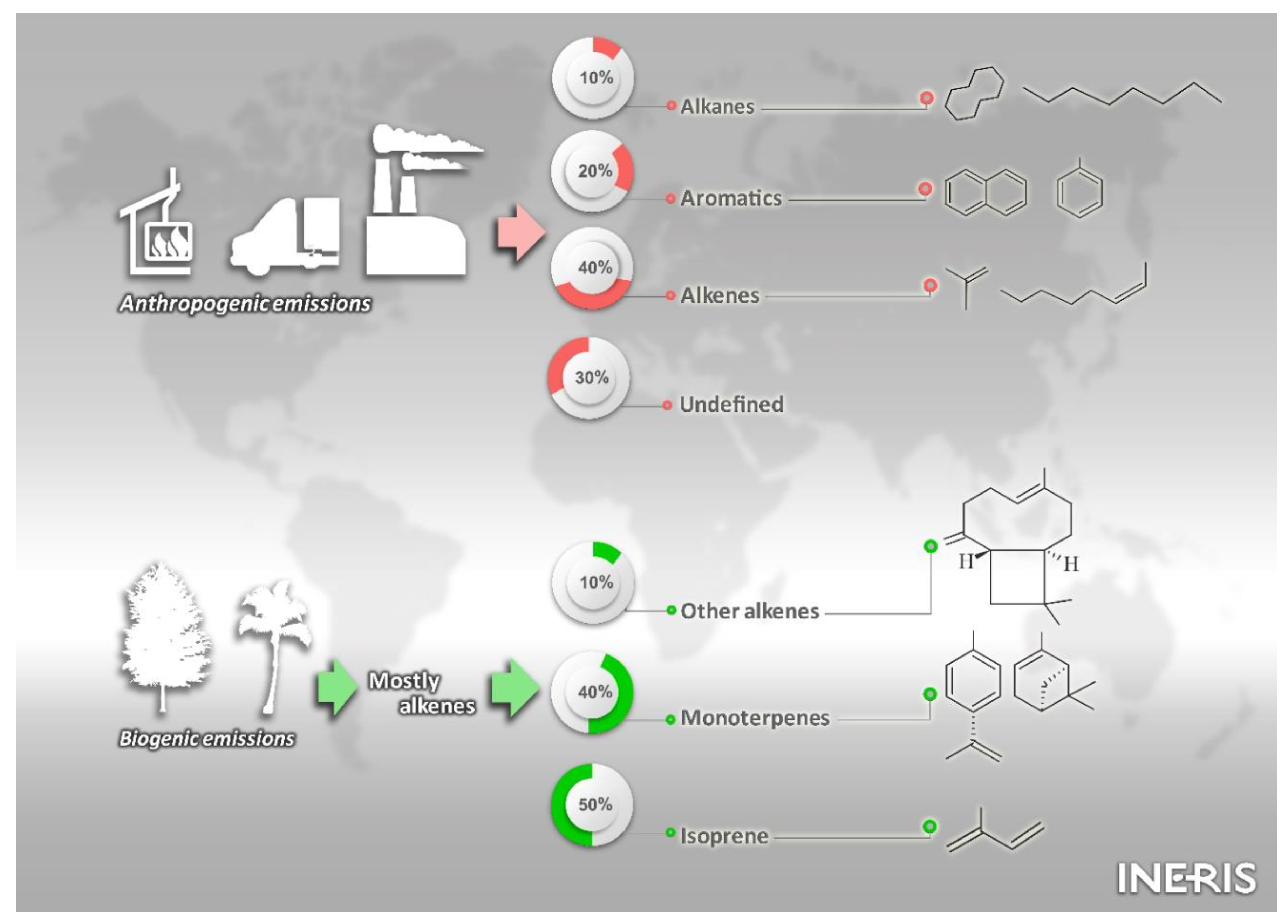
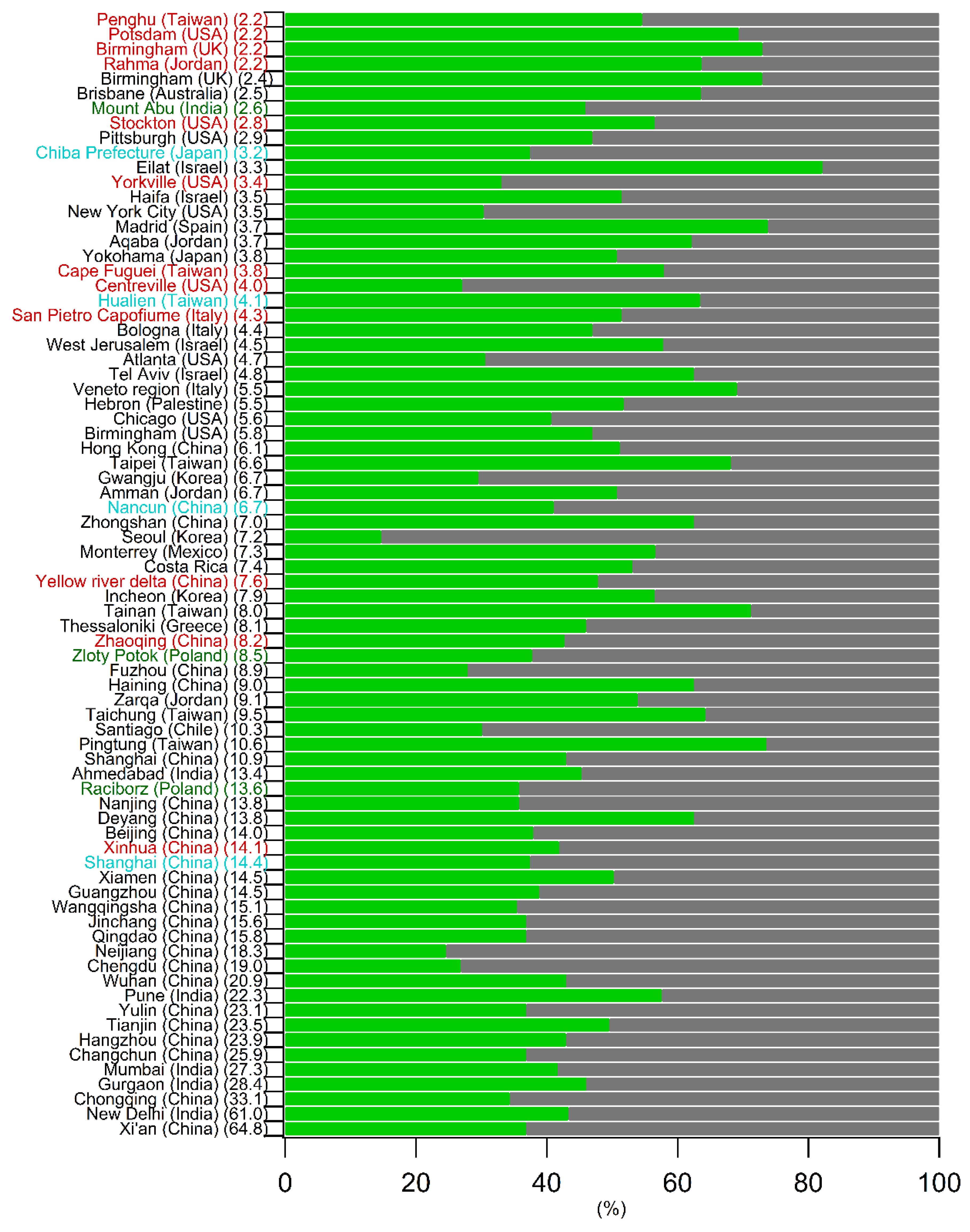
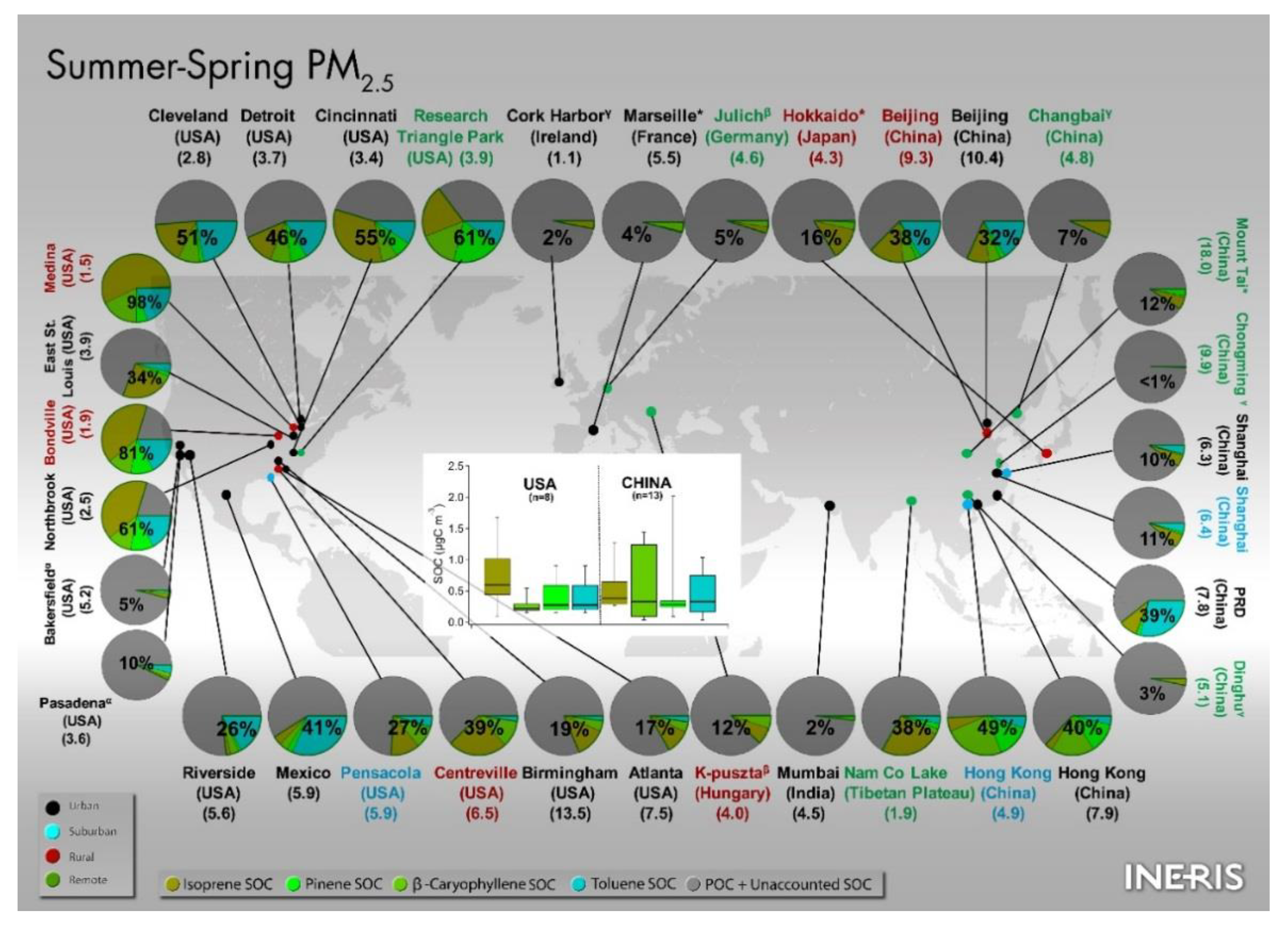
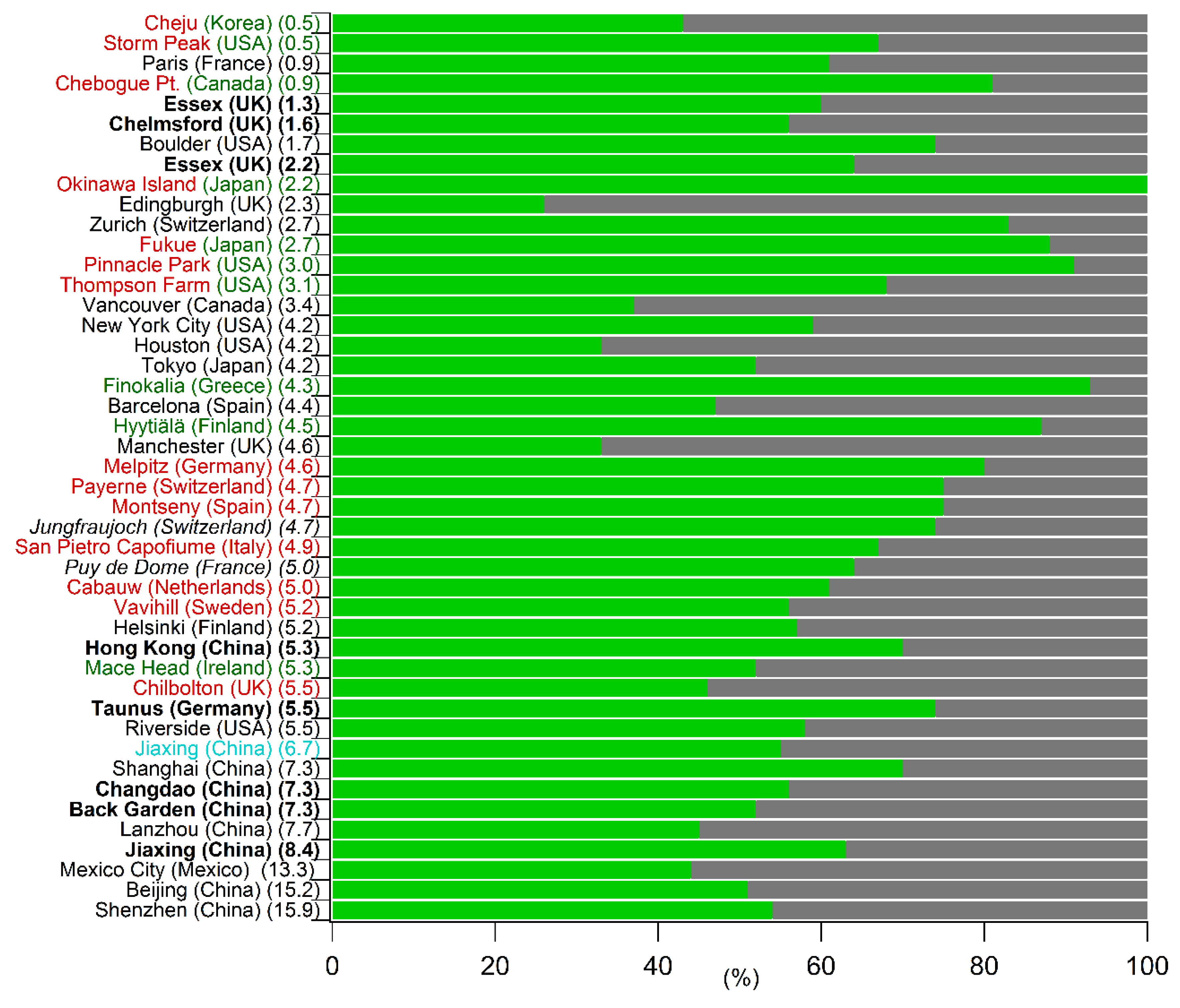
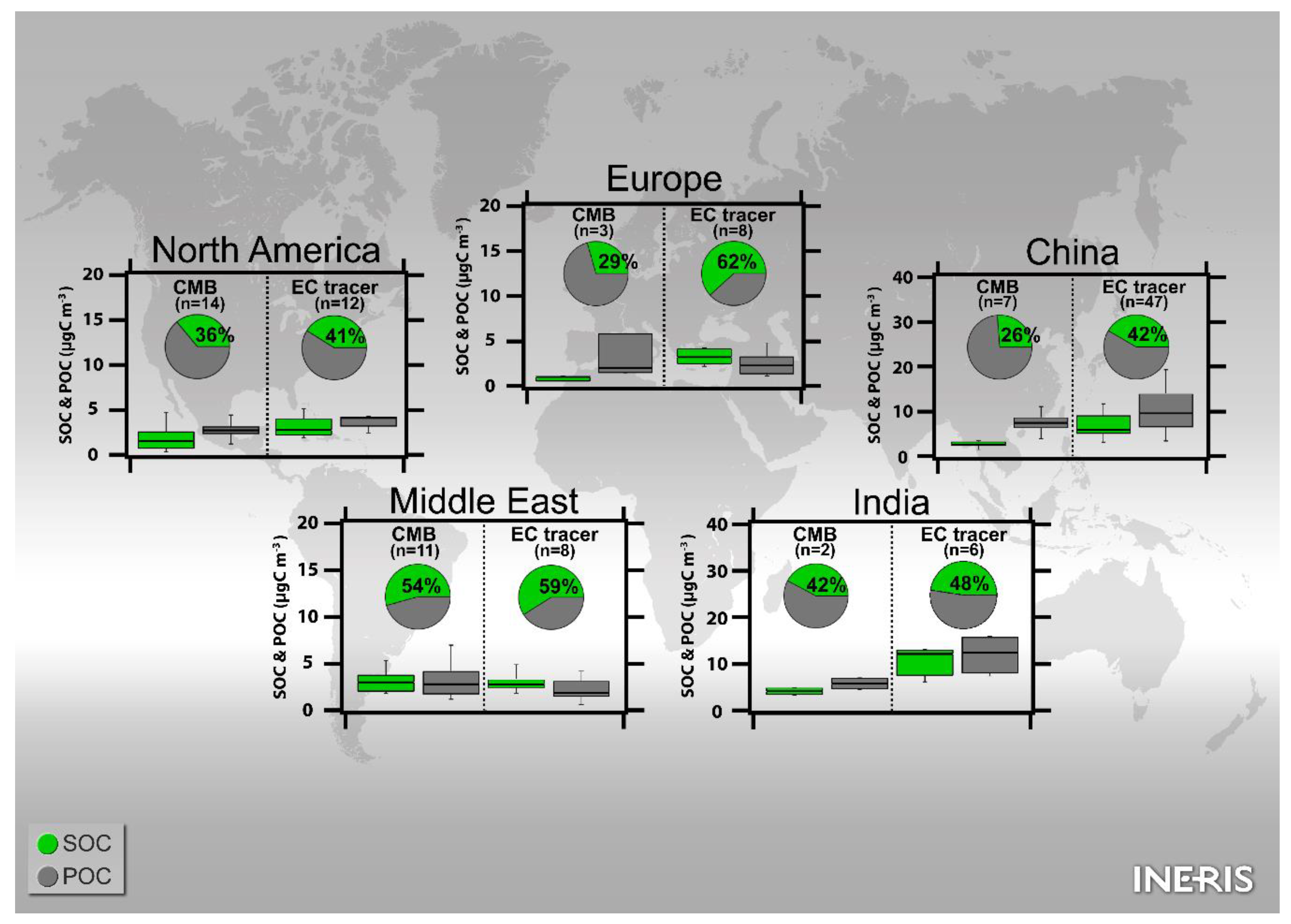
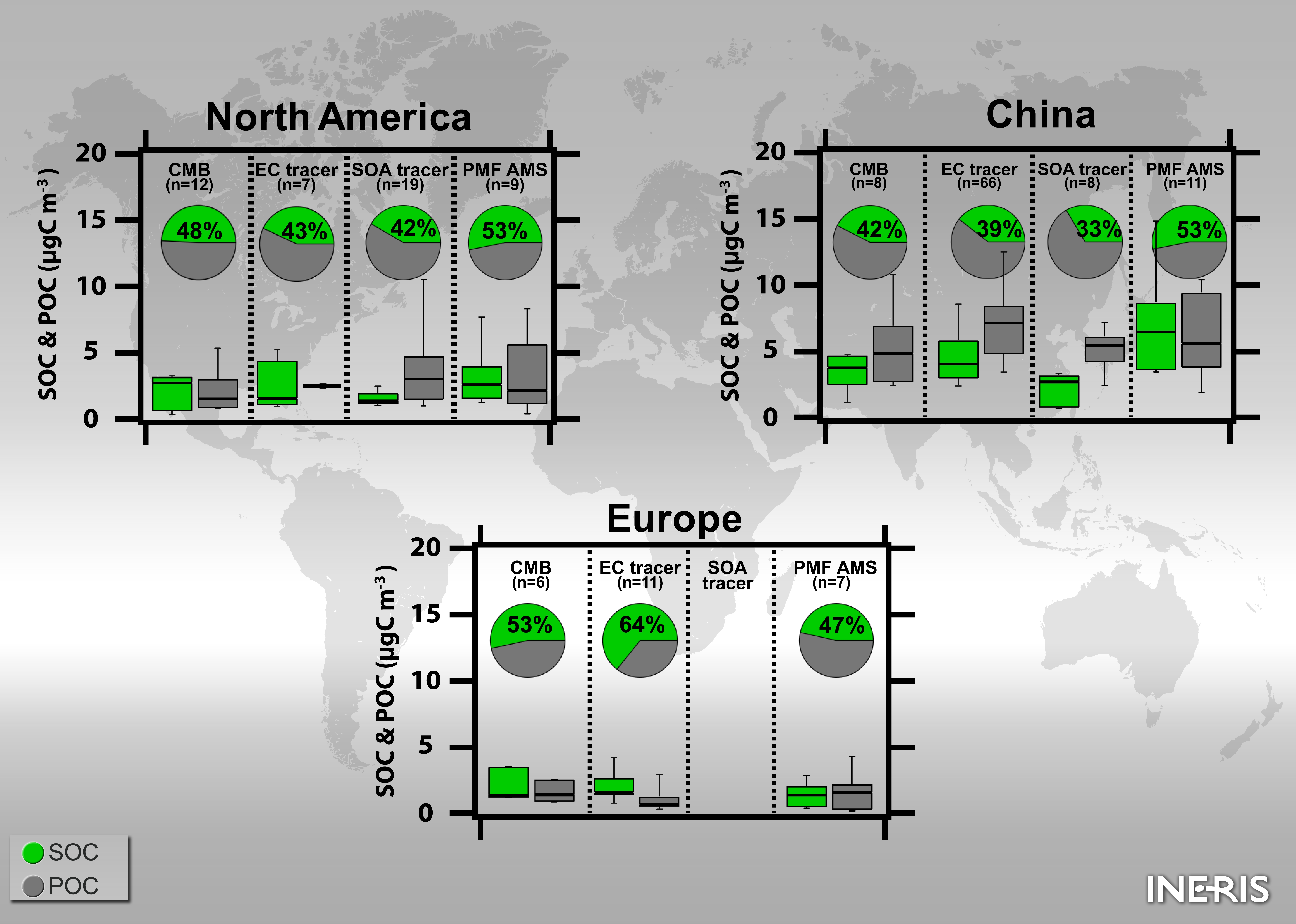
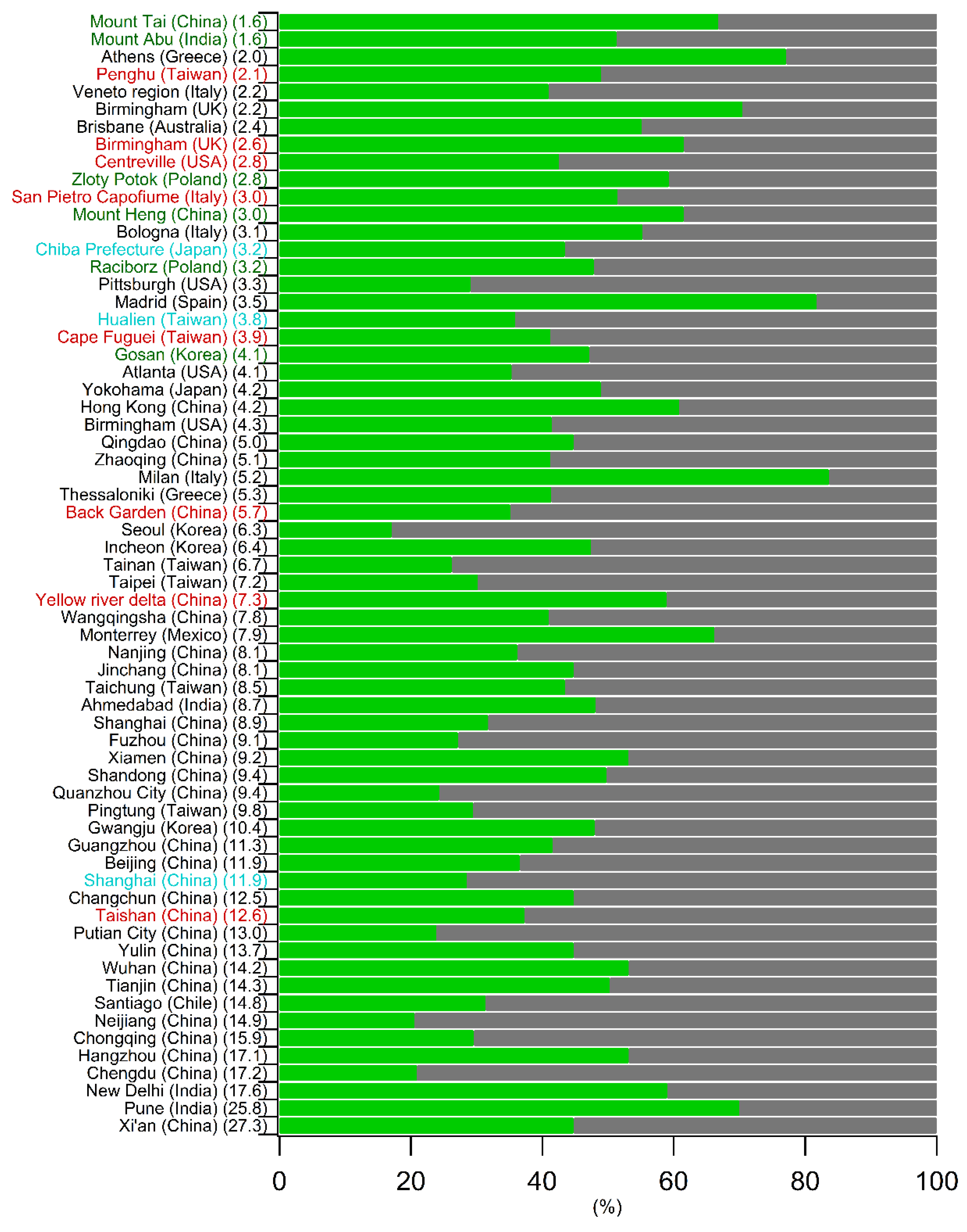
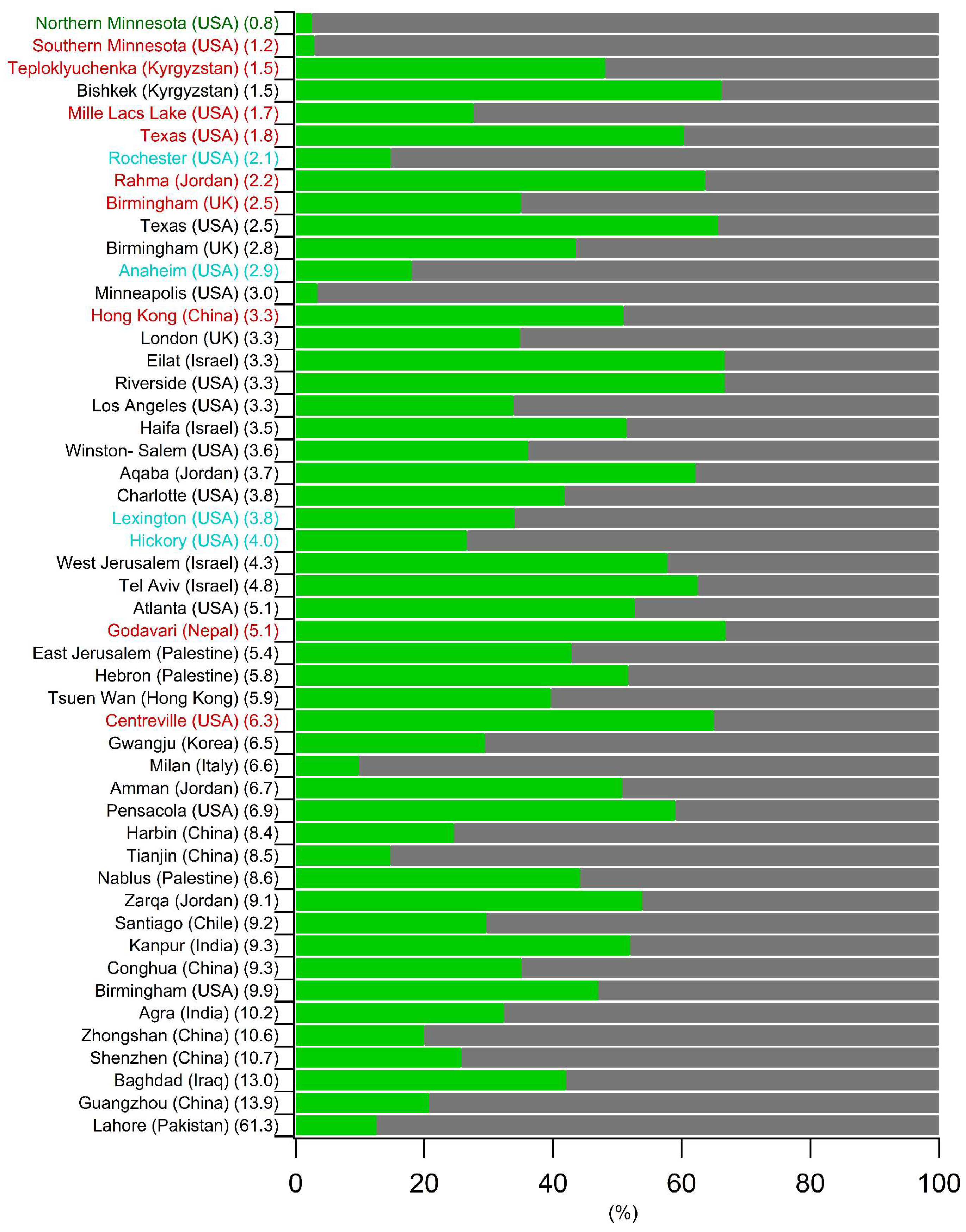
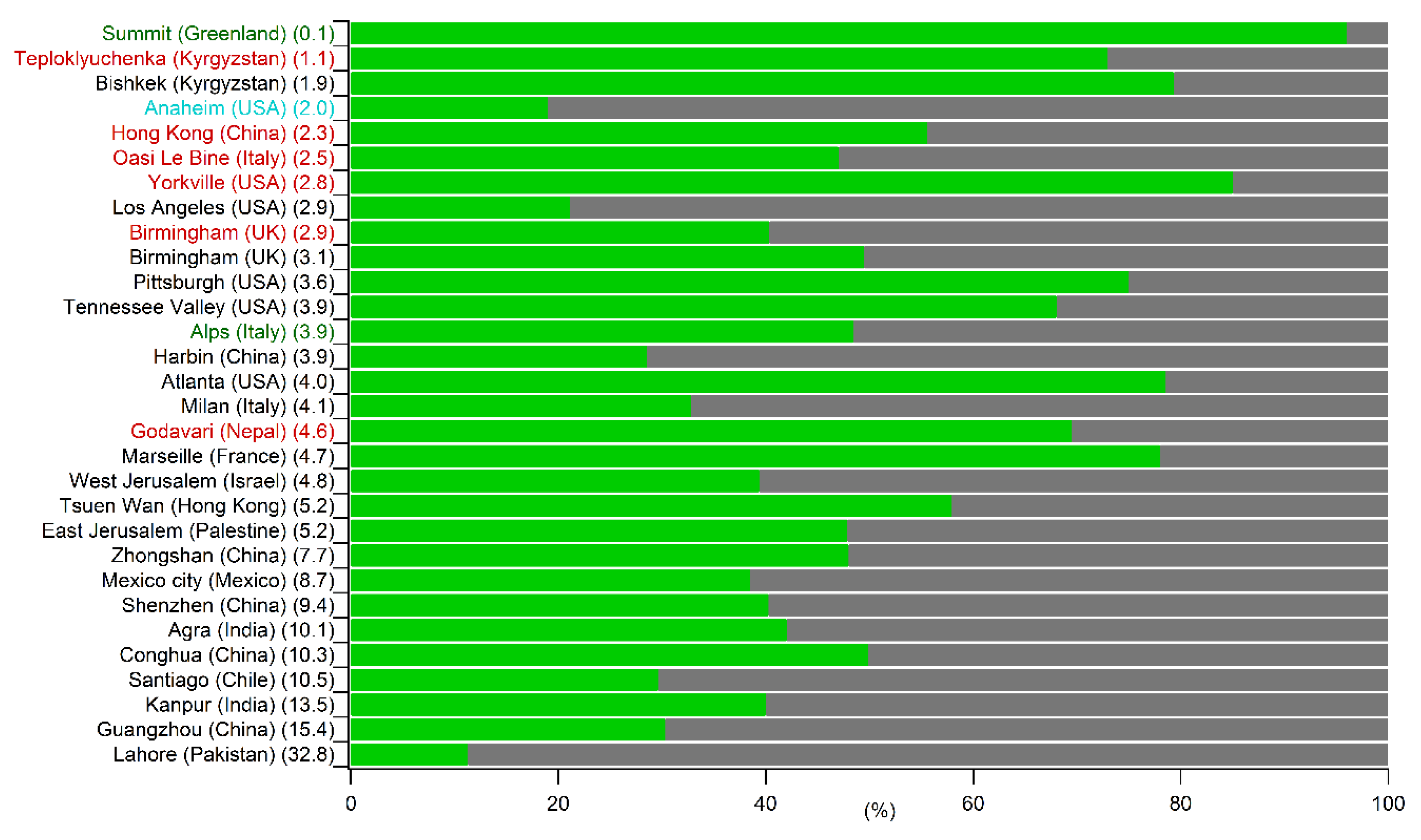
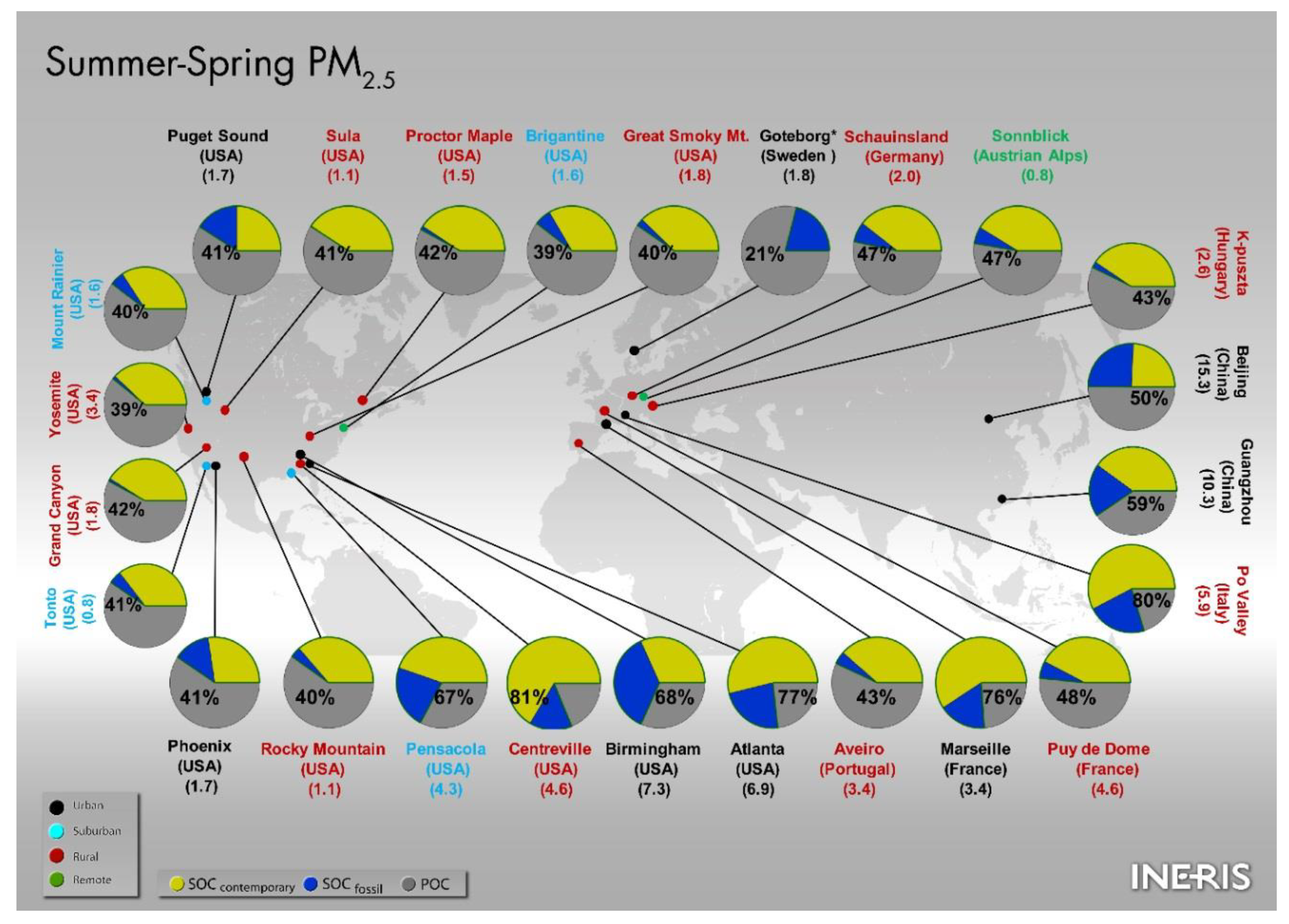
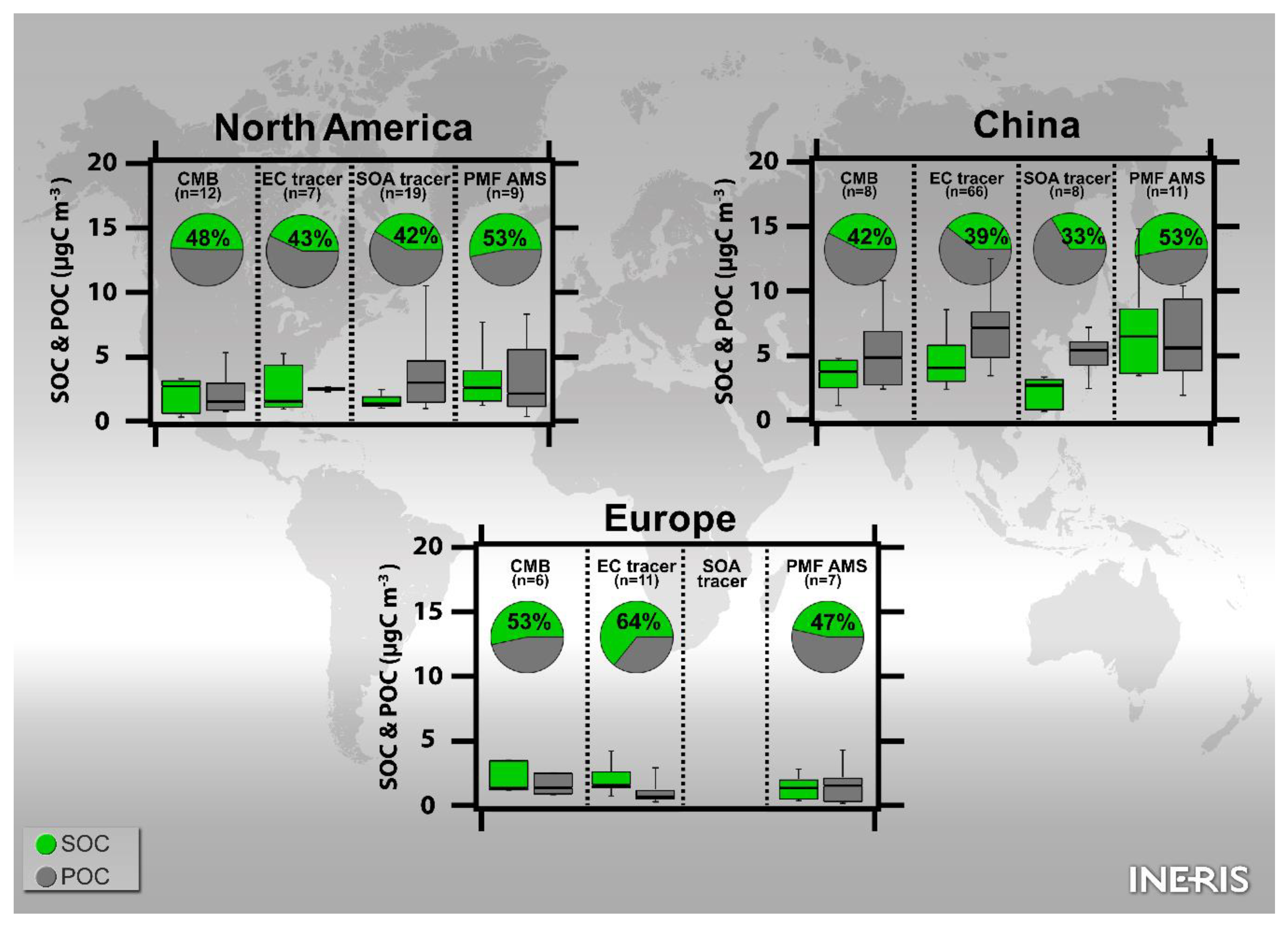
Locations	Sampling Periods	Methodologies				Main Conclusions	References
		EC-Tracer	CMB	SOA-Tracer	PMF
Pittsburgh, Pennsylvania (USA)	Annual (July 2001–July 2002)	X	X			Good agreement (r2 = 0.71, slope = 0.75). Better in summer (r2 = 0.81, slope = 0.91) than in winter (r2 = 0.45, slope = 0.75).	[207]
London, Birmingham, Birmingham (UK) *	Summer (June 2010–August 2010)	X	X			SOC estimates were in broad agreement (urban sites, r2 = 0.70–0.92, slope = 0.80–0.92; rural site, r2 = 0.69–0.92, slope = 0.73–0.88).	[124]
Atlanta, Birmingham, Centreville, Yorkville (USA)	Annual (January 2000–December 2002)	X	X		√ 1	Lower SOC estimates using PMF. Good correlation between SOC estimates using CMB and EC tracer method (CMB vs. EC, r = 0.67–0.84; CMB vs. PMF, r = 0.58–0.74; EC vs. PMF, r = 0.40–0.78). Comparable SOC levels (CMB vs. EC) at urban sites while at rural sites, larger SOC levels estimated using CMB.	[205]
Atlanta (USA)	Summer/Winter (February 1999–December 2007)	X	X		√ 1	Higher SOC estimates using CMB especially in winter. CMB vs. EC vs. PMF: summer: 2.0 ± 0.9 vs. 1.5 ± 1.4 vs. 1.4 ± 0.8 µg m−3; winter 1.8 ± 1.0 vs. 0.8 ± 2.0 vs. 0.9 ± 0.9 µg m−3. The highest uncertainty was obtained using the EC tracer method. The PMF uncertainties were significantly higher than the uncertainties in the CMB method.	[93]
Pittsburgh (USA)	Annual (July 2001–August 2002)	X	X		√√√ 1,2	All methods (EC tracer, CMB, PMF-filter and PMF-AMS) provided the same seasonal pattern with more SOA in summer than in winter. Summer, EC tracer vs. other approaches: 55–70% vs. 30–40% SOC in PM2.5 OC; winter, CMB vs. other approaches: 50 vs. 10% SOC in PM2.5 OC. PMF-filter vs. CMB: Non-winter: r2 = 0.55, slope = 0.72; in winter, poor correlation and low slope.	[14]
Riverside (USA)	Summer (July 2005–August 2005)	X	X		√√	SOA estimates were consistent for all the methods. Diurnal cycles of SOA/OA ratios were similar with maximum ratios observed during the early afternoon. However, the EC-tracer method apportioned SOA slightly differently throughout the evening/night.	[1]
Birmingham, Centreville, Atlanta (USA)	Spring/Summer (August 2003–August 2005)	X		X		For Atlanta, SOC estimates were similar (EC vs. SOA tracer: spring: 1.4 vs. 1.3 µg m−3; summer: 1.2 vs. 1.4 µg m−3). For Birmingham and Centreville, the differences were significantly larger (on average, 1.8 vs. 2.8 µg m−3; 1.2 vs. 2.7 µg m−3, respectively).	[38]
Wangqingsha, Pearl River Delta (China)	Summer (August 2008–September 2008), Fall–Winter (November 2008–December 2008)	X		X		Good agreement in summer (r = 0.57, slope = 0.91, EC vs. SOA tracer SOC: 3.2 vs. 3.1 µg m−3) and better than in fall–winter (EC vs. SOA tracer SOC: 6.7 vs. 2.0 µg m−3). The minimum OC/EC ratio could be not representative of (OC/EC)p in winter season (biomass burning impacted). In fall–winter, other SOA precursors (“non-traditional” SOA) were probably significant but not considered in the SOA tracer method.	[178]
Marseille (France)	Summer (June 2008–July 2008)		X	X		Both methods followed different temporal trends (only biogenic SOC was considered for the SOA tracer method) (r2 = 0.18). CMB vs. SOA tracer: 2.1–8.5 vs. 0.0–0.6 µg m−3.	[41]
Hong Kong, (China)	Summer (July 2006–August 2006)		X	X	√ 1,2	SOC estimates showed very similar time evolutions throughout the sampling period. The average SOC from CMB, PMF-filter and SOA tracer method were: 7.8, 6.8 and 5.0 µg m−3 during high pollution episodes (regional transport) and 1.2, 0.7 and 0.5 µg m−3 under the influence of local emissions (local days).	[40]
Detroit, Cincinnati, East St. Louis, Northbrook, Bondville (USA)	Annual (March 2004–February 2005)			X	√ 2	SOA estimates were highly consistent except for few months with high secondary contributions (r2 = 0.76, slope = 1.01). Underestimation by PMF when the secondary contributions were very low.	[26]
Shanghai (China) 2 sites: 1 urban + 1 suburban	Winter (January 2010, January 2011)/Spring (April 2010–May 2010)/Summer (July 2010)/Autumn (October 2010–November 2010)	X		X	√ 1,2	SOA contributions might be underestimated with the SOA tracer method (only terpenes and aromatic compounds considered). EC vs. SOA: fall–winter: 2.8–8.8 vs. 0.1–0.4 µg m−3; spring–summer 1.5–2.2 vs. 0. 1–0.6 µg m−3. PMF (2.1–2.8 µg m−3) with no variation: a large part of the SOC was associated with nitrate and sulfate but not with the measured SOA tracers. SOA tracer and PMF-filter SOC estimates were significantly correlated (r2 = 0.68). As commercial standards for many of the tracers are not available, large uncertainty in the quantification of the SOA tracers.	[179]
Atlanta (USA)	Summer (July 2001–August 2001)/Winter (January 2002)		X		√ 1	Good correlation between SOC estimates (CMB vs. PM, r2 = 0.43–0.50, slope = 3.2–7.4). Larger SOC estimates using CMB may be due to the unresolved primary OC that would attribute to the CMB (high bias) and the SOA from the resolved primary sources that have not been included in the PMF SOA (low bias).	[303]
Hong Kong (China) 10 sites: 9 urbans + 1 traffic	1998–2002	X			√ 1	The SOC estimates by the EC tracer method were consistently higher than PMF method. Overestimation by 70–212% for the summer samples and by 4–43% for the winter samples. The overestimation by the EC tracer method resulted from the inability of obtaining a single OC/EC ratio that represented a mixture of primary sources varying in time and space.	[98]
Mexico City (Mexico)	Spring (March 2006)		X		√√	Better agreement using CMB estimates corrected from PMF LOA factor (local low nitrogen OA): 49% (PM2.5 OC) vs. 46% (PM1 OC); r2 = 0.40, slope = 1.01.	[348]
Guangzhou (China)	Summer (July 2006)	X			√√	Good correlation between SOC and OOA from PMF (r2 = 0.60) but low regression slope (0.31) indicating that there was a substantial amount of noncarbon elements (e.g., O, N) in OOA.	[168]
Jiaxing, Yangtze River Delta (China)	Summer (July 2015)/Winter (December 2015)	X			√√	Good agreement in summer with similar time trends (PMF vs. EC tracer: 7.2 vs. 6.8 µg m−3). In winter, strong biomass burning events led to overestimate SOA using the EC tracer method (3.9 vs. 7.0 µg m−3).	[349]
Beijing (China)	Fall (November 2013)	X			√√	SOC estimates obtained using EC tracer method were consistent with those from PMF (r2 = 0.69) with very similar concentration levels.	[153]

Used methods: X; Filter-based PMF: √; PMF-AMS: √√; Filter-based PMF and PMF-AMS: √√√; ¹ SOC based on sulfate and nitrate factors; ² SOC factors based on SOA molecular markers; * underlined: rural sites; italic: suburban sites; normal: urban sites.

).

4.1. EC-Tracer vs. CMB

A direct comparison between CMB and EC tracer methods has been reported in at least six studies [1,14,93,124,205,207] (Table 1).

Overall, in terms of both correlations and absolute concentrations, a good agreement between both methodologies has been observed in summer while the differences in winter were significantly larger. As explained before (Section 3.1.2), the determination of [OC/EC]_p in the EC tracer method might be challenging in winter due to the significant influence of local primary emissions. Contrarily, as observed in Pittsburgh (US), under the influence of regional air masses with high SOA background concentration levels, [OC/EC]_p and/or the intercept used in the EC-tracer method may be overestimated leading to an underestimation of the SOC concentrations [14,207]. The impact of the determination of [OC/EC]_p has also been observed for the study of the SOC diurnal cycles in Riverside (CA, US). The reported diurnal cycles were similar using both EC tracer and CMB methodologies (and PMF too) but slightly higher SOA/OA ratios have been observed throughout the evening/night using the EC-tracer method. This probably resulted from lower [OC/EC]_p estimated during the night due to reduced diesel traffic at that time [1]. Overall, the CMB approach seemed to overestimate SOC by comparison to the EC tracer method and again especially in cold period. This overestimation could be due to the significant contributions to OC of unknown and/or unresolved primary sources (e.g., cooking activities and natural gas combustion) then accounted as SOC [205] (see Section 3.2.2). Besides, SOC estimates seemed comparable at urban sites while larger values from CMB were observed at rural sites [205]. Again, the estimation of [OC/EC]_p is quite challenging especially in remote locations which are far from primary sources (see Section 3.1.2). Finally, higher uncertainties have been noticed using the EC tracer method and can be explained by the different approaches used for the estimation of [OC/EC]_p [1,93].

4.2. SOA-Tracer vs. Other Methodologies (EC-Tracer, CMB and PMF-Filter)

A comparison of SOC evaluated data using the SOA tracer method with those obtained using other methodologies such as the EC tracer method, CMB and PMF has been reported in few studies [26,38,40,41,178,179] (Table 1).

Results obtained using the SOA tracer approach agreed well with data reported from the above other methodologies. However, the SOA tracer method tended to underestimate the SOC concentrations. As explained before (Section 3.3.2), the number of SOA tracers and so, of SOA precursors, considered in the method is limited. This is especially true for anthropogenic SOA precursors (i.e., only toluene SOA is considered) explaining that the agreement observed was better in summer [38,178], with a stronger biogenic SOA impact, than in the fall–winter period [178,179]. SOA derived from biomass burning in such periods could be significant but is not considered in the “traditional” SOA tracer method. Besides, the accuracy of both CMB and EC tracer methodologies, could be affected by local primary sources in winter (see Section 3.1.2, Section 3.2.2 and Section 4.1). However, the agreement between the SOA tracer method with CMB could also be low even in summer when only biogenic SOA tracers are considered, highlighting the importance of anthropogenic SOA precursors even in warm period [40,41,179]. The comparisons made with PMF-filter were quite consistent [26]. It is also worth to note that when the secondary contributions were very low, the PMF-filter method underestimated the SOC concentrations, by comparison with the SOA tracer. This may be due to the non-linearity of the yield curve or to errors introduced by PMF-filter because of the error structure of data at these very low levels [26]. Finally, large uncertainties in the SOA tracer method could be linked to the fact that the quantification of the SOA markers was not achieved with the use of authentic standards [179] (Section 3.3.2).

4.3. PMF vs. Other Methodologies (EC-Tracer, CMB)

There are several examples in the literature where the PMF-filter or PMF-AMS [1,14,26,40,93,98,153,168,179,205,303,348,349] methodologies have been compared with the CMB and/or EC tracer methods (Table 1).

A good agreement between PMF, for both PMF-filter and PMF-AMS, and the other methodologies, has been usually observed with significant correlations and similar SOC estimates. As explained before, both CMB and EC tracer methods tended to overestimate SOC, notably in the winter period, due to the inherent limitations of both methodologies when the sampling site is locally influenced by primary emissions [14,93,98,179,205,303,349] (see Section 3.1.2, Section 3.2.2 and Section 4.1).

The impact of local sources has been highlighted by Aiken et al. (2009) who observed, in spring in Mexico, a better agreement between CMB and PMF-AMS after subtracting the local low nitrogen OA fraction (LOA) from the non-apportioned OC, assumed to be SOC, initially obtained with CMB. In addition, the difference between PMF-AMS and the EC tracer method could also be significant even in summer when a substantial amount of non-carbon elements (i.e., O, N) were probably included in the OOA [168]. However, the good agreement between PMF-AMS and the other methodologies was supported by the fact that nice correlations (r² = 0.9) and regression slopes (0.8–0.9) were usually obtained between POC and HOA (in summer) [168,307,348].

SOC estimated from the PMF-filter approach was generally lower than that from the CMB or EC tracer methodologies [14,98,205]. PMF could over-attribute OC to certain factors because the model fits the measured OC while CMB only fits the molecular marker data. This occurred if markers for some important categories of OC (typically SOC ones) were not included in the PMF model [14]. Without the use of SOA markers, SOC was apportioned based on the OC content of the nitrate and sulfate factors (see Section 3.4.3) and the results obtained could not provide further information on SOC because of the co-linearity of OC sources [93]. As mentioned before for the SOA tracer method (Section 3.3.2), the identification of new molecular markers from other SOA precursors is strongly needed and would allow a better description of the SOC associated with nitrate and sulfate factors [179].

Finally, the different SOC apportionment approaches provide consistent results and they can achieve the same conclusions especially in the warm period. A good SOC apportionment may be more difficult to achieve when the influence of local (anthropogenic) emissions, like in the cold period, is significant (EC tracer method and CMB) or due to the lack of SOA molecular markers to account SOA from, notably, anthropogenic precursors and/or sources (SOA tracer method and PMF-filter).

5. Comparison Based on the Overall Picture Obtained from the Review of Recent Studies

The above discussions show that results obtained using different SOC apportionment methodologies are comparable under certain conditions. Thus, a comparison of the SOC estimates obtained worldwide, and reviewed before, is proposed in this section. To get comparable results, only urban and suburban locations are considered and both, annual and spring–summer SOC estimates are discussed.

5.1. Comparison of the Annual SOC Estimates Obtained Worldwide

A comparison of annual SOC estimates obtained in North America, Europe, the Middle East, India and China using CMB and EC tracer method is presented on Figure 9 (data from Tables SA2 and SB2). Results from other methodologies are not included due to the lack of data points on an annual scale.

Overall, SOC estimates evaluated using the EC tracer method are always larger than the ones obtained with CMB whatever the geographical region considered. In North America, the agreement observed is quite good, but the differences are particularly notable for Europe and China where a factor of about two, in terms of both contributions and concentrations, between both methodologies can be observed. Similarly, in India, a factor of two can also be noted but only for SOC concentrations. Both estimated SOC contributions are quite similar in this case. Previous discussions have already accentuated the fact that the selection of [OC/EC]_p is quite challenging in cold period (fall–winter) under the influence of local primary sources (notably biomass burning) leading to an overestimation of SOC (see Section 3.1.2 and Section 4). This is particularly true in Europe, China and India where biomass burning for residential heating, and to a lesser extent, for cooking purposes, is one of the major sources of OA in winter [30,350,351,352,353]. However, this is also true for North America but the factor of two difference is not observed. This is probably because the sites/locations where the CMB and EC tracer studies have been performed are not necessarily the same and are geographically distant (Figures SA1 and SB1, SM). Interestingly, the SOC estimates in the Middle East using CMB and EC tracer method are very similar. The stable climate and meteorological conditions through the year with no proper heating period explain such observations with low bias between both methodologies.

Despite the limitations of both methodologies (see Section 3.1.2, Section 3.2.2 and Section 4), clear patterns can be observed with annual SOC and POC concentration levels, comparable in India and China and twice higher than the ones estimated in the other regions of the world. These results agree with modelling evaluations in terms of both annual SOA concentration levels and world distribution [354]. They also highlight the significant influence of anthropogenic SOA in the developing countries [145,354]. It seems more difficult to conclude in terms of SOC contributions due to the inherent limitations of both methodologies especially when the cold period is also considered. A probably better overview can be made based on spring–summer SOC estimates only, as presented in the next section.

5.2. Comparison of the Spring–Summer SOC Estimates Obtained Worldwide

The comparison of SOC estimates obtained for the spring–summer period in North America, Europe and China using CMB, EC tracer, SOA tracer and PMF-AMS methodologies is presented on Figure 10 (data from Tables SA3, SB3, SC3 and SD2). The results from the SOA tracer method are not included for Europe to avoid any kind of false representation because only biogenic SOC has been accounted in the reviewed studies. Results from ¹⁴C measurements are also not included because they arise from other methodologies such as EC tracer or CMB.

When focusing on the warm period, a good agreement can be seen between all methodologies for both SOC contributions and average SOC concentrations. However, the SOA tracer method tends to underestimate the SOC estimates and it is particularly obvious for China. The rapid urbanization and industrialization in China have led to high emission of anthropogenic SOA precursors [145]. However, and as detailed before (Section 3.3.2 and Section 4.2), only one anthropogenic marker (DHOPA) from toluene photooxidation is accounted for the SOA tracer method to estimate the SOA from anthropogenic sources. SOC from the oxidation of many other VOCs and SVOC/IVOCs (i.e., alkanes, PAHs, furans, phenolic compounds) is not considered using such methodology. It is true that biogenic emissions of isoprenoids (including both isoprene and monoterpenes) are significantly larger than the emissions of anthropogenic VOCs in China during daytime in summer [355]. Nevertheless, several studies have also shown a high regional background of anthropogenic VOCs in summer that could lead to significant secondary SOA formation [179,198] explaining the observed SOC underestimation using the SOA tracer method. Besides, biogenic emissions, including SOA precursors such as isoprene and monoterpenes, significantly impact the organic loading during summer in North America [44,219,220,293,294,295,296] (Section 3.2.3.1, Section 3.3.3.1 and Section 3.5.3.1). As seen before, the biogenic SOA fraction is well documented in the SOA tracer method (see Section 3.3) explaining the comparable SOC estimates obtained with the other methodologies for North America.

Finally, the SOC contributions to PM_2.5 or PM₁ OC in the spring–summer period are comparable in all the considered regions with values ranging from 39% to 64% (excluding the SOA tracer method for China). Average spring–summer SOC concentration ranges are similar in North America and Europe (1–3 µgC m⁻³) and are significantly higher in China (4–6 µgC m⁻³). The relatively good consistency between the different methodologies in North America, for both SOC concentration levels and contributions, may suggest that forest fire events, which are usually episodic in summer, are not a major contributor to SOA, although they could play an important role on the PM concentration levels [346,347]. Biogenic SOA should dominate in such seasons. It is also worth to note the wide range of SOC concentrations observed in China notably from the PMF-AMS results. The country experiences recurrent severe haze pollution events even in summer time, with fine PM reaching very high concentration levels across many cities [145,356] and SOA is a significant contributor to such PM concentrations [145,148]. Thus, these specific events, especially characterized using AMS/ACSM instrumentation, could explain, to a certain extent, the observed variability of SOC concentrations in China.

6. Conclusions and Future Implications

This review has discussed the results reported on SOC estimates obtained by different methodologies reported in the literature. Although the SOC estimates are method dependent, the results reviewed here confirm that SOC constitutes a significant fraction of OC.

The different methodologies to apportion SOC are subject to a certain number of uncertainties but they provide quite consistent results especially in the warm period (spring–summer). Some discrepancies can be observed due to their inherent limitations when the cold period is considered. In such cases, the selection of the appropriate methodology should be done very carefully because each approach has its own advantages and disadvantages and the use of a single approach can cause severe misinterpretation. Thus, this review hardily recommends the use of a combination of different SOC estimation methodologies to apportion the SOC concentrations/contributions in order to get the highest level of confidence in the results obtained. This further suggests that a combination of approaches could enhance the understanding about subtle differences existing in OA contents from different measurements.

As it requires only the determination of the concentrations of EC and OC and generally provides good SOC estimates, the EC tracer method is clearly the easiest methodology to use and should be applied as a base one. However, it is also strongly limited in winter due to the difficulty to estimate primary OC-to-EC ratio without any ambiguity.

CMB also provides SOC concentrations and contributions in good agreement with the other approaches. The lack of emission profiles for uncommon and thus un-apportioned sources inducing an overestimation of SOC, is the principal limitation of this methodology. This is especially the case when the sampling site is strongly affected by local emission sources. Thus, CMB is probably one of the most difficult approaches to apply, as source profiles for SOC do not exist and this may lead to an over/underestimation depending on the conditions. Therefore, CMB is not the first recommended approach. The current development of emission profile databases, such as SPECIATE or SPECIEUROPE, is of great value to get the appropriate input to the CMB model for each case study and can clearly improve the evaluation of SOC using such approaches [357,358].

In combination with such methodologies, the use of radiocarbon measurements (¹⁴C) may provide detailed information on the SOC origins and can be helpful to improve the understanding of the atmospheric involved processes. Nevertheless, the main limitations are related to the analytical costs and the amount of material required. Thus, this methodology is difficult to implement routinely. Such a method should be applied only on short-term campaign datasets in combination with other approaches (EC tracer or CMB) to refine and improve the SOC estimates.

Similarly, PMF-AMS/ACSM provides a good estimation of SOC, together with additional information about the SOA oxidation state and/or the volatility range. Detailed analyses can highlight additional sub-SOA fractions such as IEPOX-SOA or marine SOA [298,317,318,319,320]. More sub-SOA factors are then expected but they are difficult to be resolved due to the non-specific nature of the obtained mass fragments.

Only a detailed chemical characterization at the molecular level and the use of key species, i.e., molecular markers, can allow a definitive link between SOC content and SOA origins to be obtained. Both the SOA tracer and PMF-filter methods have been shown to be in good agreement with the other SOC apportionment methodologies, especially in the warm period in the case of the SOA tracer method. In such periods, the larger biogenic emission rates and biogenic SOA fraction is precisely considered in the SOA tracer method. This is not true for anthropogenic SOA precursors, explaining the underestimation often observed for other periods of the year, especially in winter when the SOA derived from biomass burning could be substantial but not considered in the “traditional” SOA tracer method. The lack of markers for several SOA sources or SOA precursors, notably to account for anthropogenic SOA, together with the SOA/SOC mass ratio data, are probably the main limitations of the SOA tracer method. Large uncertainties in this method could be linked to the fact that the quantification of SOA markers is not uniformly achieved (same surrogate compounds used, and/or no authentic standards are often used). Thus, the SOA tracer method is, in the current state of research, fully applicable in the case of biogenic influenced sampling sites but probably not recommended in the winter period or when the locations are highly impacted by anthropogenic activities. When SOA molecular markers are used in the PMF approach, the primary/secondary OA split depends on the species used. As PMF analysis requires a larger number of samples and molecular markers to get a statistically robust and meaningful solution, an expensive and exhaustive sample analysis work is required. Finally, further works are needed to identify SOA molecular markers from VOC and SVOC/IVOCS precursors and notably anthropogenic ones including markers for organosulfates, organonitrates, and multi-phase (aqueous) processes. Additionally, an experimental evaluation of the atmospheric stability of the main molecular markers is still necessary [42].

The full distinction and comprehension of OA sources are still difficult to achieve due to the complexity and the variability of the processes involved. In comparison to AMS/ACSM, the recent development of new instruments provides an online aerosol chemical characterization at the molecular level which, combined with PMF analysis, allows a better description of the OA and SOA sources. The shortcomings of low time resolution with filter measurements can be overcome using this kind of instruments to elucidate more information about the chemical processes involved. Such instrumentations include, for instance, TAG-AMS (thermal desorption aerosol gas chromatograph-AMS) [359,360,361], EESI-TOF-MS (extractive electrospray ionization-time of flight-MS) [362,363,364,365,366], or different inlets associated to PTR-MS (proton-transfer reaction-MS) or CIMS (chemical ionization MS) such as FIGAERO (filter inlet for gases and aerosols) [367], CHARON (chemical analysis of aerosol online) or thermo-desorption (TD) systems [37,368,369,370,371], which have been successfully applied to apportion SOC in details. However, these instruments are still costly and only appropriate for short term studies.

In parallel, like in the case of ¹⁴C measurements, several authors have reported the combination of different datasets from several measurement systems to refine the source apportionment of SOA using PMF. Slowik et al. [372] were the first to combine AMS and PTR-MS data measurements, highlighting the capability of PMF to resolve more SOA (OOA) factors and improving the interpretations of their sources and photochemical processes [333,372]. This kind of approach has been explored in other studies, with the combination of AMS or ACSM data with other measurements, such as ambient and thermally denuded OA spectra (TD-PMF-AMS) [373] or with single particle mass spectrometry [374], by merging high resolution mass spectra of organic and inorganic aerosols from AMS measurements [375,376] or combining offline AMS data and organic markers or ¹⁴C measurements [145,377]. In addition, the combination of PMF-ACSM outputs with inorganic species and black carbon (BC) measurements [378] or ACSM mass spectra with metal concentrations [379], allowed the source apportionment of PM rather than only OA. This further suggests that a combination of approaches could enhance the understanding about subtler differences existing in OA and SOA content by accounting for different measurements.

These improvements in the understanding of SOA origins will facilitate to bridge the existing gap between atmospheric models and field measurements [19,380,381,382].

References

- Docherty, K.S.; Stone, E.A.; Ulbrich, I.M.; DeCarlo, P.F.; Snyder, D.C.; Schauer, J.J.; Peltier, R.E.; Weber, R.J.; Murphy, S.M.; Seinfeld, J.H. Apportionment of primary and secondary organic aerosols in Southern California during the 2005 Study of Organic Aerosols in Riverside (SOAR-1). Environ. Sci. Technol. 2008, 42, 7655–7662. [Google Scholar] [CrossRef] [PubMed]
- Turpin, B.J.; Saxena, P.; Andrews, E. Measuring and simulating particulate organics in the atmosphere: Problems and prospects. Atmos. Environ. 2000, 34, 2983–3013. [Google Scholar] [CrossRef]
- Goldstein, A.H.; Galbally, I.E. Known and unexplored organic constituents in the earth’s atmosphere. Environ. Sci. Technol. 2007, 41, 1514–1521. [Google Scholar] [CrossRef] [PubMed]
- Simoneit, B.R.; Mazurek, M.A. Organic matter of the troposphere—II. For Part I, see Simoneit et al. (1977). Natural background of biogenic lipid matter in aerosols over the rural western united states. Atmos. Environ. 1982, 16, 2139–2159. [Google Scholar] [CrossRef]
- Després, V.; Nowoisky, J.; Klose, M.; Conrad, R.; Andreae, M.; Pöschl, U. Characterization of primary biogenic aerosol particles in urban, rural, and high-alpine air by DNA sequence and restriction fragment analysis of ribosomal RNA genes. Biogeosciences 2007, 4, 1127–1141. [Google Scholar] [CrossRef] [Green Version]
- Jaenicke, R. Abundance of cellular material and proteins in the atmosphere. Science 2005, 308, 73. [Google Scholar] [CrossRef] [PubMed]
- Querol, X.; Viana, M.; Alastuey, A.; Amato, F.; Moreno, T.; Castillo, S.; Pey, J.; de la Rosa, J.; Sánchez de la Campa, A.; Artíñano, B.; et al. Source origin of trace elements in PM from regional background, urban and industrial sites of Spain. Atmos. Environ. 2007, 41, 7219–7231. [Google Scholar] [CrossRef]
- Seinfeld, J.; Pandis, S. Atmospheric Chemistry and Physics; Wiley: Hoboken, NJ, USA, 2006. [Google Scholar]
- Volkamer, R.; Jimenez, J.L.; San Martini, F.; Dzepina, K.; Zhang, Q.; Salcedo, D.; Molina, L.T.; Worsnop, D.R.; Molina, M.J. Secondary organic aerosol formation from anthropogenic air pollution: Rapid and higher than expected. Geophys. Res. Lett. 2006, 33. [Google Scholar] [CrossRef] [Green Version]
- Kanakidou, M.; Seinfeld, J.; Pandis, S.; Barnes, I.; Dentener, F.; Facchini, M.; Dingenen, R.V.; Ervens, B.; Nenes, A.; Nielsen, C. Organic aerosol and global climate modelling: A review. Atmos. Chem. Phys. 2005, 5, 1053–1123. [Google Scholar] [CrossRef]
- Ziemann, P.J.; Atkinson, R. Kinetics, products, and mechanisms of secondary organic aerosol formation. Chem. Soc. Rev. 2012, 41, 6582–6605. [Google Scholar] [CrossRef] [PubMed]
- Zhang, Q.; Jimenez, J.L.; Canagaratna, M.R.; Allan, J.D.; Coe, H.; Ulbrich, I.; Alfarra, M.R.; Takami, A.; Middlebrook, A.M.; Sun, Y.L.; et al. Ubiquity and dominance of oxygenated species in organic aerosols in anthropogenically-influenced Northern Hemisphere midlatitudes. Geophys. Res. Lett. 2007, 34. [Google Scholar] [CrossRef] [Green Version]
- Carlton, A.G.; Wiedinmyer, C.; Kroll, J.H. A review of Secondary Organic Aerosol (SOA) formation from isoprene. Atmos. Chem. Phys. 2009, 9, 4987–5005. [Google Scholar] [CrossRef] [Green Version]
- Shrivastava, M.K.; Subramanian, R.; Rogge, W.F.; Robinson, A.L. Sources of organic aerosol: Positive matrix factorization of molecular marker data and comparison of results from different source apportionment models. Atmos. Environ. 2007, 41, 9353–9369. [Google Scholar] [CrossRef]
- Zhao, Y.; Kreisberg, N.M.; Worton, D.R.; Isaacman, G.; Gentner, D.R.; Chan, A.W.H.; Weber, R.J.; Liu, S.; Day, D.A.; Russell, L.M.; et al. Sources of organic aerosol investigated using organic compounds as tracers measured during CalNex in Bakersfield. J. Geophys. Res.-Atmos. 2013, 118, 2012JD019248. [Google Scholar] [CrossRef]
- Griffin, R.J.; Cocker, D.R.; Flagan, R.C.; Seinfeld, J.H. Organic aerosol formation from the oxidation of biogenic hydrocarbons. J. Geophys. Res. 1999, 104, 3555. [Google Scholar] [CrossRef]
- Hallquist, M.; Wenger, J.; Baltensperger, U.; Rudich, Y.; Simpson, D.; Claeys, M.; Dommen, J.; Donahue, N.; George, C.; Goldstein, A. The formation, properties and impact of secondary organic aerosol: Current and emerging issues. Atmos. Chem. Phys. 2009, 9, 5155–5236. [Google Scholar] [CrossRef] [Green Version]
- Tsigaridis, K.; Daskalakis, N.; Kanakidou, M.; Adams, P.; Artaxo, P.; Bahadur, R.; Balkanski, Y.; Bauer, S.; Bellouin, N.; Benedetti, A. The AeroCom evaluation and intercomparison of organic aerosol in global models. Atmos. Chem. Phys. 2014, 14, 10845–10895. [Google Scholar] [CrossRef]
- Ciarelli, G.; Aksoyoglu, S.; Crippa, M.; Jimenez, J.L.; Nemitz, E.; Sellegri, K.; Äijälä, M.; Carbone, S.; Mohr, C.; O’Dowd, C.; et al. Evaluation of European air quality modelled by CAMx including the volatility basis set scheme. Atmos. Chem. Phys. 2016, 16, 10313–10332. [Google Scholar] [CrossRef]
- Grosjean, D. Particulate carbon in Los Angeles air. Sci. Total Environ. 1984, 32, 133–145. [Google Scholar] [CrossRef]
- Turpin, B.J.; Huntzicker, J.J. Identification of secondary organic aerosol episodes and quantitation of primary and secondary organic aerosol concentrations during SCAQS. Atmos. Environ. 1995, 29, 3527–3544. [Google Scholar] [CrossRef]
- Gray, H.A.; Cass, G.R.; Huntzicker, J.J.; Heyerdahl, E.K.; Rau, J.A. Characteristics of atmospheric organic and elemental carbon particle concentrations in Los Angeles. Environ. Sci. Technol. 1986, 20, 580–589. [Google Scholar] [CrossRef] [PubMed] [Green Version]
- Watson, J.G.; Robinson, N.F.; Chow, J.C.; Henry, R.C.; Kim, B.; Pace, T.; Meyer, E.L.; Nguyen, Q. The USEPA/DRI chemical mass balance receptor model, CMB 7.0. Environ. Softw. 1990, 5, 38–49. [Google Scholar] [CrossRef]
- Paatero, P. Least squares formulation of robust non-negative factor analysis. Chemom. Intell. Lab. Syst. 1997, 37, 23–35. [Google Scholar] [CrossRef]
- Paatero, P.; Tapper, U. Positive matrix factorization: A non-negative factor model with optimal utilization of error estimates of data values. Environmetrics 1994, 5, 111–126. [Google Scholar] [CrossRef]
- Zhang, Y.; Sheesley, R.J.; Schauer, J.J.; Lewandowski, M.; Jaoui, M.; Offenberg, J.H.; Kleindienst, T.E.; Edney, E.O. Source apportionment of primary and secondary organic aerosols using positive matrix factorization (PMF) of molecular markers. Atmos. Environ. 2009, 43, 5567–5574. [Google Scholar] [CrossRef]
- Kleindienst, T.E.; Jaoui, M.; Lewandowski, M.; Offenberg, J.H.; Lewis, C.W.; Bhave, P.V.; Edney, E.O. Estimates of the contributions of biogenic and anthropogenic hydrocarbons to secondary organic aerosol at a southeastern US location. Atmos. Environ. 2007, 41, 8288–8300. [Google Scholar] [CrossRef]
- Liu, J.; Li, J.; Zhang, Y.; Liu, D.; Ding, P.; Shen, C.; Shen, K.; He, Q.; Ding, X.; Wang, X. Source apportionment using radiocarbon and organic tracers for PM2. 5 carbonaceous aerosols in guangzhou, south china: Contrasting local-and regional-scale haze events. Environ. Sci. Technol. 2014, 48, 12002–12011. [Google Scholar] [CrossRef] [PubMed] [Green Version]
- Szidat, S.; Ruff, M.; Perron, N.; Wacker, L.; Synal, H.-A.; Hallquist, M.; Shannigrahi, A.S.; Yttri, K.E.; Dye, C.; Simpson, D. Fossil and non-fossil sources of organic carbon (OC) and elemental carbon (EC) in Göteborg, Sweden. Atmos. Chem. Phys. 2009, 9, 1521–1535. [Google Scholar] [CrossRef] [Green Version]
- Gelencsér, A.; May, B.; Simpson, D.; Sánchez-Ochoa, A.; Kasper-Giebl, A.; Puxbaum, H.; Caseiro, A.; Pio, C.; Legrand, M. Source apportionment of PM2.5 organic aerosol over Europe: Primary/secondary, natural/anthropogenic, and fossil/biogenic origin. J. Geophys. Res. 2007, 112. [Google Scholar] [CrossRef]
- Weber, R.J.; Sullivan, A.P.; Peltier, R.E.; Russell, A.; Yan, B.; Zheng, M.; de Gouw, J.; Warneke, C.; Brock, C.; Holloway, J.S.; et al. A study of secondary organic aerosol formation in the anthropogenic-influenced southeastern United States. J. Geophys. Res.-Atmos. 2007, 112, D13302. [Google Scholar] [CrossRef]
- Blanchard, C.L.; Hidy, G.M.; Tanenbaum, S.; Edgerton, E.; Hartsell, B.; Jansen, J. Carbon in southeastern U.S. aerosol particles: Empirical estimates of secondary organic aerosol formation. Atmos. Environ. 2008, 42, 6710–6720. [Google Scholar] [CrossRef]
- DeCarlo, P.F.; Kimmel, J.R.; Trimborn, A.; Northway, M.J.; Jayne, J.T.; Aiken, A.C.; Gonin, M.; Fuhrer, K.; Horvath, T.; Docherty, K.S. Field-deployable, high-resolution, time-of-flight aerosol mass spectrometer. Anal. Chem. 2006, 78, 8281–8289. [Google Scholar] [CrossRef] [PubMed]
- Jayne, J.T.; Leard, D.C.; Zhang, X.; Davidovits, P.; Smith, K.A.; Kolb, C.E.; Worsnop, D.R. Development of an aerosol mass spectrometer for size and composition analysis of submicron particles. Aerosol Sci. Technol. 2000, 33, 49–70. [Google Scholar] [CrossRef]
- Sun, Y.L.; Zhang, Q.; Schwab, J.J.; Demerjian, K.L.; Chen, W.N.; Bae, M.S.; Hung, H.M.; Hogrefe, O.; Frank, B.; Rattigan, O.V.; et al. Characterization of the sources and processes of organic and inorganic aerosols in New York city with a high-resolution time-of-flight aerosol mass apectrometer. Atmos. Chem. Phys. 2011, 11, 1581–1602. [Google Scholar] [CrossRef]
- Xu, J.; Zhang, Q.; Chen, M.; Ge, X.; Ren, J.; Qin, D. Chemical composition, sources, and processes of urban aerosols during summertime in northwest China: Insights from high-resolution aerosol mass spectrometry. Atmos. Chem. Phys. 2014, 14, 12593–12611. [Google Scholar] [CrossRef]
- Zahardis, J.; Geddes, S.; Petrucci, G.A. Improved understanding of atmospheric organic aerosols via innovations in soft ionization aerosol mass spectrometry. Anal. Chem. 2011, 83, 2409–2415. [Google Scholar] [CrossRef] [PubMed]
- Kleindienst, T.E.; Lewandowski, M.; Offenberg, J.H.; Edney, E.O.; Jaoui, M.; Zheng, M.; Ding, X.; Edgerton, E.S. Contribution of primary and secondary sources to organic aerosol and PM2.5 at SEARCH Network Sites. J. Air Waste Manag. Assoc. 2010, 60, 1388–1399. [Google Scholar] [CrossRef] [PubMed]
- Kourtchev, I.; Warnke, J.; Maenhaut, W.; Hoffmann, T.; Claeys, M. Polar organic marker compounds in PM2.5 aerosol from a mixed forest site in western Germany. Chemosphere 2008, 73, 1308–1314. [Google Scholar] [CrossRef] [PubMed]
- Hu, D.; Bian, Q.; Lau, A.K.H.; Yu, J.Z. Source apportioning of primary and secondary organic carbon in summer PM2.5 in Hong Kong using positive matrix factorization of secondary and primary organic tracer data. J. Geophys. Res.-Atmos. 2010, 115. [Google Scholar] [CrossRef]
- El Haddad, I.; Marchand, N.; Temime-Roussel, B.; Wortham, H.; Piot, C.; Besombes, J.L.; Baduel, C.; Voisin, D.; Armengaud, A.; Jaffrezo, J.L. Insights into the secondary fraction of the organic aerosol in a Mediterranean urban area: Marseille. Atmos. Chem. Phys. 2011, 11, 2059–2079. [Google Scholar] [CrossRef] [Green Version]
- Nozière, B.; Kalberer, M.; Claeys, M.; Allan, J.; D’Anna, B.; Decesari, S.; Finessi, E.; Glasius, M.; Grgić, I.; Hamilton, J.F.; et al. The molecular identification of organic compounds in the atmosphere: State of the art and challenges. Chem. Rev. 2015. [Google Scholar] [CrossRef] [PubMed] [Green Version]
- Tsigaridis, K.; Kanakidou, M. Secondary organic aerosol importance in the future atmosphere. Atmos. Environ. 2007, 41, 4682–4692. [Google Scholar] [CrossRef]
- Guenther, A.; Karl, T.; Harley, P.; Wiedinmyer, C.; Palmer, P.I.; Geron, C. Estimates of global terrestrial isoprene emissions using MEGAN (Model of Emissions of Gases and Aerosols from Nature). Atmos. Chem. Phys. 2006, 6, 3181–3210. [Google Scholar] [CrossRef] [Green Version]
- Guenther, A.; Hewitt, C.N.; Erickson, D.; Fall, R.; Geron, C.; Graedel, T.; Harley, P.; Klinger, L.; Lerdau, M.; McKay, W.A.; et al. A global model of natural volatile organic compound emissions. J. Geophys. Res.-Atmos. 1995, 100, 8873–8892. [Google Scholar] [CrossRef]
- Acosta Navarro, J.C.; Smolander, S.; Struthers, H.; Zorita, E.; Ekman, A.M.; Kaplan, J.; Guenther, A.; Arneth, A.; Riipinen, I. Global emissions of terpenoid VOCs from terrestrial vegetation in the last millennium. J. Geophys. Res.-Atmos. 2014, 119, 6867–6885. [Google Scholar] [CrossRef] [PubMed] [Green Version]
- Kettle, A.J.; Andreae, M.O. Flux of dimethylsulfide from the oceans: A comparison of updated data sets and flux models. J. Geophys. Res.-Atmos. 2000, 105, 26793–26808. [Google Scholar] [CrossRef] [Green Version]
- Kawamura, K.; Sakaguchi, F. Molecular distributions of water soluble dicarboxylic acids in marine aerosols over the Pacific Ocean including tropics. J. Geophys. Res.-Atmos. 1999, 104, 3501–3509. [Google Scholar] [CrossRef] [Green Version]
- Facchini, M.C.; Decesari, S.; Rinaldi, M.; Carbone, C.; Finessi, E.; Mircea, M.; Fuzzi, S.; Moretti, F.; Tagliavini, E.; Ceburnis, D.; et al. Important source of marine secondary organic aerosol from biogenic amines. Environ. Sci. Technol. 2008, 42, 9116–9121. [Google Scholar] [CrossRef] [PubMed]
- Arnold, S.; Spracklen, D.; Williams, J.; Yassaa, N.; Sciare, J.; Bonsang, B.; Gros, V.; Peeken, I.; Lewis, A.; Alvain, S. Evaluation of the global oceanic isoprene source and its impacts on marine organic carbon aerosol. Atmos. Chem. Phys. 2009, 9, 1253–1262. [Google Scholar] [CrossRef] [Green Version]
- Odum, J.R.; Jungkamp, T.P.W.; Griffin, R.J.; Flagan, R.C.; Seinfeld, J.H. The atmospheric aerosol-forming potential of whole gasoline vapor. Science 1997, 276, 96–99. [Google Scholar] [CrossRef] [PubMed]
- Johnson, D.; Utembe, S.; Jenkin, M.; Derwent, R.; Hayman, G.; Alfarra, M.; Coe, H.; McFiggans, G. Simulating regional scale secondary organic aerosol formation during the TORCH 2003 campaign in the southern UK. Atmos. Chem. Phys. 2006, 6, 403–418. [Google Scholar] [CrossRef] [Green Version]
- Kleeman, M.J.; Ying, Q.; Lu, J.; Mysliwiec, M.J.; Griffin, R.J.; Chen, J.; Clegg, S. Source apportionment of secondary organic aerosol during a severe photochemical smog episode. Atmos. Environ. 2007, 41, 576–591. [Google Scholar] [CrossRef]
- Chen, J.; Ying, Q.; Kleeman, M.J. Source apportionment of wintertime secondary organic aerosol during the California regional PM10/PM2.5 air quality study. Atmos. Environ. 2010, 44, 1331–1340. [Google Scholar] [CrossRef]
- Marta, G.V.; Manuel, S. Secondary organic aerosol formation from the oxidation of a mixture of organic gases in a chamber. Air Qual. 2010. [CrossRef]
- Tkacik, D.S.; Presto, A.A.; Donahue, N.M.; Robinson, A.L. Secondary organic aerosol formation from intermediate-volatility organic compounds: Cyclic, linear, and branched alkanes. Environ. Sci. Technol. 2012, 46, 8773–8781. [Google Scholar] [CrossRef] [PubMed]
- Boreddy, S.K.R.; Parvin, F.; Kawamura, K.; Zhu, C.; Lee, C.-T. Stable carbon and nitrogen isotopic compositions of fine aerosols (PM2.5) during an intensive biomass burning over Southeast Asia: Influence of SOA and aging. Atmos. Environ. 2018, 191, 478–489. [Google Scholar] [CrossRef]
- Boreddy, S.K.R.; Kawamura, K.; Tachibana, E. Long-term (2001–2013) observations of water-soluble dicarboxylic acids and related compounds over the western North Pacific: Trends, seasonality and source apportionment. Sci. Rep. 2017, 7, 8518. [Google Scholar] [CrossRef] [PubMed]
- Boreddy, S.K.R.; Kawamura, K.; Okuzawa, K.; Kanaya, Y.; Wang, Z. Temporal and diurnal variations of carbonaceous aerosols and major ions in biomass burning influenced aerosols over Mt. Tai in the North China Plain during MTX2006. Atmos. Environ. 2017, 154, 106–117. [Google Scholar] [CrossRef]
- Boreddy, S.K.R.; Haque, M.M.; Kawamura, K. Long-term (2001–2012) trends of carbonaceous aerosols from a remote island in the western North Pacific: An outflow region of Asian pollutants. Atmos. Chem. Phys. 2018, 18, 1291–1306. [Google Scholar] [CrossRef]
- Henze, D.; Seinfeld, J.; Ng, N.; Kroll, J.; Fu, T.-M.; Jacob, D.J.; Heald, C. Global modeling of secondary organic aerosol formation from aromatic hydrocarbons: High- vs. low-yield pathways. Atmos. Chem. Phys. 2008, 8, 2405–2420. [Google Scholar] [CrossRef] [Green Version]
- Robinson, A.L.; Donahue, N.M.; Shrivastava, M.K.; Weitkamp, E.A.; Sage, A.M.; Grieshop, A.P.; Lane, T.E.; Pierce, J.R.; Pandis, S.N. Rethinking organic aerosols: Semivolatile emissions and photochemical aging. Science 2007, 315, 1259–1262. [Google Scholar] [CrossRef] [PubMed]
- Zhao, Y.; Hennigan, C.J.; May, A.A.; Tkacik, D.S.; de Gouw, J.A.; Gilman, J.B.; Kuster, W.C.; Borbon, A.; Robinson, A.L. Intermediate-volatility organic compounds: A large source of secondary organic aerosol. Environ. Sci. Technol. 2014, 48, 13743–13750. [Google Scholar] [CrossRef] [PubMed]
- Shen, R.Q.; Ding, X.; He, Q.F.; Cong, Z.Y.; Yu, Q.Q.; Wang, X.M. Seasonal variation of secondary organic aerosol tracers in Central Tibetan Plateau. Atmos. Chem. Phys. 2015, 15, 8781–8793. [Google Scholar] [CrossRef]
- Donahue, N.M.; Robinson, A.L.; Pandis, S.N. Atmospheric organic particulate matter: From smoke to secondary organic aerosol. Atmos. Environ. 2009, 43, 94–106. [Google Scholar] [CrossRef]
- Schauer, J.J.; Kleeman, M.J.; Cass, G.R.; Simoneit, B.R.T. Measurement of Emissions from Air Pollution Sources. 4. C1−C27 Organic Compounds from Cooking with Seed Oils. Environ. Sci. Technol. 2001, 36, 567–575. [Google Scholar] [CrossRef]
- Schauer, J.J.; Kleeman, M.J.; Cass, G.R.; Simoneit, B.R.T. Measurement of Emissions from Air Pollution Sources. 2. C1 through C30 Organic Compounds from Medium Duty Diesel Trucks. Environ. Sci. Technol. 1999, 33, 1578–1587. [Google Scholar] [CrossRef]
- Sasaki, J.; Aschmann, S.M.; Kwok, E.S.C.; Atkinson, R.; Arey, J. Products of the gas-phase OH and NO3 radical-initiated reactions of naphthalene. Environ. Sci. Technol. 1997, 31, 3173–3179. [Google Scholar] [CrossRef]
- Wang, L.; Atkinson, R.; Arey, J. Dicarbonyl products of the OH radical-initiated reactions of naphthalene and the C1- and C2-alkylnaphthalenes. Environ. Sci. Technol. 2007, 41, 2803–2810. [Google Scholar] [CrossRef] [PubMed]
- Mihele, C.M.; Wiebe, H.A.; Lane, D.A. Particle formation and gas/particle partition measurements of the products of the naphthalene-OH radical reaction in a smog chamber. Polycycl. Aromat. Compd. 2002, 22, 729–736. [Google Scholar] [CrossRef]
- Zhang, H. Secondary organic aerosol from polycyclic aromatic hydrocarbons in Southeast Texas. Atmos. Environ. 2012, 55, 279–287. [Google Scholar] [CrossRef]
- Chan, A.W.H.; Kautzman, K.E.; Chhabra, P.S.; Surratt, J.D.; Chan, M.N.; Crounse, J.D.; Kürten, A.; Wennberg, P.O.; Flagan, R.C.; Seinfeld, J.H. Secondary organic aerosol formation from photooxidation of naphthalene and alkylnaphthalenes: Implications for oxidation of intermediate volatility organic compounds (IVOCs). Atmos. Chem. Phys. 2009, 9, 3049–3060. [Google Scholar] [CrossRef]
- Srivastava, D.; Tomaz, S.; Favez, O.; Lanzafame, G.M.; Golly, B.; Besombes, J.-L.; Alleman, L.Y.; Jaffrezo, J.-L.; Jacob, V.; Perraudin, E.; et al. Speciation of organic fraction does matter for source apportionment. Part 1: A one-year campaign in Grenoble (France). Sci. Total Environ. 2018, 624, 1598–1611. [Google Scholar] [CrossRef] [PubMed]
- Bruns, E.A.; El Haddad, I.; Slowik, J.G.; Kilic, D.; Klein, F.; Baltensperger, U.; Prévôt, A.S.H. Identification of significant precursor gases of secondary organic aerosols from residential wood combustion. Sci. Rep. 2016, 6, 27881. [Google Scholar] [CrossRef] [PubMed] [Green Version]
- Yee, L.; Kautzman, K.; Loza, C.; Schilling, K.; Coggon, M.; Chhabra, P.; Chan, M.; Chan, A.; Hersey, S.; Crounse, J. Secondary oranic aerosol formation from biomass burning intermediates: Phenol and methoxyphenols. Atmos. Chem. Phys. 2013, 13, 8019–8043. [Google Scholar] [CrossRef]
- Seinfeld, J.H.; Pandis, S.N. Atmospheric Chemistry and Physics; John Wiley: Hoboken, NJ, USA, 1998; 1326p. [Google Scholar]
- Foster, T.L.; Caradonna, J.P. Fe2+-catalyzed heterolytic RO−OH bond cleavage and substrate oxidation: A functional synthetic non-heme iron monooxygenase system. J. Am. Chem. Soc. 2003, 125, 3678–3679. [Google Scholar] [CrossRef] [PubMed]
- Rutter, A.P.; Snyder, D.C.; Stone, E.A.; Shelton, B.; DeMinter, J.; Schauer, J.J. Preliminary assessment of the anthropogenic and biogenic contributions to secondary organic aerosols at two industrial cities in the upper Midwest. Atmos. Environ. 2014, 84, 307–313. [Google Scholar] [CrossRef]
- Mader, B.T.; Pankow, J.F. Gas/solid partitioning of semivolatile organic compounds (SOCs) to air filters. 3. An analysis of gas adsorption artifacts in measurements of atmospheric SOCs and organic carbon (OC) when using Teflon membrane filters and quartz fiber filters. Environ. Sci. Technol. 2001, 35, 3422–3432. [Google Scholar] [CrossRef] [PubMed]
- Albinet, A.; Papaiconomou, N.; Estager, J.; Suptil, J.; Besombes, J.-L. A new ozone denuder for aerosol sampling based on an ionic liquid coating. Anal. Bioanal. Chem. 2010, 396, 857–864. [Google Scholar] [CrossRef] [PubMed]
- McDow, S.R.; Huntzicker, J.J. Vapor adsorption artifact in the sampling of organic aerosol: Face velocity effects. Atmos. Environ. Part A 1990, 24, 2563–2571. [Google Scholar] [CrossRef]
- Turpin, B.J.; Huntzicker, J.J.; Hering, S.V. Investigation of organic aerosol sampling artifacts in the los angeles basin. Atmos. Environ. 1994, 28, 3061–3071. [Google Scholar] [CrossRef]
- Ding, Y.; Pang, Y.; Eatough, D.J. High-volume diffusion denuder sampler for the routine monitoring of fine particulate matter: I. Design and optimization of the PC-BOSS. Aerosol Sci. Technol. 2002, 36, 369–382. [Google Scholar] [CrossRef]
- Tsapakis, M.; Stephanou, E.G. Collection of gas and particle semi-volatile organic compounds: Use of an oxidant denuder to minimize polycyclic aromatic hydrocarbons degradation during high-volume air sampling. Atmos. Environ. 2003, 37, 4935–4944. [Google Scholar] [CrossRef]
- Subramanian, R.; Khlystov, A.Y.; Cabada, J.C.; Robinson, A.L. Positive and negative artifacts in particulate organic carbon measurements with denuded and undenuded sampler configurations special issue of aerosol science and technology on findings from the fine particulate matter supersites program. Aerosol Sci. Technol. 2004, 38, 27–48. [Google Scholar] [CrossRef]
- Goriaux, M.; Jourdain, B.; Temime, B.; Besombes, J.L.; Marchand, N.; Albinet, A.; Leoz-Garziandia, E.; Wortham, H. Field comparison of particulate PAH measurements using a low-flow denuder device and conventional sampling systems. Environ. Sci. Technol. 2006, 40, 6398–6404. [Google Scholar] [CrossRef] [PubMed]
- Castro, L.M.; Pio, C.A.; Harrison, R.M.; Smith, D.J.T. Carbonaceous aerosol in urban and rural European atmospheres: Estimation of secondary organic carbon concentrations. Atmos. Environ. 1999, 33, 2771–2781. [Google Scholar] [CrossRef]
- Chu, S.-H. Stable estimate of primary OC/EC ratios in the EC tracer method. Atmos. Environ. 2005, 39, 1383–1392. [Google Scholar] [CrossRef]
- Saylor, R.D.; Edgerton, E.S.; Hartsell, B.E. Linear regression techniques for use in the EC tracer method of secondary organic aerosol estimation. Atmos. Environ. 2006, 40, 7546–7556. [Google Scholar] [CrossRef]
- Yu, S.; Dennis, R.L.; Bhave, P.V.; Eder, B.K. Primary and secondary organic aerosols over the United States: Estimates on the basis of observed organic carbon (OC) and elemental carbon (EC), and air quality modeled primary OC/EC ratios. Atmos. Environ. 2004, 38, 5257–5268. [Google Scholar] [CrossRef]
- Lim, H.-J.; Turpin, B.J. Origins of primary and secondary organic aerosol in Atlanta: Results of time-resolved measurements during the Atlanta supersite experiment. Environ. Sci. Technol. 2002, 36, 4489–4496. [Google Scholar] [CrossRef] [PubMed]
- Saffari, A.; Hasheminassab, S.; Shafer, M.M.; Schauer, J.J.; Chatila, T.A.; Sioutas, C. Nighttime aqueous-phase secondary organic aerosols in Los Angeles and its implication for fine particulate matter composition and oxidative potential. Atmos. Environ. 2016, 133, 112–122. [Google Scholar] [CrossRef]
- Pachon, J.E.; Balachandran, S.; Hu, Y.; Weber, R.J.; Mulholland, J.A.; Russell, A.G. Comparison of SOC estimates and uncertainties from aerosol chemical composition and gas phase data in Atlanta. Atmos. Environ. 2010, 44, 3907–3914. [Google Scholar] [CrossRef]
- Strader, R.; Lurmann, F.; Pandis, S.N. Evaluation of secondary organic aerosol formation in winter. Atmos. Environ. 1999, 33, 4849–4863. [Google Scholar] [CrossRef]
- Cabada, J.C.; Pandis, S.N.; Subramanian, R.; Robinson, A.L.; Polidori, A.; Turpin, B. Estimating the secondary organic aerosol contribution to PM2.5 using the EC Tracer method special issue of aerosol science and technology on findings from the fine particulate matter supersites program. Aerosol Sci. Technol. 2004, 38, 140–155. [Google Scholar] [CrossRef]
- Plaza, J.; Gómez-Moreno, F.J.; Núñez, L.; Pujadas, M.; Artíñano, B. Estimation of secondary organic aerosol formation from semi-continuous OC–EC measurements in a Madrid suburban area. Atmos. Environ. 2006, 40, 1134–1147. [Google Scholar] [CrossRef]
- Lonati, G.; Ozgen, S.; Giugliano, M. Primary and secondary carbonaceous species in PM2.5 samples in Milan (Italy). Atmos. Environ. 2007, 41, 4599–4610. [Google Scholar] [CrossRef]
- Yuan, Z.; Yu, J.; Lau, A.; Louie, P.; Fung, J.C.H. Application of positive matrix factorization in estimating aerosol secondary organic carbon in Hong Kong and its relationship with secondary sulfate. Atmos. Chem. Phys. 2006, 6, 25–34. [Google Scholar] [CrossRef] [Green Version]
- Yang, H.; Yu, J.Z.; Ho, S.S.H.; Xu, J.; Wu, W.-S.; Wan, C.H.; Wang, X.; Wang, X.; Wang, L. The chemical composition of inorganic and carbonaceous materials in PM2.5 in Nanjing, China. Atmos. Environ. 2005, 39, 3735–3749. [Google Scholar] [CrossRef]
- Favez, O.; Cachier, H.; Sciare, J.; Alfaro, S.C.; El-Araby, T.M.; Harhash, M.A.; Abdelwahab, M.M. Seasonality of major aerosol species and their transformations in Cairo megacity. Atmos. Environ. 2008, 42, 1503–1516. [Google Scholar] [CrossRef]
- Na, K.; Sawant, A.A.; Song, C.; Cocker, D.R., III. Primary and secondary carbonaceous species in the atmosphere of Western Riverside County, California. Atmos. Environ. 2004, 38, 1345–1355. [Google Scholar] [CrossRef]
- Chow, J.C.; Watson, J.G.; Pritchett, L.C.; Pierson, W.R.; Frazier, C.A.; Purcell, R.G. The DRI thermal/optical reflectance carbon analysis system: Description, evaluation and applications in U.S. Air quality studies. Atmos. Environ. Part A 1993, 27, 1185–1201. [Google Scholar] [CrossRef]
- Birch, M.E.; Cary, R.A. Elemental carbon-based method for occupational monitoring of particulate diesel exhaust: Methodology and exposure issues. Analyst 1996, 121, 1183–1190. [Google Scholar] [CrossRef] [PubMed]
- Cavalli, F.; Viana, M.; Yttri, K.; Genberg, J.; Putaud, J.-P. Toward a standardised thermal-optical protocol for measuring atmospheric organic and elemental carbon: The EUSAAR protocol. Atmos. Meas. Tech. 2010, 3, 79–89. [Google Scholar] [CrossRef] [Green Version]
- Chow, J.C.; Watson, J.G.; Chen, L.W.A.; Chang, M.C.O.; Robinson, N.F.; Trimble, D.; Kohl, S. The IMPROVE A Temperature Protocol for Thermal/Optical Carbon Analysis: Maintaining Consistency with a Long-Term Database. J. Air Waste Manag. Assoc. 2007, 57, 1014–1023. [Google Scholar] [CrossRef] [PubMed]
- Karanasiou, A.; Minguillón, M.; Viana, M.; Alastuey, A.; Putaud, J.-P.; Maenhaut, W.; Panteliadis, P.; Močnik, G.; Favez, O.; Kuhlbusch, T. Thermal-optical analysis for the measurement of elemental carbon (EC) and organic carbon (OC) in ambient air a literature review. Atmos. Meas. Tech. Discuss. 2015, 8, 9649–9712. [Google Scholar] [CrossRef]
- Chiappini, L.; Verlhac, S.; Aujay, R.; Maenhaut, W.; Putaud, J.P.; Sciare, J.; Jaffrezo, J.L.; Liousse, C.; Galy-Lacaux, C.; Alleman, L.Y.; et al. Clues for a standardised thermal-optical protocol for the assessment of organic and elemental carbon within ambient air particulate matter. Atmos. Meas. Tech. 2014, 7, 1649–1661. [Google Scholar] [CrossRef] [Green Version]
- Wu, C.; Huang, X.H.H.; Ng, W.M.; Griffith, S.M.; Yu, J.Z. Inter-comparison of NIOSH and IMPROVE protocols for OC and EC determination: Implications for inter-protocol data conversion. Atmos. Meas. Tech. 2016, 9, 4547–4560. [Google Scholar] [CrossRef]
- Mancilla, Y.; Herckes, P.; Fraser, M.P.; Mendoza, A. Secondary organic aerosol contributions to PM2.5 in Monterrey, Mexico: Temporal and seasonal variation. Atmos. Res. 2015, 153, 348–359. [Google Scholar] [CrossRef]
- Martinez, M.A.; Caballero, P.; Carrillo, O.; Mendoza, A.; Mejia, G.M. Chemical characterization and factor analysis of PM2.5 in two sites of Monterrey, Mexico. J. Air Waste Manag. Assoc. 2012, 62, 817–827. [Google Scholar] [CrossRef] [PubMed]
- Stone, E.A.; Snyder, D.C.; Sheesley, R.J.; Sullivan, A.; Weber, R.; Schauer, J. Source apportionment of fine organic aerosol in Mexico City during the MILAGRO experiment 2006. Atmos. Chem. Phys. 2008, 8, 1249–1259. [Google Scholar] [CrossRef] [Green Version]
- Turpin, B.J.; Huntzicker, J.J.; Larson, S.M.; Cass, G.R. Los Angeles summer midday particulate carbon: Primary and secondary aerosol. Environ. Sci. Technol. 1991, 25, 1788–1793. [Google Scholar] [CrossRef]
- Polidori, A.; Turpin, B.J.; Lim, H.J.; Cabada, J.C.; Subramanian, R.; Pandis, S.N.; Robinson, A.L. Local and regional secondary organic aerosol: Insights from a year of semi-continuous carbon measurements at Pittsburgh. Aerosol Sci. Technol. 2006, 40, 861–872. [Google Scholar] [CrossRef]
- Yu, S.; Bhave, P.V.; Dennis, R.L.; Mathur, R. Seasonal and regional variations of primary and secondary organic aerosols over the Continental United States: Semi-empirical estimates and model evaluation. Environ. Sci. Technol. 2007, 41, 4690–4697. [Google Scholar] [CrossRef] [PubMed]
- Day, M.C.; Zhang, M.; Pandis, S.N. Evaluation of the ability of the EC tracer method to estimate secondary organic carbon. Atmos. Environ. 2015, 112, 317–325. [Google Scholar] [CrossRef]
- Sunder Raman, R.; Hopke, P.K.; Holsen, T.M. Carbonaceous aerosol at two rural locations in New York State: Characterization and behavior. J. Geophys. Res.-Atmos. 2008, 113, D12202. [Google Scholar] [CrossRef]
- Dreyfus, M.A.; Adou, K.; Zucker, S.M.; Johnston, M.V. Organic aerosol source apportionment from highly time-resolved molecular composition measurements. Atmos. Environ. 2009, 43, 2901–2910. [Google Scholar] [CrossRef]
- Vega, E.; Eidels, S.; Ruiz, H.; López-Veneroni, D.; Sosa, G.; Gonzalez, E.; Gasca, J.; Mora, V.; Reyes, E.; Sánchez-Reyna, G. Particulate air pollution in Mexico City: A detailed view. Aerosol Air Qual. Res. 2010, 10, 193–211. [Google Scholar] [CrossRef]
- Murillo, J.H.; Marin, J.F.R.; Roman, S.R.; Guerrero, V.H.B.; Arias, D.S.; Ramos, A.C.; Gonzalez, B.C.; Baumgardner, D.G. Temporal and spatial variations in organic and elemental carbon concentrations in PM10/PM2.5 in the metropolitan area of Costa Rica, Central America. Atmos. Pollut. Res. 2013, 4, 53–63. [Google Scholar] [CrossRef]
- Seguel, R. Estimations of primary and secondary organic carbon formation in PM2.5 aerosols of Santiago City, Chile. Atmos. Environ. 2009, 43, 2125–2131. [Google Scholar] [CrossRef]
- Toro Araya, R.; Flocchini, R.; Morales Segura, R.G.; Leiva Guzman, M.A. Carbonaceous aerosols in fine particulate matter of Santiago Metropolitan Area, Chile. Sci. World J. 2014, 2014, 794590. [Google Scholar] [CrossRef] [PubMed]
- Favez, O.; Cachier, H.; Sciare, J.; Le Moullec, Y. Characterization and contribution to PM2.5 of semi-volatile aerosols in Paris (France). Atmos. Environ. 2007, 41, 7969–7976. [Google Scholar] [CrossRef]
- Laongsri, B.; Harrison, R.M. Atmospheric behaviour of particulate oxalate at UK urban background and rural sites. Atmos. Environ. 2013, 71, 319–326. [Google Scholar] [CrossRef]
- Pant, P.; Yin, J.; Harrison, R.M. Sensitivity of a Chemical Mass Balance model to different molecular marker traffic source profiles. Atmos. Environ. 2014, 82, 238–249. [Google Scholar] [CrossRef]
- Mirante, F.; Salvador, P.; Pio, C.; Alves, C.; Artiñano, B.; Caseiro, A.; Revuelta, M.A. Size fractionated aerosol composition at roadside and background environments in the Madrid urban atmosphere. Atmos. Res. 2014, 138, 278–292. [Google Scholar] [CrossRef]
- Yubero, E.; Galindo, N.; Nicolás, J.; Crespo, J.; Calzolai, G.; Lucarelli, F. Temporal variations of PM1 major components in an urban street canyon. Environ. Sci. Pollut. Res. 2015, 22, 13328–13335. [Google Scholar] [CrossRef] [PubMed]
- Paraskevopoulou, D.; Liakakou, E.; Gerasopoulos, E.; Theodosi, C.; Mihalopoulos, N. Long-term characterization of organic and elemental carbon in the PM2.5 fraction: The case of Athens, Greece. Atmos. Chem. Phys. 2014, 14, 13313–13325. [Google Scholar] [CrossRef]
- Samara, C.; Voutsa, D.; Kouras, A.; Eleftheriadis, K.; Maggos, T.; Saraga, D.; Petrakakis, M. Organic and elemental carbon associated to PM10 and PM2.5 at urban sites of northern Greece. Environ. Sci. Pollut. Res. 2014, 21, 1769–1785. [Google Scholar] [CrossRef] [PubMed]
- Błaszczak, B.; Rogula-Kozłowska, W.; Mathews, B.; Juda-Rezler, K.; Klejnowski, K.; Rogula-Kopiec, P. Chemical compositions of PM2.5 at two non-urban sites from the polluted region in Europe. Aerosol Air Qual. Res. 2016, 16, 2333–2348. [Google Scholar] [CrossRef]
- Grivas, G.; Cheristanidis, S.; Chaloulakou, A. Elemental and organic carbon in the urban environment of Athens. Seasonal and diurnal variations and estimates of secondary organic carbon. Sci. Total Environ. 2012, 414, 535–545. [Google Scholar] [CrossRef] [PubMed]
- Wagener, S.; Langner, M.; Hansen, U.; Moriske, H.-J.; Endlicher, W. Assessing the influence of seasonal and spatial variations on the estimation of secondary organic carbon in urban particulate matter by applying the EC-tracer method. Atmosphere 2014, 5, 252–272. [Google Scholar] [CrossRef]
- Pietrogrande, M.C.; Bacco, D.; Ferrari, S.; Ricciardelli, I.; Scotto, F.; Trentini, A.; Visentin, M. Characteristics and major sources of carbonaceous aerosols in PM2.5 in Emilia Romagna Region (Northern Italy) from four-year observations. Sci. Total Environ. 2016, 553, 172–183. [Google Scholar] [CrossRef] [PubMed]
- Harrison, R.M.; Yin, J. Sources and processes affecting carbonaceous aerosol in central England. Atmos. Environ. 2008, 42, 1413–1423. [Google Scholar] [CrossRef]
- Khan, M.B.; Masiol, M.; Formenton, G.; Di Gilio, A.; de Gennaro, G.; Agostinelli, C.; Pavoni, B. Carbonaceous PM2.5 and secondary organic aerosol across the Veneto region (NE Italy). Sci. Total Environ. 2016, 542 Pt A, 172–181. [Google Scholar] [CrossRef] [PubMed]
- Pandis, S.N.; Harley, R.A.; Cass, G.R.; Seinfeld, J.H. Secondary organic aerosol formation and transport. Atmos. Environ. Part A 1992, 26, 2269–2282. [Google Scholar] [CrossRef]
- Odum, J.R.; Hoffmann, T.; Bowman, F.; Collins, D.; Flagan, R.C.; Seinfeld, J.H. Gas/particle partitioning and secondary organic aerosol yields. Environ. Sci. Technol. 1996, 30, 2580–2585. [Google Scholar] [CrossRef]
- Abdeen, Z.; Qasrawi, R.; Heo, J.; Wu, B.; Shpund, J.; Vanger, A.; Sharf, G.; Moise, T.; Brenner, S.; Nassar, K.; et al. Spatial and temporal variation in fine particulate matter mass and chemical composition: The Middle East consortium for aerosol research study. Sci. World J. 2014, 2014, 878704. [Google Scholar] [CrossRef] [PubMed]
- Park, S.S.; Cho, S.Y. Tracking sources and behaviors of water-soluble organic carbon in fine particulate matter measured at an urban site in Korea. Atmos. Environ. 2011, 45, 60–72. [Google Scholar] [CrossRef]
- Kim, W.; Lee, H.; Kim, J.; Jeong, U.; Kweon, J. Estimation of seasonal diurnal variations in primary and secondary organic carbon concentrations in the urban atmosphere: EC tracer and multiple regression approaches. Atmos. Environ. 2012, 56, 101–108. [Google Scholar] [CrossRef]
- Batmunkh, T.; Kim, Y.J.; Lee, K.Y.; Cayetano, M.G.; Jung, J.S.; Kim, S.Y.; Kim, K.C.; Lee, S.J.; Kim, J.S.; Chang, L.S.; et al. Time-resolved measurements of PM2.5 carbonaceous aerosols at Gosan, Korea. J. Air Waste Manag. Assoc. 2011, 61, 1174–1182. [Google Scholar] [CrossRef] [PubMed]
- Choi, J.-K.; Heo, J.-B.; Ban, S.-J.; Yi, S.-M.; Zoh, K.-D. Chemical characteristics of PM2.5 aerosol in Incheon, Korea. Atmos. Environ. 2012, 60, 583–592. [Google Scholar] [CrossRef]
- Ichikawa, Y.; Naito, S.; Oohashi, H. Seasonal variation of PM2.5 components observed in an industrial area of Chiba Prefecture, Japan. Asian J. Atmos. Environ. 2015, 9, 66–77. [Google Scholar] [CrossRef]
- Khan, M.F.; Shirasuna, Y.; Hirano, K.; Masunaga, S. Characterization of PM2.5, PM2.5–10 and PM>10 in ambient air, Yokohama, Japan. Atmos. Res. 2010, 96, 159–172. [Google Scholar] [CrossRef]
- Chou, C.-K.; Lee, C.; Cheng, M.; Yuan, C.; Chen, S.; Wu, Y.; Hsu, W.; Lung, S.; Hsu, S.; Lin, C. Seasonal variation and spatial distribution of carbonaceous aerosols in Taiwan. Atmos. Chem. Phys. 2010, 10, 9563–9578. [Google Scholar] [CrossRef] [Green Version]
- Huang, R.-J.; Zhang, Y.; Bozzetti, C.; Ho, K.-F.; Cao, J.-J.; Han, Y.; Daellenbach, K.R.; Slowik, J.G.; Platt, S.M.; Canonaco, F.; et al. High secondary aerosol contribution to particulate pollution during haze events in China. Nature 2014, 514, 218–222. [Google Scholar] [CrossRef] [PubMed] [Green Version]
- Tian, M.; Wang, H.; Chen, Y.; Yang, F.; Zhang, X.; Zou, Q.; Zhang, R.; Ma, Y.; He, K. Characteristics of aerosol pollution during heavy haze events in Suzhou, China. Atmos. Chem. Phys. 2016, 16, 7357–7371. [Google Scholar] [CrossRef] [Green Version]
- Guo, S.; Hu, M.; Zamora, M.L.; Peng, J.; Shang, D.; Zheng, J.; Du, Z.; Wu, Z.; Shao, M.; Zeng, L.; et al. Elucidating severe urban haze formation in China. Proc. Natl. Acad. Sci. USA 2014, 111, 17373–17378. [Google Scholar] [CrossRef] [PubMed] [Green Version]
- Lee, A.K. Haze formation in China: Importance of secondary aerosol. J. Environ. Sci. 2015, 33, 261–262. [Google Scholar] [CrossRef] [PubMed]
- Zheng, G.J.; Duan, F.K.; Su, H.; Ma, Y.L.; Cheng, Y.; Zheng, B.; Zhang, Q.; Huang, T.; Kimoto, T.; Chang, D.; et al. Exploring the severe winter haze in Beijing: The impact of synoptic weather, regional transport and heterogeneous reactions. Atmos. Chem. Phys. 2015, 15, 2969–2983. [Google Scholar] [CrossRef]
- Han, T.; Liu, X.; Zhang, Y.; Qu, Y.; Zeng, L.; Hu, M.; Zhu, T. Role of secondary aerosols in haze formation in summer in the Megacity Beijing. J. Environ. Sci. 2015, 31, 51–60. [Google Scholar] [CrossRef] [PubMed]
- Sui, X.; Yang, L.-X.; Yi, H.; Yuan, Q.; Yan, C.; Dong, C.; Meng, C.-P.; Yao, L.; Yang, F.; Wang, W.-X. Influence of seasonal variation and long-range transport of carbonaceous aerosols on haze formation at a seaside background site, China. Aerosol Air Qual. Res. 2015, 15, 1251–1260. [Google Scholar] [CrossRef]
- Zhang, F.; Xu, L.; Chen, J.; Chen, X.; Niu, Z.; Lei, T.; Li, C.; Zhao, J. Chemical characteristics of PM2.5 during haze episodes in the urban of Fuzhou, China. Particuology 2013, 11, 264–272. [Google Scholar] [CrossRef]
- Ji, D.; Zhang, J.; He, J.; Wang, X.; Pang, B.; Liu, Z.; Wang, L.; Wang, Y. Characteristics of atmospheric organic and elemental carbon aerosols in urban Beijing, China. Atmos. Environ. 2016, 125 Pt A, 293–306. [Google Scholar] [CrossRef]
- Zhang, R.; Tao, J.; Ho, K.; Shen, Z.; Wang, G.; Cao, J.; Liu, S.; Zhang, L.; Lee, S. Characterization of atmospheric organic and elemental carbon of PM2. 5 in a typical semi-arid area of Northeastern China. Aerosol Air Qual. Res. 2012, 12, 792. [Google Scholar] [CrossRef]
- Niu, Z.; Zhang, F.; Chen, J.; Yin, L.; Wang, S.; Xu, L. Carbonaceous species in PM2.5 in the coastal urban agglomeration in the Western Taiwan Strait Region, China. Atmos. Res. 2013, 122, 102–110. [Google Scholar] [CrossRef]
- Li, W.; Bai, Z. Characteristics of organic and elemental carbon in atmospheric fine particles in Tianjin, China. Particuology 2009, 7, 432–437. [Google Scholar] [CrossRef]
- Lv, B.; Zhang, B.; Bai, Y. A systematic analysis of PM2.5 in Beijing and its sources from 2000 to 2012. Atmos. Environ. 2016, 124 Pt B, 98–108. [Google Scholar] [CrossRef]
- Zhou, J.; Xing, Z.; Deng, J.; Du, K. Characterizing and sourcing ambient PM2.5 over key emission regions in China I: Water-soluble ions and carbonaceous fractions. Atmos. Environ. 2016, 135, 20–30. [Google Scholar] [CrossRef]
- Gu, J.; Bai, Z.; Liu, A.; Wu, L.; Xie, Y.; Li, W.; Dong, H.; Zhang, X. Characterization of atmospheric organic carbon and element carbon of PM2.5 and PM10 at Tianjin, China. Aerosol Air Qual. Res 2010, 10, 167–176. [Google Scholar] [CrossRef]
- Cheng, Y.; He, K.-B.; Duan, F.-K.; Du, Z.-Y.; Zheng, M.; Ma, Y.-L. Characterization of carbonaceous aerosol by the stepwise-extraction thermal–optical-transmittance (SE-TOT) method. Atmos. Environ. 2012, 59, 551–558. [Google Scholar] [CrossRef]
- Yao, L.; Yang, L.; Chen, J.; Wang, X.; Xue, L.; Li, W.; Sui, X.; Wen, L.; Chi, J.; Zhu, Y.; et al. Characteristics of carbonaceous aerosols: Impact of biomass burning and secondary formation in summertime in a rural area of the North China Plain. Sci. Total Environ. 2016, 557–558, 520–530. [Google Scholar] [CrossRef] [PubMed]
- Yu, J.; Chen, T.; Benjamin, G.; Helene, C.; Yu, T.; Liu, W.; Wang, X. Characteristics of carbonaceous particles in Beijing during winter and summer 2003. Adv. Atmos. Sci. 2006, 23, 468–473. [Google Scholar] [CrossRef]
- Lin, P.; Hu, M.; Deng, Z.; Slanina, J.; Han, S.; Kondo, Y.; Takegawa, N.; Miyazaki, Y.; Zhao, Y.; Sugimoto, N. Seasonal and diurnal variations of organic carbon in PM2.5 in Beijing and the estimation of secondary organic carbon. J. Geophys. Res.-Atmos. 2009, 114. [Google Scholar] [CrossRef]
- Cao, J.; Lee, S.; Chow, J.C.; Watson, J.G.; Ho, K.; Zhang, R.; Jin, Z.; Shen, Z.; Chen, G.; Kang, Y. Spatial and seasonal distributions of carbonaceous aerosols over China. J. Geophys. Res.-Atmos. 2007, 112. [Google Scholar] [CrossRef] [Green Version]
- Huang, H.; Ho, K.F.; Lee, S.C.; Tsang, P.K.; Ho, S.S.H.; Zou, C.W.; Zou, S.C.; Cao, J.J.; Xu, H.M. Characteristics of carbonaceous aerosol in PM2.5: Pearl Delta River Region, China. Atmos. Res. 2012, 104–105, 227–236. [Google Scholar] [CrossRef]
- Feng, Y.; Chen, Y.; Guo, H.; Zhi, G.; Xiong, S.; Li, J.; Sheng, G.; Fu, J. Characteristics of organic and elemental carbon in PM2.5 samples in Shanghai, China. Atmos. Res. 2009, 92, 434–442. [Google Scholar] [CrossRef]
- Li, B.; Zhang, J.; Zhao, Y.; Yuan, S.; Zhao, Q.; Shen, G.; Wu, H. Seasonal variation of urban carbonaceous aerosols in a typical city Nanjing in Yangtze River Delta, China. Atmos. Environ. 2015, 106, 223–231. [Google Scholar] [CrossRef]
- Hu, W.; Hu, M.; Deng, Z.; Xiao, R.; Kondo, Y.; Takegawa, N.; Zhao, Y.; Guo, S.; Zhang, Y. The characteristics and origins of carbonaceous aerosol at a rural site of PRD in summer of 2006. Atmos. Chem. Phys. 2012, 12, 1811–1822. [Google Scholar] [CrossRef] [Green Version]
- Zhou, S.; Wang, T.; Wang, Z.; Li, W.; Xu, Z.; Wang, X.; Yuan, C.; Poon, C.N.; Louie, P.K.K.; Luk, C.W.Y.; et al. Photochemical evolution of organic aerosols observed in urban plumes from Hong Kong and the Pearl River Delta of China. Atmos. Environ. 2014, 88, 219–229. [Google Scholar] [CrossRef]
- Zhang, F.; Zhao, J.; Chen, J.; Xu, Y.; Xu, L. Pollution characteristics of organic and elemental carbon in PM2.5 in Xiamen, China. J. Environ. Sci. 2011, 23, 1342–1349. [Google Scholar] [CrossRef]
- Tao, J.; Ho, K.-F.; Chen, L.; Zhu, L.; Han, J.; Xu, Z. Effect of chemical composition of PM2.5 on visibility in Guangzhou, China, 2007 spring. Particuology 2009, 7, 68–75. [Google Scholar] [CrossRef]
- Fan, X.; Song, J.; Peng, P.A. Temporal variations of the abundance and optical properties of water soluble Humic-Like Substances (HULIS) in PM2.5 at Guangzhou, China. Atmos. Res. 2016, 172–173, 8–15. [Google Scholar] [CrossRef]
- Lai, S.; Zhao, Y.; Ding, A.; Zhang, Y.; Song, T.; Zheng, J.; Ho, K.F.; Lee, S.-C.; Zhong, L. Characterization of PM2.5 and the major chemical components during a 1-year campaign in rural Guangzhou, Southern China. Atmos. Res. 2016, 167, 208–215. [Google Scholar] [CrossRef]
- Qiao, T.; Zhao, M.; Xiu, G.; Yu, J. Simultaneous monitoring and compositions analysis of PM1 and PM2.5 in Shanghai: Implications for characterization of haze pollution and source apportionment. Sci. Total Environ. 2016, 557–558, 386–394. [Google Scholar] [CrossRef] [PubMed]
- Wang, F.; Guo, Z.; Lin, T.; Rose, N.L. Seasonal variation of carbonaceous pollutants in PM2.5 at an urban ‘supersite’ in Shanghai, China. Chemosphere 2016, 146, 238–244. [Google Scholar] [CrossRef] [PubMed]
- Duan, J.; Tan, J.; Cheng, D.; Bi, X.; Deng, W.; Sheng, G.; Fu, J.; Wong, M. Sources and characteristics of carbonaceous aerosol in two largest cities in Pearl River Delta Region, China. Atmos. Environ. 2007, 41, 2895–2903. [Google Scholar] [CrossRef]
- Wu, C.; Yu, J.Z. Determination of primary combustion source organic carbon-to-elemental carbon (OC/EC) ratio using ambient OC and EC measurements: Secondary OC-EC correlation minimization method. Atmos. Chem. Phys. 2016, 16, 5453–5465. [Google Scholar] [CrossRef]
- Ding, X.; Wang, X.-M.; Gao, B.; Fu, X.-X.; He, Q.-F.; Zhao, X.-Y.; Yu, J.-Z.; Zheng, M. Tracer-based estimation of secondary organic carbon in the Pearl River Delta, south China. J. Geophys. Res. 2012, 117. [Google Scholar] [CrossRef] [Green Version]
- Feng, J.; Li, M.; Zhang, P.; Gong, S.; Zhong, M.; Wu, M.; Zheng, M.; Chen, C.; Wang, H.; Lou, S. Investigation of the sources and seasonal variations of secondary organic aerosols in PM2.5 in Shanghai with organic tracers. Atmos. Environ. 2013, 79, 614–622. [Google Scholar] [CrossRef]
- Chen, Y.; Xie, S.; Luo, B.; Zhai, C. Characteristics and origins of carbonaceous aerosol in the Sichuan Basin, China. Atmos. Environ. 2014, 94, 215–223. [Google Scholar] [CrossRef]
- Wang, Z.; Wang, T.; Guo, J.; Gao, R.; Xue, L.; Zhang, J.; Zhou, Y.; Zhou, X.; Zhang, Q.; Wang, W. Formation of secondary organic carbon and cloud impact on carbonaceous aerosols at Mount Tai, North China. Atmos. Environ. 2012, 46, 516–527. [Google Scholar] [CrossRef]
- Zhou, S.; Wang, Z.; Gao, R.; Xue, L.; Yuan, C.; Wang, T.; Gao, X.; Wang, X.; Nie, W.; Xu, Z.; et al. Formation of secondary organic carbon and long-range transport of carbonaceous aerosols at Mount Heng in South China. Atmos. Environ. 2012, 63, 203–212. [Google Scholar] [CrossRef]
- Kumar, A.; Ram, K.; Ojha, N. Variations in carbonaceous species at a high-altitude site in western India: Role of synoptic scale transport. Atmos. Environ. 2016, 125 Pt B, 371–382. [Google Scholar] [CrossRef]
- Sudheer, A.K.; Rengarajan, R.; Sheel, V. Secondary organic aerosol over an urban environment in a semi–arid region of western India. Atmos. Pollut. Res. 2015, 6, 11–20. [Google Scholar] [CrossRef]
- Pant, P.; Shukla, A.; Kohl, S.D.; Chow, J.C.; Watson, J.G.; Harrison, R.M. Characterization of ambient PM2.5 at a pollution hotspot in New Delhi, India and inference of sources. Atmos. Environ. 2015, 109, 178–189. [Google Scholar] [CrossRef]
- Pipal, A.S.; Gursumeeran Satsangi, P. Study of carbonaceous species, morphology and sources of fine (PM2.5) and coarse (PM10) particles along with their climatic nature in India. Atmos. Res. 2015, 154, 103–115. [Google Scholar] [CrossRef]
- Safai, P.D.; Raju, M.P.; Rao, P.S.P.; Pandithurai, G. Characterization of carbonaceous aerosols over the urban tropical location and a new approach to evaluate their climatic importance. Atmos. Environ. 2014, 92, 493–500. [Google Scholar] [CrossRef]
- Hooda, R.K.; Hyvärinen, A.P.; Vestenius, M.; Gilardoni, S.; Sharma, V.P.; Vignati, E.; Kulmala, M.; Lihavainen, H. Atmospheric aerosols local–regional discrimination for a semi-urban area in India. Atmos. Res. 2016, 168, 13–23. [Google Scholar] [CrossRef]
- Joseph, A.E.; Unnikrishnan, S.; Kumar, R. Chemical characterization and mass closure of fine aerosol for different land use patterns in Mumbai city. Aerosol Air Qual. Res. 2012, 12, 61–72. [Google Scholar] [CrossRef]
- Rengarajan, R.; Sudheer, A.; Sarin, M. Aerosol acidity and secondary organic aerosol formation during wintertime over urban environment in western India. Atmos. Environ. 2011, 45, 1940–1945. [Google Scholar] [CrossRef]
- Watson, J.G.; Cooper, J.A.; Huntzicker, J.J. The effective variance weighting for least squares calculations applied to the mass balance receptor model. Atmos. Environ. 1984, 18, 1347–1355. [Google Scholar] [CrossRef]
- Watson, J.G.; Zhu, T.; Chow, J.C.; Engelbrecht, J.; Fujita, E.M.; Wilson, W.E. Receptor modeling application framework for particle source apportionment. Chemosphere 2002, 49, 1093–1136. [Google Scholar] [CrossRef]
- Schauer, J.J.; Rogge, W.F.; Hildemann, L.M.; Mazurek, M.A.; Cass, G.R.; Simoneit, B.R. Source apportionment of airborne particulate matter using organic compounds as tracers. Atmos. Environ. 1996, 30, 3837–3855. [Google Scholar] [CrossRef]
- Li, A.; Jang, J.-K.; Scheff, P.A. Application of EPA CMB8.2 model for source apportionment of sediment PAHs in Lake Calumet, Chicago. Environ. Sci. Technol. 2003, 37, 2958–2965. [Google Scholar] [CrossRef] [PubMed]
- Watson, J.G.; Chow, J.C.; Fujita, E.M. Review of volatile organic compound source apportionment by chemical mass balance. Atmos. Environ. 2001, 35, 1567–1584. [Google Scholar] [CrossRef]
- Bullock, K.R.; Duvall, R.M.; Norris, G.A.; McDow, S.R.; Hays, M.D. Evaluation of the CMB and PMF models using organic molecular markers in fine particulate matter collected during the Pittsburgh Air Quality Study. Atmos. Environ. 2008, 42, 6897–6904. [Google Scholar] [CrossRef]
- Stone, E.A.; Zhou, J.; Snyder, D.C.; Rutter, A.P.; Mieritz, M.; Schauer, J.J. A comparison of summertime secondary organic aerosol source contributions at contrasting urban locations. Environ. Sci. Technol. 2009, 43, 3448–3454. [Google Scholar] [CrossRef] [PubMed]
- Guo, S.; Hu, M.; Guo, Q.; Zhang, X.; Zheng, M.; Zheng, J.; Chang, C.C.; Schauer, J.J.; Zhang, R. Primary sources and secondary formation of organic aerosols in Beijing, China. Environ. Sci. Technol. 2012, 46, 9846–9853. [Google Scholar] [CrossRef] [PubMed]
- Simoneit, B.R.; Schauer, J.J.; Nolte, C.; Oros, D.R.; Elias, V.O.; Fraser, M.; Rogge, W.; Cass, G.R. Levoglucosan, a tracer for cellulose in biomass burning and atmospheric particles. Atmos. Environ. 1999, 33, 173–182. [Google Scholar] [CrossRef]
- Hennigan, C.J.; Sullivan, A.P.; Collett, J.L.; Robinson, A.L. Levoglucosan stability in biomass burning particles exposed to hydroxyl radicals. Geophys. Res. Lett. 2010, 37. [Google Scholar] [CrossRef] [Green Version]
- Mochida, M.; Kawamura, K.; Fu, P.; Takemura, T. Seasonal variation of levoglucosan in aerosols over the western North Pacific and its assessment as a biomass-burning tracer. Atmos. Environ. 2010, 44, 3511–3518. [Google Scholar] [CrossRef] [Green Version]
- Kessler, S.H.; Smith, J.D.; Che, D.L.; Worsnop, D.R.; Wilson, K.R.; Kroll, J.H. Chemical sinks of organic aerosol: Kinetics and products of the heterogeneous oxidation of erythritol and levoglucosan. Environ. Sci. Technol. 2010, 44, 7005–7010. [Google Scholar] [CrossRef] [PubMed]
- Zhao, R.; Mungall, E.L.; Lee, A.K.Y.; Aljawhary, D.; Abbatt, J.P.D. Aqueous-phase photooxidation of levoglucosanndash; a mechanistic study using aerosol time-of-flight chemical ionization mass spectrometry (Aerosol ToF-CIMS). Atmos. Chem. Phys. 2014, 14, 9695–9706. [Google Scholar] [CrossRef]
- Chen, L.-W.A.; Watson, J.G.; Chow, J.C.; DuBois, D.W.; Herschberger, L. Chemical mass balance source apportionment for combined PM2.5 measurements from US non-urban and urban long-term networks. Atmos. Environ. 2010, 44, 4908–4918. [Google Scholar] [CrossRef]
- Lee, S.; Liu, W.; Wang, Y.; Russell, A.G.; Edgerton, E.S. Source apportionment of PM2.5: Comparing PMF and CMB results for four ambient monitoring sites in the southeastern United States. Atmos. Environ. 2008, 42, 4126–4137. [Google Scholar] [CrossRef]
- Zheng, M.; Zhao, X.; Cheng, Y.; Yan, C.; Shi, W.; Zhang, X.; Weber, R.J.; Schauer, J.J.; Wang, X.; Edgerton, E.S. Sources of primary and secondary organic aerosol and their diurnal variations. J. Hazard. Mater. 2014, 264, 536–544. [Google Scholar] [CrossRef] [PubMed]
- Subramanian, R.; Donahue, N.M.; Bernardo-Bricker, A.; Rogge, W.F.; Robinson, A.L. Insights into the primary–secondary and regional–local contributions to organic aerosol and PM2.5 mass in Pittsburgh, Pennsylvania. Atmos. Environ. 2007, 41, 7414–7433. [Google Scholar] [CrossRef]
- Ke, L.; Ding, X.; Tanner, R.L.; Schauer, J.J.; Zheng, M. Source contributions to carbonaceous aerosols in the Tennessee Valley Region. Atmos. Environ. 2007, 41, 8898–8923. [Google Scholar] [CrossRef]
- Sheesley, R.J.; Schauer, J.J.; Zheng, M.; Wang, B. Sensitivity of molecular marker-based CMB models to biomass burning source profiles. Atmos. Environ. 2007, 41, 9050–9063. [Google Scholar] [CrossRef]
- Zheng, M.; Cass, G.R.; Ke, L.; Wang, F.; Schauer, J.J.; Edgerton, E.S.; Russell, A.G. Source apportionment of daily fine particulate matter at Jefferson Street, Atlanta, GA, during summer and winter. J. Air Waste Manag. Assoc. 2007, 57, 228–242. [Google Scholar] [CrossRef] [PubMed]
- Subramoney, P.; Karnae, S.; Farooqui, Z.; John, K.; Gupta, A.K. Identification of PM2.5 sources affecting a semi-arid coastal region using a chemical mass balance model. Aerosol Air Qual. Res. 2013, 13, 60–71. [Google Scholar] [CrossRef]
- Shirmohammadi, F.; Hasheminassab, S.; Saffari, A.; Schauer, J.J.; Delfino, R.J.; Sioutas, C. Fine and ultrafine particulate organic carbon in the Los Angeles basin: Trends in sources and composition. Sci. Total Environ. 2016, 541, 1083–1096. [Google Scholar] [CrossRef] [PubMed] [Green Version]
- Minguillón, M.C.; Arhami, M.; Schauer, J.J.; Sioutas, C. Seasonal and spatial variations of sources of fine and quasi-ultrafine particulate matter in neighborhoods near the Los Angeles–Long Beach harbor. Atmos. Environ. 2008, 42, 7317–7328. [Google Scholar] [CrossRef]
- Heo, J.; Dulger, M.; Olson, M.R.; McGinnis, J.E.; Shelton, B.R.; Matsunaga, A.; Sioutas, C.; Schauer, J.J. Source apportionments of PM2.5 organic carbon using molecular marker Positive Matrix Factorization and comparison of results from different receptor models. Atmos. Environ. 2013, 73, 51–61. [Google Scholar] [CrossRef]
- Hasheminassab, S.; Daher, N.; Schauer, J.J.; Sioutas, C. Source apportionment and organic compound characterization of ambient ultrafine particulate matter (PM) in the Los Angeles Basin. Atmos. Environ. 2013, 79, 529–539. [Google Scholar] [CrossRef]
- Ding, X.; Zheng, M.; Yu, L.; Zhang, X.; Weber, R.J.; Yan, B.; Russell, A.G.; Edgerton, E.S.; Wang, X. Spatial and seasonal trends in biogenic secondary organic aerosol tracers and water-soluble organic carbon in the Southeastern United States. Environ. Sci. Technol. 2008, 42, 5171–5176. [Google Scholar] [CrossRef] [PubMed]
- Xu, L.; Pye, H.O.T.; He, J.; Chen, Y.; Murphy, B.N.; Ng, N.L. Large contributions from biogenic monoterpenes and sesquiterpenes to organic aerosol in the Southeastern United States. Atmos. Chem. Phys. Discuss. 2018, 2018, 1–47. [Google Scholar] [CrossRef]
- Sareen, N.; Waxman, E.M.; Turpin, B.J.; Volkamer, R.; Carlton, A.G. Potential of aerosol liquid water to facilitate organic aerosol formation: Assessing knowledge gaps about precursors and partitioning. Environ. Sci. Technol. 2017, 51, 3327–3335. [Google Scholar] [CrossRef] [PubMed]
- Carlton, A.; Jimenez, J.; Ambrose, J.; Brown, S.; Baker, K.; Brock, C.; Cohen, R.; Edgerton, S.; Farkas, C.; Farmer, D.; et al. The Southeast Atmosphere Studies (SAS): Coordinated investigation and discovery to answer critical questions about fundamental atmospheric processes. Bull. Am. Meteorol. Soc. 2018, 99, 547–567. [Google Scholar] [CrossRef]
- Zhang, H.; Yee, L.D.; Lee, B.H.; Curtis, M.P.; Worton, D.R.; Isaacman-VanWertz, G.; Offenberg, J.H.; Lewandowski, M.; Kleindienst, T.E.; Beaver, M.R.; et al. Monoterpenes are the largest source of summertime organic aerosol in the southeastern United States. Proc. Natl. Acad. Sci. USA 2018, 115, 2038–2043. [Google Scholar] [CrossRef] [PubMed]
- El Haddad, I.; Marchand, N.; Dron, J.; Temime-Roussel, B.; Quivet, E.; Wortham, H.; Jaffrezo, J.L.; Baduel, C.; Voisin, D.; Besombes, J.L.; et al. Comprehensive primary particulate organic characterization of vehicular exhaust emissions in France. Atmos. Environ. 2009, 43, 6190–6198. [Google Scholar] [CrossRef]
- Favez, O.; El Haddad, I.; Piot, C.; Boréave, A.; Abidi, E.; Marchand, N.; Jaffrezo, J.L.; Besombes, J.L.; Personnaz, M.B.; Sciare, J.; et al. Inter-comparison of source apportionment models for the estimation of wood burning aerosols during wintertime in an Alpine city (Grenoble, France). Atmos. Chem. Phys. 2010, 10, 5295–5314. [Google Scholar] [CrossRef] [Green Version]
- Perrone, M.G.; Larsen, B.R.; Ferrero, L.; Sangiorgi, G.; De Gennaro, G.; Udisti, R.; Zangrando, R.; Gambaro, A.; Bolzacchini, E. Sources of high PM2.5 concentrations in Milan, Northern Italy: Molecular marker data and CMB modelling. Sci. Total Environ. 2012, 414, 343–355. [Google Scholar] [CrossRef] [PubMed]
- Pirovano, G.; Colombi, C.; Balzarini, A.; Riva, G.; Gianelle, V.; Lonati, G. PM2.5 source apportionment in Lombardy (Italy): Comparison of receptor and chemistry-transport modelling results. Atmos. Environ. 2015, 106, 56–70. [Google Scholar] [CrossRef]
- Yin, J.; Harrison, R.M.; Chen, Q.; Rutter, A.; Schauer, J.J. Source apportionment of fine particles at urban background and rural sites in the UK atmosphere. Atmos. Environ. 2010, 44, 841–851. [Google Scholar] [CrossRef]
- Daher, N.; Ruprecht, A.; Invernizzi, G.; De Marco, C.; Miller-Schulze, J.; Heo, J.B.; Shafer, M.M.; Shelton, B.R.; Schauer, J.J.; Sioutas, C. Characterization, sources and redox activity of fine and coarse particulate matter in Milan, Italy. Atmos. Environ. 2012, 49, 130–141. [Google Scholar] [CrossRef]
- von Schneidemesser, E.; Schauer, J.J.; Hagler, G.S.W.; Bergin, M.H. Concentrations and sources of carbonaceous aerosol in the atmosphere of Summit, Greenland. Atmos. Environ. 2009, 43, 4155–4162. [Google Scholar] [CrossRef]
- von Schneidemesser, E.; Zhou, J.; Stone, E.A.; Schauer, J.J.; Qasrawi, R.; Abdeen, Z.; Shpund, J.; Vanger, A.; Sharf, G.; Moise, T.; et al. Seasonal and spatial trends in the sources of fine particle organic carbon in Israel, Jordan, and Palestine. Atmos. Environ. 2010, 44, 3669–3678. [Google Scholar] [CrossRef]
- von Schneidemesser, E.; Zhou, I.; Stone, E.A.; Schauer, J.I.; Shpund, J.; Brenner, S.; Qasrawi, R.; Abdeen, Z.; Sarnat, J.A. Spatial variability of carbonaceous aerosol concentrations in East and West Jerusalem. Environ. Sci. Technol. 2010, 44, 1911–1917. [Google Scholar] [CrossRef] [PubMed]
- Hamad, S.H.; Schauer, J.J.; Heo, J.; Kadhim, A.K.H. Source apportionment of PM2.5 carbonaceous aerosol in Baghdad, Iraq. Atmos. Res. 2015, 156, 80–90. [Google Scholar] [CrossRef]
- Shi, G.-L.; Tian, Y.-Z.; Zhang, Y.-F.; Ye, W.-Y.; Li, X.; Tie, X.-X.; Feng, Y.-C.; Zhu, T. Estimation of the concentrations of primary and secondary organic carbon in ambient particulate matter: Application of the CMB-Iteration method. Atmos. Environ. 2011, 45, 5692–5698. [Google Scholar] [CrossRef]
- Zheng, M.; Wang, F.; Hagler, G.S.W.; Hou, X.; Bergin, M.; Cheng, Y.; Salmon, L.G.; Schauer, J.J.; Louie, P.K.K.; Zeng, L.; et al. Sources of excess urban carbonaceous aerosol in the Pearl River Delta Region, China. Atmos. Environ. 2011, 45, 1175–1182. [Google Scholar] [CrossRef]
- Huang, L.; Wang, G. Chemical characteristics and source apportionment of atmospheric particles during heating period in Harbin, China. J. Environ. Sci. 2014, 26, 2475–2483. [Google Scholar] [CrossRef] [PubMed]
- Wu, H.; Zhang, Y.-F.; Han, S.-Q.; Wu, J.-H.; Bi, X.-H.; Shi, G.-L.; Wang, J.; Yao, Q.; Cai, Z.-Y.; Liu, J.-L.; et al. Vertical characteristics of PM2.5 during the heating season in Tianjin, China. Sci. Total Environ. 2015, 523, 152–160. [Google Scholar] [CrossRef] [PubMed]
- Li, Y.-C.; Yu, J.Z.; Ho, S.S.H.; Schauer, J.J.; Yuan, Z.; Lau, A.K.H.; Louie, P.K.K. Chemical characteristics and source apportionment of fine particulate organic carbon in Hong Kong during high particulate matter episodes in winter 2003. Atmos. Res. 2013, 120–121, 88–98. [Google Scholar] [CrossRef]
- Wang, J.; Ho, S.S.H.; Ma, S.; Cao, J.; Dai, W.; Liu, S.; Shen, Z.; Huang, R.; Wang, G.; Han, Y. Characterization of PM2.5 in Guangzhou, China: Uses of organic markers for supporting source apportionment. Sci. Total Environ. 2016, 550, 961–971. [Google Scholar] [CrossRef] [PubMed]
- Li, Y.-C.; Yu, J.Z.; Ho, S.S.H.; Yuan, Z.; Lau, A.K.H.; Huang, X.-F. Chemical characteristics of PM2.5 and organic aerosol source analysis during cold front episodes in Hong Kong, China. Atmos. Res. 2012, 118, 41–51. [Google Scholar] [CrossRef]
- Stone, E.; Schauer, J.; Quraishi, T.A.; Mahmood, A. Chemical characterization and source apportionment of fine and coarse particulate matter in Lahore, Pakistan. Atmos. Environ. 2010, 44, 1062–1070. [Google Scholar] [CrossRef]
- Villalobos, A.M.; Amonov, M.O.; Shafer, M.M.; Devi, J.J.; Gupta, T.; Tripathi, S.N.; Rana, K.S.; McKenzie, M.; Bergin, M.H.; Schauer, J.J. Source apportionment of carbonaceous fine particulate matter (PM2.5) in two contrasting cities across the Indo–Gangetic Plain. Atmos. Pollut. Res. 2015, 6, 398–405. [Google Scholar] [CrossRef]
- Miller-Schulze, J.P.; Shafer, M.M.; Schauer, J.J.; Solomon, P.A.; Lantz, J.; Artamonova, M.; Chen, B.; Imashev, S.; Sverdlik, L.; Carmichael, G.R.; et al. Characteristics of fine particle carbonaceous aerosol at two remote sites in Central Asia. Atmos. Environ. 2011, 45, 6955–6964. [Google Scholar] [CrossRef]
- Lee, H.; Park, S.S.; Kim, K.W.; Kim, Y.J. Source identification of PM2.5 particles measured in Gwangju, Korea. Atmos. Res. 2008, 88, 199–211. [Google Scholar] [CrossRef]
- Kong, S.; Han, B.; Bai, Z.; Chen, L.; Shi, J.; Xu, Z. Receptor modeling of PM2.5, PM10 and TSP in different seasons and long-range transport analysis at a coastal site of Tianjin, China. Sci. Total Environ. 2010, 408, 4681–4694. [Google Scholar] [CrossRef] [PubMed]
- Zheng, M.; Hagler, G.S.; Ke, L.; Bergin, M.H.; Wang, F.; Louie, P.K.; Salmon, L.; Sin, D.W.; Yu, J.Z.; Schauer, J.J. Composition and sources of carbonaceous aerosols at three contrasting sites in Hong Kong. J. Geophys. Res.-Atmos. 2006, 111. [Google Scholar] [CrossRef] [Green Version]
- Zheng, M.; Ke, L.; Edgerton, E.S.; Schauer, J.J.; Dong, M.; Russell, A.G. Spatial distribution of carbonaceous aerosol in the southeastern United States using molecular markers and carbon isotope data. J. Geophys. Res.-Atmos. 2006, 111. [Google Scholar] [CrossRef] [Green Version]
- Lai, C.; Liu, Y.; Ma, J.; Ma, Q.; Chu, B.; He, H. Heterogeneous kinetics of cis-pinonic acid with hydroxyl radical under different environmental conditions. J. Phys. Chem. A 2015, 119, 6583–6593. [Google Scholar] [CrossRef] [PubMed]
- Kostenidou, E.; Karnezi, E.; Kolodziejczyk, A.; Szmigielski, R.; Pandis, S. Physical and chemical properties of 3-methyl-1,2,3-butanetricarboxylic acid (MBTCA) aerosol. Environ. Sci. Technol. 2017. [Google Scholar] [CrossRef] [PubMed]
- Jaoui, M.; Kleindienst, T.E.; Lewandowski, M.; Offenberg, J.H.; Edney, E.O. Identification and quantification of aerosol polar oxygenated compounds bearing carboxylic or hydroxyl groups. 2. Organic tracer compounds from monoterpenes. Environ. Sci. Technol. 2005, 39, 5661–5673. [Google Scholar] [CrossRef] [PubMed]
- Martín-Reviejo, M.; Wirtz, K. Is benzene a precursor for secondary organic aerosol? Environ. Sci. Technol. 2005, 39, 1045–1054. [Google Scholar] [CrossRef] [PubMed]
- Ye, P.; Zhao, Y.; Chuang, W.K.; Robinson, A.L.; Donahue, N.M. Secondary organic aerosol production from pinanediol, a semi-volatile surrogate for first-generation oxidation products of monoterpenes. Atmos. Chem. Phys. Discuss. 2017, 2017, 1–46. [Google Scholar] [CrossRef]
- Lim, Y.B.; Ziemann, P.J. Products and mechanism of secondary organic aerosol formation from reactions of n-alkanes with OH radicals in the presence of NOx. Environ. Sci. Technol. 2005, 39, 9229–9236. [Google Scholar] [CrossRef] [PubMed]
- Lim, Y.B.; Ziemann, P.J. Effects of molecular structure on aerosol yields from OH radical-initiated reactions of linear, branched, and cyclic alkanes in the presence of NOx. Environ. Sci. Technol. 2009, 43, 2328–2334. [Google Scholar] [CrossRef] [PubMed]
- Shakya, K.M.; Griffin, R.J. Secondary organic aerosol from photooxidation of polycyclic aromatic hydrocarbons. Environ. Sci. Technol. 2010, 44, 8134–8139. [Google Scholar] [CrossRef] [PubMed]
- Kleindienst, T.E.; Jaoui, M.; Lewandowski, M.; Offenberg, J.H.; Docherty, K.S. The formation of SOA and chemical tracer compounds from the photooxidation of naphthalene and its methyl analogs in the presence and absence of nitrogen oxides. Atmos. Chem. Phys. 2012, 12, 8711–8726. [Google Scholar] [CrossRef] [Green Version]
- Riva, M.; Tomaz, S.; Cui, T.; Lin, Y.H.; Perraudin, E.; Gold, A.; Stone, E.A.; Villenave, E.; Surratt, J.D. Evidence for an unrecognized secondary anthropogenic source of organosulfates and sulfonates: Gas-phase oxidation of polycyclic aromatic hydrocarbons in the presence of sulfate aerosol. Environ. Sci. Technol. 2015, 49, 6654–6664. [Google Scholar] [CrossRef] [PubMed]
- Lamkaddam, H.; Gratien, A.; Pangui, E.; Cazaunau, M.; Picquet-Varrault, B.; Doussin, J.-F. High-NOx photooxidation of n-dodecane: Temperature dependence of SOA formation. Environ. Sci. Technol. 2017, 51, 192–201. [Google Scholar] [CrossRef] [PubMed]
- Schilling Fahnestock, K.A.; Yee, L.D.; Loza, C.L.; Coggon, M.M.; Schwantes, R.; Zhang, X.; Dalleska, N.F.; Seinfeld, J.H. Secondary Organic Aerosol Composition from C12 Alkanes. J. Phys. Chem. A 2015, 119, 4281–4297. [Google Scholar] [CrossRef] [PubMed]
- Iinuma, Y.; Boge, O.; Grafe, R.; Herrmann, H. Methyl-nitrocatechols: Atmospheric tracer compounds for biomass burning secondary organic aerosols. Environ. Sci. Technol. 2010, 44, 8453–8459. [Google Scholar] [CrossRef] [PubMed]
- Surratt, J.D.; Lewandowski, M.; Offenberg, J.H.; Jaoui, M.; Kleindienst, T.E.; Edney, E.O.; Seinfeld, J.H. Effect of acidity on secondary organic aerosol formation from isoprene. Environ. Sci. Technol. 2007, 41, 5363–5369. [Google Scholar] [CrossRef] [PubMed]
- Iinuma, Y.; Müller, C.; Berndt, T.; Böge, O.; Claeys, M.; Herrmann, H. Evidence for the existence of organosulfates from β-pinene ozonolysis in ambient secondary organic aerosol. Environ. Sci. Technol. 2007, 41, 6678–6683. [Google Scholar] [CrossRef] [PubMed]
- Kiendler-Scharr, A.; Mensah, A.A.; Friese, E.; Topping, D.; Nemitz, E.; Prevot, A.S.H.; Äijälä, M.; Allan, J.; Canonaco, F.; Canagaratna, M.; et al. Ubiquity of organic nitrates from nighttime chemistry in the European submicron aerosol. Geophys. Res. Lett. 2016, 43, 7735–7744. [Google Scholar] [CrossRef] [Green Version]
- Carlton, A.G.; Turpin, B.J.; Altieri, K.E.; Seitzinger, S.; Reff, A.; Lim, H.-J.; Ervens, B. Atmospheric oxalic acid and SOA production from glyoxal: Results of aqueous photooxidation experiments. Atmos. Environ. 2007, 41, 7588–7602. [Google Scholar] [CrossRef]
- Carlton, A.G.; Turpin, B.J.; Lim, H.-J.; Altieri, K.E.; Seitzinger, S. Link between isoprene and secondary organic aerosol (SOA): Pyruvic acid oxidation yields low volatility organic acids in clouds. Geophys. Res. Lett. 2006, 33. [Google Scholar] [CrossRef] [Green Version]
- Lim, Y.B.; Tan, Y.; Turpin, B.J. Chemical insights, explicit chemistry, and yields of secondary organic aerosol from OH radical oxidation of methylglyoxal and glyoxal in the aqueous phase. Atmos. Chem. Phys. 2013, 13, 8651–8667. [Google Scholar] [CrossRef]
- Liu, Y.; Siekmann, F.; Renard, P.; El Zein, A.; Salque, G.; El Haddad, I.; Temime-Roussel, B.; Voisin, D.; Thissen, R.; Monod, A. Oligomer and SOA formation through aqueous phase photooxidation of methacrolein and methyl vinyl ketone. Atmos. Environ. 2012, 49, 123–129. [Google Scholar] [CrossRef]
- Perri, M.J.; Seitzinger, S.; Turpin, B.J. Secondary organic aerosol production from aqueous photooxidation of glycolaldehyde: Laboratory experiments. Atmos. Environ. 2009, 43, 1487–1497. [Google Scholar] [CrossRef]
- Ervens, B.; Turpin, B.J.; Weber, R.J. Secondary organic aerosol formation in cloud droplets and aqueous particles (aqSOA): A review of laboratory, field and model studies. Atmos. Chem. Phys. 2011, 11, 11069–11102. [Google Scholar] [CrossRef]
- Brégonzio-Rozier, L.; Giorio, C.; Siekmann, F.; Pangui, E.; Morales, S.B.; Temime-Roussel, B.; Gratien, A.; Michoud, V.; Cazaunau, M.; DeWitt, H.L.; et al. Secondary organic aerosol formation from isoprene photooxidation during cloud condensation–evaporation cycles. Atmos. Chem. Phys. 2016, 16, 1747–1760. [Google Scholar] [CrossRef]
- Brégonzio-Rozier, L.; Siekmann, F.; Giorio, C.; Pangui, E.; Morales, S.B.; Temime-Roussel, B.; Gratien, A.; Michoud, V.; Ravier, S.; Cazaunau, M.; et al. Gaseous products and secondary organic aerosol formation during long term oxidation of isoprene and methacrolein. Atmos. Chem. Phys. 2015, 15, 2953–2968. [Google Scholar] [CrossRef]
- Giorio, C.; Monod, A.; Brégonzio-Rozier, L.; DeWitt, H.L.; Cazaunau, M.; Temime-Roussel, B.; Gratien, A.; Michoud, V.; Pangui, E.; Ravier, S.; et al. Cloud processing of secondary organic aerosol from isoprene and methacrolein photooxidation. J. Phys. Chem. A 2017, 121, 7641–7654. [Google Scholar] [CrossRef] [PubMed]
- El Haddad, I.; Yao, L.; Nieto-Gligorovski, L.; Michaud, V.; Temime-Roussel, B.; Quivet, E.; Marchand, N.; Sellegri, K.; Monod, A. In-cloud processes of methacrolein under simulated conditions—Part 2: Formation of secondary organic aerosol. Atmos. Chem. Phys. 2009, 9, 5107–5117. [Google Scholar] [CrossRef]
- Lim, H.-J.; Carlton, A.G.; Turpin, B.J. Isoprene forms secondary organic aerosol through cloud processing: model simulations. Environ. Sci. Technol. 2005, 39, 4441–4446. [Google Scholar] [CrossRef] [PubMed]
- Hu, D.; Bian, Q.; Li, T.W.Y.; Lau, A.K.H.; Yu, J.Z. Contributions of isoprene, monoterpenes, β-caryophyllene, and toluene to secondary organic aerosols in Hong Kong during the summer of 2006. J. Geophys. Res.-Atmos. 2008, 113, D22206. [Google Scholar] [CrossRef]
- Srivastava, D.; Favez, O.; Bonnaire, N.; Lucarelli, F.; Perraudin, E.; Gros, V.; Villenave, E.; Albinet, A. Speciation of organic fractions does matter for aerosol source apportionment. Part 2: Intensive campaign in the Paris area (France). Sci. Total Environ. 2018, 634, 267–278. [Google Scholar] [CrossRef] [PubMed]
- Jayarathne, T.; Rathnayake, C.M.; Stone, E.A. Local source impacts on primary and secondary aerosols in the Midwestern United States. Atmos. Environ. 2016, 130, 74–83. [Google Scholar] [CrossRef]
- Stone, E.A.; Hedman, C.J.; Zhou, J.; Mieritz, M.; Schauer, J.J. Insights into the nature of secondary organic aerosol in Mexico City during the MILAGRO experiment 2006. Atmos. Environ. 2010, 44, 312–319. [Google Scholar] [CrossRef]
- Offenberg, J.H.; Lewis, C.W.; Lewandowski, M.; Jaoui, M.; Kleindienst, T.E.; Edney, E.O. Contributions of toluene and α-pinene to SOA formed in an irradiated toluene/α-pinene/NOx/air mixture: Comparison of results using 14C content and SOA organic tracer methods. Environ. Sci. Technol. 2007, 41, 3972–3976. [Google Scholar] [CrossRef] [PubMed]
- Offenberg, J.H. Contributions of Biogenic and Anthropogenic Hydrocarbons to Secondary Organic Aerosol during 2006 in Research Triangle Park, NC. Aerosol Air Qual. Res. 2011. [Google Scholar] [CrossRef] [Green Version]
- Lewandowski, M.; Piletic, I.R.; Kleindienst, T.E.; Offenberg, J.H.; Beaver, M.R.; Jaoui, M.; Docherty, K.S.; Edney, E.O. Secondary organic aerosol characterisation at field sites across the United States during the spring–summer period. Int. J. Environ. Anal. Chem. 2013, 93, 1084–1103. [Google Scholar] [CrossRef]
- Lewandowski, M.; Jaoui, M.; Offenberg, J.H.; Kleindienst, T.E.; Edney, E.O.; Sheesley, R.J.; Schauer, J.J. Primary and secondary contributions to ambient PM in the midwestern United States. Environ. Sci. Technol. 2008, 42, 3303–3309. [Google Scholar] [CrossRef] [PubMed]
- Fu, P.; Kawamura, K.; Chen, J.; Barrie, L.A. Isoprene, monoterpene, and sesquiterpene oxidation products in the high Arctic aerosols during late winter to early summer. Environ. Sci. Technol. 2009, 43, 4022–4028. [Google Scholar] [CrossRef] [PubMed]
- Hu, Q.-H.; Xie, Z.-Q.; Wang, X.-M.; Kang, H.; He, Q.-F.; Zhang, P. Secondary organic aerosols over oceans via oxidation of isoprene and monoterpenes from Arctic to Antarctic. Sci. Rep. 2013, 3, 2280. [Google Scholar] [CrossRef] [PubMed] [Green Version]
- Fu, P.; Kawamura, K.; Chen, J.; Charrière, B.; Sempéré, R. Organic molecular composition of marine aerosols over the Arctic Ocean in summer: Contributions of primary emission and secondary aerosol formation. Biogeosciences 2013, 10, 653–667. [Google Scholar] [CrossRef]
- Kourtchev, I.; Hellebust, S.; Bell, J.M.; O’Connor, I.P.; Healy, R.M.; Allanic, A.; Healy, D.; Wenger, J.C.; Sodeau, J.R. The use of polar organic compounds to estimate the contribution of domestic solid fuel combustion and biogenic sources to ambient levels of organic carbon and PM2.5 in Cork Harbour, Ireland. Sci. Total Environ. 2011, 409, 2143–2155. [Google Scholar] [CrossRef] [PubMed]
- Kourtchev, I.; Copolovici, L.; Claeys, M.; Maenhaut, W. Characterization of atmospheric aerosols at a forested site in Central Europe. Environ. Sci. Technol. 2009, 43, 4665–4671. [Google Scholar] [CrossRef] [PubMed]
- Fu, P.Q.; Kawamura, K.; Pochanart, P.; Tanimoto, H.; Kanaya, Y.; Wang, Z.F. Summertime contributions of isoprene, monoterpenes, and sesquiterpene oxidation to the formation of secondary organic aerosol in the troposphere over Mt. Tai, Central East China during MTX2006. Atmos. Chem. Phys. Discuss. 2009, 9, 16941–16972. [Google Scholar] [CrossRef]
- Fu, P.; Aggarwal, S.G.; Chen, J.; Li, J.; Sun, Y.; Wang, Z.; Chen, H.; Liao, H.; Ding, A.; Umarji, G.S.; et al. Molecular markers of secondary organic aerosol in Mumbai, India. Environ. Sci. Technol. 2016, 50, 4659–4667. [Google Scholar] [CrossRef] [PubMed]
- Yang, F.; Kawamura, K.; Chen, J.; Ho, K.; Lee, S.; Gao, Y.; Cui, L.; Wang, T.; Fu, P. Anthropogenic and biogenic organic compounds in summertime fine aerosols (PM2.5) in Beijing, China. Atmos. Environ. 2016, 124 Pt B, 166–175. [Google Scholar] [CrossRef]
- Fu, P.; Kawamura, K. Diurnal variations of polar organic tracers in summer forest aerosols: A case study of a Quercus and Picea mixed forest in Hokkaido, Japan. Geochem. J. 2011, 45, 297–308. [Google Scholar] [CrossRef] [Green Version]
- Ding, X.; He, Q.F.; Shen, R.Q.; Yu, Q.Q.; Wang, X.M. Spatial distributions of secondary organic aerosols from isoprene, monoterpenes, β-caryophyllene, and aromatics over China during summer. J. Geophys. Res.-Atmos. 2014, 119. [Google Scholar] [CrossRef]
- Fu, P.; Kawamura, K.; Kanaya, Y.; Wang, Z. Contributions of biogenic volatile organic compounds to the formation of secondary organic aerosols over Mt. Tai, Central East China. Atmos. Environ. 2010, 44, 4817–4826. [Google Scholar] [CrossRef] [Green Version]
- Fu, P.Q.; Kawamura, K.; Chen, J.; Li, J.; Sun, Y.L.; Liu, Y.; Tachibana, E.; Aggarwal, S.G.; Okuzawa, K.; Tanimoto, H.; et al. Diurnal variations of organic molecular tracers and stable carbon isotopic composition in atmospheric aerosols over Mt. Tai in the North China Plain: An influence of biomass burning. Atmos. Chem. Phys. 2012, 12, 8359–8375. [Google Scholar] [CrossRef]
- Ding, X.; He, Q.-F.; Shen, R.-Q.; Yu, Q.-Q.; Zhang, Y.-Q.; Xin, J.-Y.; Wen, T.-X.; Wang, X.-M. Spatial and seasonal variations of isoprene secondary organic aerosol in China: Significant impact of biomass burning during winter. Sci. Rep. 2016, 6, 20411. [Google Scholar] [CrossRef] [PubMed] [Green Version]
- Hantson, S.; Knorr, W.; Schurgers, G.; Pugh, T.A.; Arneth, A. Global isoprene and monoterpene emissions under changing climate, vegetation, CO2 and land use. Atmos. Environ. 2017, 155, 35–45. [Google Scholar] [CrossRef]
- Heald, C.L.; Henze, D.K.; Horowitz, L.W.; Feddema, J.; Lamarque, J.F.; Guenther, A.; Hess, P.G.; Vitt, F.; Seinfeld, J.H.; Goldstein, A.H.; et al. Predicted change in global secondary organic aerosol concentrations in response to future climate, emissions, and land use change. J. Geophys. Res.-Atmos. 2008, 113. [Google Scholar] [CrossRef] [Green Version]
- Lathiere, J.; Hauglustaine, D.; Friend, A.; Noblet-Ducoudré, N.D.; Viovy, N.; Folberth, G. Impact of climate variability and land use changes on global biogenic volatile organic compound emissions. Atmos. Chem. Phys. 2006, 6, 2129–2146. [Google Scholar] [CrossRef] [Green Version]
- Budisulistiorini, S.; Li, X.; Bairai, S.; Renfro, J.; Liu, Y.; Liu, Y.; McKinney, K.; Martin, S.; McNeill, V.; Pye, H. Examining the effects of anthropogenic emissions on isoprene-derived secondary organic aerosol formation during the 2013 Southern Oxidant and Aerosol Study (SOAS) at the Look Rock, Tennessee ground site. Atmos. Chem. Phys. 2015, 15, 8871–8888. [Google Scholar] [CrossRef]
- Steinbrecher, R.; Smiatek, G.; Köble, R.; Seufert, G.; Theloke, J.; Hauff, K.; Ciccioli, P.; Vautard, R.; Curci, G. Intra- and inter-annual variability of VOC emissions from natural and semi-natural vegetation in Europe and neighbouring countries. Atmos. Environ. 2009, 43, 1380–1391. [Google Scholar] [CrossRef]
- Zhang, Y.; Tang, L.; Sun, Y.; Favez, O.; Canonaco, F.; Albinet, A.; Couvidat, F.; Liu, D.; Jayne, J.T.; Wang, Z.; et al. Limited formation of isoprene epoxydiols-derived secondary organic aerosol under NOx-rich environments in Eastern China. Geophys. Res. Lett. 2017, 44. [Google Scholar] [CrossRef]
- Polissar, A.V.; Hopke, P.K.; Paatero, P.; Malm, W.C.; Sisler, J.F. Atmospheric aerosol over Alaska: 2. Elemental composition and sources. J. Geophys. Res.-Atmos. 1998, 103, 19045–19057. [Google Scholar] [CrossRef] [Green Version]
- Gianini, M.F.D.; Fischer, A.; Gehrig, R.; Ulrich, A.; Wichser, A.; Piot, C.; Besombes, J.L.; Hueglin, C. Comparative source apportionment of PM10 in Switzerland for 2008/2009 and 1998/1999 by Positive Matrix Factorisation. Atmos. Environ. 2012, 54, 149–158. [Google Scholar] [CrossRef]
- Sara, C.; Luisa, C.; Bernd, G. Positive Matrix Factorisation (PMF)—An introduction to the chemometric evaluation of environmental monitoring data using PMF. Inst. Environ. Sustain. 2009. [CrossRef]
- Yuan, Z.; Lau, A.K.H.; Zhang, H.; Yu, J.Z.; Louie, P.K.; Fung, J.C. Identification and spatiotemporal variations of dominant PM10 sources over Hong Kong. Atmos. Environ. 2006, 40, 1803–1815. [Google Scholar] [CrossRef]
- Ke, L.; Liu, W.; Wang, Y.; Russell, A.G.; Edgerton, E.S.; Zheng, M. Comparison of PM2.5 source apportionment using positive matrix factorization and molecular marker-based chemical mass balance. Sci. Total Environ. 2008, 394, 290–302. [Google Scholar] [CrossRef] [PubMed]
- Wang, Y.; Hopke, P.K.; Xia, X.; Rattigan, O.V.; Chalupa, D.C.; Utell, M.J. Source apportionment of airborne particulate matter using inorganic and organic species as tracers. Atmos. Environ. 2012, 55, 525–532. [Google Scholar] [CrossRef]
- Jaeckels, J.M.; Bae, M.-S.; Schauer, J.J. Positive matrix factorization (PMF) analysis of molecular marker measurements to quantify the sources of organic aerosols. Environ. Sci. Technol. 2007, 41, 5763–5769. [Google Scholar] [CrossRef] [PubMed]
- Miyazaki, Y.; Fu, P.Q.; Kawamura, K.; Mizoguchi, Y.; Yamanoi, K. Seasonal variations of stable carbon isotopic composition and biogenic tracer compounds of water-soluble organic aerosols in a deciduous forest. Atmos. Chem. Phys. 2012, 12, 1367–1376. [Google Scholar] [CrossRef] [Green Version]
- Zhang, Q.; Worsnop, D.; Canagaratna, M.; Jimenez, J. Hydrocarbon-like and oxygenated organic aerosols in Pittsburgh: Insights into sources and processes of organic aerosols. Atmos. Chem. Phys. 2005, 5, 3289–3311. [Google Scholar] [CrossRef]
- Allan, J.D.; Delia, A.E.; Coe, H.; Bower, K.N.; Alfarra, M.R.; Jimenez, J.L.; Middlebrook, A.M.; Drewnick, F.; Onasch, T.B.; Canagaratna, M.R. A generalised method for the extraction of chemically resolved mass spectra from Aerodyne aerosol mass spectrometer data. J. Aerosol Sci. 2004, 35, 909–922. [Google Scholar] [CrossRef]
- Jimenez, J.L.; Jayne, J.T.; Shi, Q.; Kolb, C.E.; Worsnop, D.R.; Yourshaw, I.; Seinfeld, J.H.; Flagan, R.C.; Zhang, X.; Smith, K.A. Ambient aerosol sampling using the aerodyne aerosol mass spectrometer. J. Geophys. Res.-Atmos. 2003, 108. [Google Scholar] [CrossRef]
- Zhang, Q.; Jimenez, J.L.; Canagaratna, M.R.; Ulbrich, I.M.; Ng, N.L.; Worsnop, D.R.; Sun, Y. Understanding atmospheric organic aerosols via factor analysis of aerosol mass spectrometry: A review. Anal. Bioanal. Chem. 2011, 401, 3045–3067. [Google Scholar] [CrossRef] [PubMed]
- Ng, N.L.; Canagaratna, M.R.; Zhang, Q.; Jimenez, J.L.; Tian, J.; Ulbrich, I.M.; Kroll, J.H.; Docherty, K.S.; Chhabra, P.S.; Bahreini, R.; et al. Organic aerosol components observed in Northern Hemispheric datasets from Aerosol Mass Spectrometry. Atmos. Chem. Phys. 2010, 10, 4625–4641. [Google Scholar] [CrossRef]
- Ng, N.L.; Herndon, S.C.; Trimborn, A.; Canagaratna, M.R.; Croteau, P.L.; Onasch, T.B.; Sueper, D.; Worsnop, D.R.; Zhang, Q.; Sun, Y.L.; et al. An aerosol chemical speciation monitor (ACSM) for routine monitoring of the composition and mass concentrations of ambient aerosol. Aerosol Sci. Technol. 2011, 45, 780–794. [Google Scholar] [CrossRef]
- Petit, J.E.; Favez, O.; Sciare, J.; Crenn, V.; Sarda-Estève, R.; Bonnaire, N.; Močnik, G.; Dupont, J.C.; Haeffelin, M.; Leoz-Garziandia, E. Two years of near real-time chemical composition of submicron aerosols in the region of Paris using an Aerosol Chemical Speciation Monitor (ACSM) and a multi-wavelength Aethalometer. Atmos. Chem. Phys. 2015, 15, 2985–3005. [Google Scholar] [CrossRef]
- Petit, J.-E.; Amodeo, T.; Meleux, F.; Bessagnet, B.; Menut, L.; Grenier, D.; Pellan, Y.; Ockler, A.; Rocq, B.; Gros, V. Characterising an intense PM pollution episode in March 2015 in France from multi-site approach and near real time data: Climatology, variabilities, geographical origins and model evaluation. Atmos. Environ. 2017, 155, 68–84. [Google Scholar] [CrossRef]
- Fröhlich, R.; Cubison, M.J.; Slowik, J.G.; Bukowiecki, N.; Prévôt, A.S.H.; Baltensperger, U.; Schneider, J.; Kimmel, J.R.; Gonin, M.; Rohner, U.; et al. The ToF-ACSM: A portable aerosol chemical speciation monitor with TOFMS detection. Atmos. Meas. Tech. 2013, 6, 3225–3241. [Google Scholar] [CrossRef]
- Fröhlich, R.; Cubison, M.J.; Slowik, J.G.; Bukowiecki, N.; Canonaco, F.; Croteau, P.L.; Gysel, M.; Henne, S.; Herrmann, E.; Jayne, J.T.; et al. Fourteen months of on-line measurements of the non-refractory submicron aerosol at the Jungfraujoch (3580 m a.s.l.)—Chemical composition, origins and organic aerosol sources. Atmos. Chem. Phys. 2015, 15, 11373–11398. [Google Scholar] [CrossRef]
- Budisulistiorini, S.H.; Canagaratna, M.R.; Croteau, P.L.; Marth, W.J.; Baumann, K.; Edgerton, E.S.; Shaw, S.L.; Knipping, E.M.; Worsnop, D.R.; Jayne, J.T.; et al. Real-time continuous characterization of secondary organic aerosol derived from isoprene epoxydiols in Downtown Atlanta, Georgia, using the Aerodyne Aerosol Chemical Speciation Monitor. Environ. Sci. Technol. 2013, 47, 5686–5694. [Google Scholar] [CrossRef] [PubMed]
- Hu, W.W.; Campuzano-Jost, P.; Palm, B.B.; Day, D.A.; Ortega, A.M.; Hayes, P.L.; Krechmer, J.E.; Chen, Q.; Kuwata, M.; Liu, Y.J.; et al. Characterization of a real-time tracer for isoprene epoxydiols-derived secondary organic aerosol (IEPOX-SOA) from aerosol mass spectrometer measurements. Atmos. Chem. Phys. 2015, 15, 11807–11833. [Google Scholar] [CrossRef]
- Chang, R.Y.W.; Leck, C.; Graus, M.; Müller, M.; Paatero, J.; Burkhart, J.F.; Stohl, A.; Orr, L.H.; Hayden, K.; Li, S.M.; et al. Aerosol composition and sources in the central Arctic Ocean during ASCOS. Atmos. Chem. Phys. 2011, 11, 10619–10636. [Google Scholar] [CrossRef] [Green Version]
- Crippa, M.; El Haddad, I.; Slowik, J.G.; DeCarlo, P.F.; Mohr, C.; Heringa, M.F.; Chirico, R.; Marchand, N.; Sciare, J.; Baltensperger, U.; et al. Identification of marine and continental aerosol sources in Paris using high resolution aerosol mass spectrometry. J. Geophys. Res.-Atmos. 2013, 118, 1950–1963. [Google Scholar] [CrossRef] [Green Version]
- Crenn, V.; Sciare, J.; Croteau, P.L.; Verlhac, S.; Fröhlich, R.; Belis, C.A.; Aas, W.; Äijälä, M.; Alastuey, A.; Artiñano, B.; et al. ACTRIS ACSM intercomparison—Part 1: Reproducibility of concentration and fragment results from 13 individual Quadrupole Aerosol Chemical Speciation Monitors (Q-ACSM) and consistency with co-located instruments. Atmos. Meas. Tech. 2015, 8, 5063–5087. [Google Scholar] [CrossRef] [Green Version]
- Fröhlich, R.; Crenn, V.; Setyan, A.; Belis, C.A.; Canonaco, F.; Favez, O.; Riffault, V.; Slowik, J.G.; Aas, W.; Aijälä, M.; et al. ACTRIS ACSM intercomparison—Part 2: Intercomparison of ME-2 organic source apportionment results from 15 individual, co-located aerosol mass spectrometers. Atmos. Meas. Tech. 2015, 8, 2555–2576. [Google Scholar] [CrossRef] [Green Version]
- Lanz, V.A.; Alfarra, M.R.; Baltensperger, U.; Buchmann, B.; Hueglin, C.; Prévôt, A.S.H. Source apportionment of submicron organic aerosols at an urban site by factor analytical modelling of aerosol mass spectra. Atmos. Chem. Phys. 2007, 7, 1503–1522. [Google Scholar] [CrossRef] [Green Version]
- Daellenbach, K.R.; Bozzetti, C.; Křepelová, A.; Canonaco, F.; Wolf, R.; Zotter, P.; Fermo, P.; Crippa, M.; Slowik, J.G.; Sosedova, Y.; et al. Characterization and source apportionment of organic aerosol using offline aerosol mass spectrometry. Atmos. Meas. Tech. 2016, 9, 23–39. [Google Scholar] [CrossRef] [Green Version]
- Daellenbach, K.R.; Stefenelli, G.; Bozzetti, C.; Vlachou, A.; Fermo, P.; Gonzalez, R.; Piazzalunga, A.; Colombi, C.; Canonaco, F.; Hueglin, C.; et al. Long-term chemical analysis and organic aerosol source apportionment at nine sites in central Europe: Source identification and uncertainty assessment. Atmos. Chem. Phys. 2017, 17, 13265–13282. [Google Scholar] [CrossRef]
- Bozzetti, C.; El Haddad, I.; Salameh, D.; Daellenbach, K.R.; Fermo, P.; Gonzalez, R.; Minguillón, M.C.; Iinuma, Y.; Poulain, L.; Elser, M.; et al. Organic aerosol source apportionment by offline-AMS over a full year in Marseille. Atmos. Chem. Phys. 2017, 17, 8247–8268. [Google Scholar] [CrossRef] [Green Version]
- Bozzetti, C.; Daellenbach, K.R.; Hueglin, C.; Fermo, P.; Sciare, J.; Kasper-Giebl, A.; Mazar, Y.; Abbaszade, G.; El Kazzi, M.; Gonzalez, R.; et al. Size-resolved identification, characterization, and quantification of primary biological organic aerosol at a European rural site. Environ. Sci. Technol. 2016, 50, 3425–3434. [Google Scholar] [CrossRef] [PubMed]
- Zhang, Y.; Sheesley, R.J.; Bae, M.-S.; Schauer, J.J. Sensitivity of a molecular marker based positive matrix factorization model to the number of receptor observations. Atmos. Environ. 2009, 43, 4951–4958. [Google Scholar] [CrossRef]
- Jaoui, M.; Lewandowski, M.; Kleindienst, T.E.; Offenberg, J.H.; Edney, E.O. β-caryophyllinic acid: An atmospheric tracer for β-caryophyllene secondary organic aerosol. Geophys. Res. Lett. 2007, 34, L05816. [Google Scholar] [CrossRef]
- Jimenez, J.; Canagaratna, M.; Donahue, N.; Prevot, A.; Zhang, Q.; Kroll, J.H.; DeCarlo, P.F.; Allan, J.D.; Coe, H.; Ng, N. Evolution of organic aerosols in the atmosphere. Science 2009, 326, 1525–1529. [Google Scholar] [CrossRef] [PubMed]
- Xu, Z.; Wen, T.; Li, X.; Wang, J.; Wang, Y. Characteristics of carbonaceous aerosols in Beijing based on two-year observation. Atmos. Pollut. Res. 2015, 6, 202–208. [Google Scholar] [CrossRef]
- Li, Y.J.; Lee, B.P.; Su, L.; Fung, J.C.H.; Chan, C.K. Seasonal characteristics of fine particulate matter (PM) based on high-resolution time-of-flight aerosol mass spectrometric (HR-ToF-AMS) measurements at the HKUST Supersite in Hong Kong. Atmos. Chem. Phys. 2015, 15, 37–53. [Google Scholar] [CrossRef]
- Crippa, M.; Canonaco, F.; Slowik, J.G.; El Haddad, I.; DeCarlo, P.F.; Mohr, C.; Heringa, M.F.; Chirico, R.; Marchand, N.; Temime-Roussel, B.; et al. Primary and secondary organic aerosol origin by combined gas-particle phase source apportionment. Atmos. Chem. Phys. 2013, 13, 8411–8426. [Google Scholar] [CrossRef]
- Huang, X.F.; He, L.Y.; Hu, M.; Canagaratna, M.R.; Sun, Y.; Zhang, Q.; Zhu, T.; Xue, L.; Zeng, L.W.; Liu, X.G.; et al. Highly time-resolved chemical characterization of atmospheric submicron particles during 2008 Beijing Olympic Games using an Aerodyne High-Resolution Aerosol Mass Spectrometer. Atmos. Chem. Phys. 2010, 10, 8933–8945. [Google Scholar] [CrossRef]
- Crippa, M.; Canonaco, F.; Lanz, V.A.; Äijälä, M.; Allan, J.D.; Carbone, S.; Capes, G.; Ceburnis, D.; Dall’Osto, M.; Day, D.A.; et al. Organic aerosol components derived from 25 AMS data sets across Europe using a consistent ME-2 based source apportionment approach. Atmos. Chem. Phys. 2014, 14, 6159–6176. [Google Scholar] [CrossRef] [Green Version]
- Hildemann, L.M.; Klinedinst, D.B.; Klouda, G.A.; Currie, L.A.; Cass, G.R. Sources of urban contemporary carbon aerosol. Environ. Sci. Technol. 1994, 28, 1565–1576. [Google Scholar] [CrossRef] [PubMed]
- Stuiver, M.; Polach, H.A. Discussion reporting of 14 C data. Radiocarbon 1977, 19, 355–363. [Google Scholar] [CrossRef]
- Levin, I.; Naegler, T.; Kromer, B.; Diehl, M.; Francey, R.; Gomez-Pelaez, A.; Steele, P.; Wagenbach, D.; Weller, R.; Worthy, D. Observations and modelling of the global distribution and long-term trend of atmospheric 14CO2. Tellus B Chem. Phys. Meteorol. 2010, 62, 26–46. [Google Scholar] [CrossRef] [Green Version]
- Buchholz, B.A.; Fallon, S.J.; Zermeño, P.; Bench, G.; Schichtel, B.A. Anomalous elevated radiocarbon measurements of PM2.5. Nucl. Instrum. Methods Phys. Res. Sect. B 2013, 294, 631–635. [Google Scholar] [CrossRef]
- Liu, J.; Li, J.; Liu, D.; Ding, P.; Shen, C.; Mo, Y.; Wang, X.; Luo, C.; Cheng, Z.; Szidat, S.; et al. Source apportionment and dynamic changes of carbonaceous aerosols during the haze bloom-decay process in China based on radiocarbon and organic molecular tracers. Atmos. Chem. Phys. 2016, 16, 2985–2996. [Google Scholar] [CrossRef] [Green Version]
- El Haddad, I.; D’Anna, B.; Temime-Roussel, B.; Nicolas, M.; Boreave, A.; Favez, O.; Voisin, D.; Sciare, J.; George, C.; Jaffrezo, J.L.; et al. Towards a better understanding of the origins, chemical composition and aging of oxygenated organic aerosols: Case study of a Mediterranean industrialized environment, Marseille. Atmos. Chem. Phys. 2013, 13, 7875–7894. [Google Scholar] [CrossRef]
- Schichtel, B.A.; Malm, W.C.; Bench, G.; Fallon, S.; McDade, C.E.; Chow, J.C.; Watson, J.G. Fossil and contemporary fine particulate carbon fractions at 12 rural and urban sites in the United States. J. Geophys. Res.-Atmos. 2008, 113. [Google Scholar] [CrossRef] [Green Version]
- Ding, X.; Zheng, M.; Edgerton, E.S.; Jansen, J.J.; Wang, X. Contemporary or fossil origin: Split of estimated secondary organic carbon in the Southeastern United States. Environ. Sci. Technol. 2008, 42, 9122–9128. [Google Scholar] [CrossRef] [PubMed]
- Gilardoni, S.; Vignati, E.; Cavalli, F.; Putaud, J.; Larsen, B.; Karl, M.; Stenström, K.; Genberg, J.; Henne, S.; Dentener, F. Better constraints on sources of carbonaceous aerosols using a combined 14 C–macro tracer analysis in a European rural background site. Atmos. Chem. Phys. 2011, 11, 5685–5700. [Google Scholar] [CrossRef] [Green Version]
- Morino, Y.; Ohara, T.; Xu, J.; Hasegawa, S.; Zhao, B.; Fushimi, A.; Tanabe, K.; Kondo, M.; Uchida, M.; Yamaji, K. Diurnal variations of fossil and nonfossil carbonaceous aerosols in Beijing. Atmos. Environ. 2015, 122, 349–356. [Google Scholar] [CrossRef]
- Kaulfus, A.S.; Nair, U.; Jaffe, D.; Christopher, S.A.; Goodrick, S. Biomass burning smoke climatology of the United States: Implications for particulate matter air quality. Environ. Sci. Technol. 2017, 51, 11731–11741. [Google Scholar] [CrossRef] [PubMed]
- Roy, A.; Choi, Y.; Souri, A.H.; Jeon, W.; Diao, L.; Pan, S.; Westenbarger, D. Effects of biomass burning emissions on air quality over the continental USA: A three-year comprehensive evaluation accounting for sensitivities due to boundary conditions and plume rise height. In Environmental Contaminants: Measurement, Modelling and Control; Gupta, T., Agarwal, A.K., Agarwal, R.A., Labhsetwar, N.K., Eds.; Springer: Singapore, 2018; pp. 245–278. [Google Scholar]
- Aiken, A.C.; Salcedo, D.; Cubison, M.J.; Huffman, J.A.; DeCarlo, P.F.; Ulbrich, I.M.; Docherty, K.S.; Sueper, D.; Kimmel, J.R.; Worsnop, D.R.; et al. Mexico City aerosol analysis during MILAGRO using high resolution aerosol mass spectrometry at the urban supersite (T0)—Part 1: Fine particle composition and organic source apportionment. Atmos. Chem. Phys. 2009, 9, 6633–6653. [Google Scholar] [CrossRef]
- Huang, X.-F.; Xue, L.; Tian, X.-D.; Shao, W.-W.; Sun, T.-L.; Gong, Z.-H.; Ju, W.-W.; Jiang, B.; Hu, M.; He, L.-Y. Highly time-resolved carbonaceous aerosol characterization in Yangtze River Delta of China: Composition, mixing state and secondary formation. Atmos. Environ. 2013, 64, 200–207. [Google Scholar] [CrossRef]
- Fountoukis, C.; Butler, T.; Lawrence, M.G.; Denier van der Gon, H.A.C.; Visschedijk, A.J.H.; Charalampidis, P.; Pilinis, C.; Pandis, S.N. Impacts of controlling biomass burning emissions on wintertime carbonaceous aerosol in Europe. Atmos. Environ. 2014, 87, 175–182. [Google Scholar] [CrossRef]
- Chen, J.; Li, C.; Ristovski, Z.; Milic, A.; Gu, Y.; Islam, M.S.; Wang, S.; Hao, J.; Zhang, H.; He, C.; et al. A review of biomass burning: Emissions and impacts on air quality, health and climate in China. Sci. Total Environ. 2017, 579, 1000–1034. [Google Scholar] [CrossRef] [PubMed]
- Denier van der Gon, H.A.C.; Bergström, R.; Fountoukis, C.; Johansson, C.; Pandis, S.N.; Simpson, D.; Visschedijk, A.J.H. Particulate emissions from residential wood combustion in Europe—Revised estimates and an evaluation. Atmos. Chem. Phys. 2015, 15, 6503–6519. [Google Scholar] [CrossRef] [Green Version]
- Viana, M.; Alastuey, A.; Querol, X.; Guerreiro, C.; Vogt, M.; Colette, A.; Collet, S.; Albinet, A.; Fraboulet, I.; Lacome, J.-M. Contribution of Residential Combustion to Ambient Air Pollution and Greenhouse Gas Emissions; ETC/ACM: Bilthoven, The Netherlands, 2015; Volume 1, ETC/ACM Technical Paper. [Google Scholar]
- Hodzic, A.; Kasibhatla, P.S.; Jo, D.S.; Cappa, C.D.; Jimenez, J.L.; Madronich, S.; Park, R.J. Rethinking the global secondary organic aerosol (SOA) budget: Stronger production, faster removal, shorter lifetime. Atmos. Chem. Phys. 2016, 16, 7917–7941. [Google Scholar] [CrossRef]
- Tie, X.; Li, G.; Ying, Z.; Guenther, A.; Madronich, S. Biogenic emissions of isoprenoids and NO in China and comparison to anthropogenic emissions. Sci. Total Environ. 2006, 371, 238–251. [Google Scholar] [CrossRef] [PubMed] [Green Version]
- Du, H.; Kong, L.; Cheng, T.; Chen, J.; Du, J.; Li, L.; Xia, X.; Leng, C.; Huang, G. Insights into summertime haze pollution events over Shanghai based on online water-soluble ionic composition of aerosols. Atmos. Environ. 2011, 45, 5131–5137. [Google Scholar] [CrossRef]
- Pernigotti, D.; Belis, C.A.; Spanò, L. SPECIEUROPE: The European data base for PM source profiles. Atmos. Pollut. Res. 2016, 7, 307–314. [Google Scholar] [CrossRef]
- Simon, H.; Beck, L.; Bhave, P.V.; Divita, F.; Hsu, Y.; Luecken, D.; Mobley, J.D.; Pouliot, G.A.; Reff, A.; Sarwar, G.; et al. The development and uses of EPA’s SPECIATE database. Atmos. Pollut. Res. 2010, 1, 196–206. [Google Scholar] [CrossRef]
- Zhang, Y.; Williams, B.J.; Goldstein, A.H.; Docherty, K.S.; Jimenez, J.L. A technique for rapid source apportionment applied to ambient organic aerosol measurements from a thermal desorption aerosol gas chromatograph (TAG). Atmos. Meas. Tech. 2016, 9, 5637–5653. [Google Scholar] [CrossRef] [Green Version]
- Williams, B.J.; Goldstein, A.H.; Kreisberg, N.M.; Hering, S.V.; Worsnop, D.R.; Ulbrich, I.M.; Docherty, K.S.; Jimenez, J.L. Major components of atmospheric organic aerosol in southern California as determined by hourly measurements of source marker compounds. Atmos. Chem. Phys. 2010, 10, 11577–11603. [Google Scholar] [CrossRef] [Green Version]
- Williams, B.J.; Jayne, J.T.; Lambe, A.T.; Hohaus, T.; Kimmel, J.R.; Sueper, D.; Brooks, W.; Williams, L.R.; Trimborn, A.M.; Martinez, R.E.; et al. The first combined thermal desorption aerosol gas chromatograph—Aerosol mass spectrometer (TAG-AMS). Aerosol Sci. Technol. 2014, 48, 358–370. [Google Scholar] [CrossRef]
- Gallimore, P.J.; Kalberer, M. Characterizing an extractive electrospray ionization (EESI) source for the online mass spectrometry analysis of organic aerosols. Environ. Sci. Technol. 2013, 47, 7324–7331. [Google Scholar] [CrossRef] [PubMed] [Green Version]
- Doezema, L.A.; Longin, T.; Cody, W.; Perraud, V.; Dawson, M.L.; Ezell, M.J.; Greaves, J.; Johnson, K.R.; Finlayson-Pitts, B.J. Analysis of secondary organic aerosols in air using extractive electrospray ionization mass spectrometry (EESI-MS). RSC Adv. 2012, 2, 2930–2938. [Google Scholar] [CrossRef]
- Gallimore, P.J.; Giorio, C.; Mahon, B.M.; Kalberer, M. Online molecular characterisation of organic aerosols in an atmospheric chamber using extractive electrospray ionisation mass spectrometry. Atmos. Chem. Phys. 2017, 17, 14485–14500. [Google Scholar] [CrossRef] [Green Version]
- Slowik, J.G.; Lopez-Hilfiker, F.; Pospisilova, V.; Qi, L.; Stefenelli, G.; Tong, Y.; Vogel, A.L.; Wang, L.; Yuan, B.; Xiao, M.; et al. Towards Quantitative Organic Aerosol Sampling with an Extractive Electrospray Ionization Time-Of-Flight Mass Spectrometer (EESI-TOF); AAAR: Raleigh, NC, USA, 2017. [Google Scholar]
- Stefenelli, G.; Lopez-Hilfiker, F.; Pospisilova, V.; Vogel, A.L.; Hueglin, C.; Rigler, M.; Baltensperger, U.; Prévôt, A.S.H.; Slowik, J.G. Investigation of Biogenic Influences and Day/Night Chemistry on Secondary Organic Aerosol by Extractive Electrospray Ionization Time-Of-Flight Mass Spectrometry (EESI-TOF); AAAR: Raleigh, NC, USA, 2017. [Google Scholar]
- Lopez-Hilfiker, F.D.; Mohr, C.; Ehn, M.; Rubach, F.; Kleist, E.; Wildt, J.; Mentel, T.F.; Lutz, A.; Hallquist, M.; Worsnop, D.; et al. A novel method for online analysis of gas and particle composition: Description and evaluation of a Filter Inlet for Gases and AEROsols (FIGAERO). Atmos. Meas. Tech. 2014, 7, 983–1001. [Google Scholar] [CrossRef]
- Holzinger, R.; Williams, J.; Herrmann, F.; Lelieveld, J.; Donahue, N.M.; Röckmann, T. Aerosol analysis using a thermal-desorption proton-transfer-reaction mass spectrometer (TD-PTR-MS): A new approach to study processing of organic aerosols. Atmos. Chem. Phys. 2010, 10, 2257–2267. [Google Scholar] [CrossRef]
- Salvador, C.M.; Ho, T.T.; Chou, C.C.K.; Chen, M.J.; Huang, W.R.; Huang, S.H. Characterization of the organic matter in submicron urban aerosols using a Thermo-Desorption Proton-Transfer-Reaction Time-of-Flight Mass Spectrometer (TD-PTR-TOF-MS). Atmos. Environ. 2016, 140, 565–575. [Google Scholar] [CrossRef]
- Gkatzelis, G.I.; Tillmann, R.; Hohaus, T.; Müller, M.; Eichler, P.; Xu, K.M.; Schlag, P.; Schmitt, S.H.; Wegener, R.; Kaminski, M.; et al. Comparison of three aerosol chemical characterization techniques utilizing PTR-ToF-MS: A study on freshly formed and aged biogenic SOA. Atmos. Meas. Tech. Discuss. 2017, 2017, 1–31. [Google Scholar] [CrossRef]
- Eichler, P.; Müller, M.; D’Anna, B.; Wisthaler, A. A novel inlet system for online chemical analysis of semi-volatile submicron particulate matter. Atmos. Meas. Tech. 2015, 8, 1353–1360. [Google Scholar] [CrossRef]
- Slowik, J.G.; Vlasenko, A.; McGuire, M.; Evans, G.J.; Abbatt, J.P.D. Simultaneous factor analysis of organic particle and gas mass spectra: AMS and PTR-MS measurements at an urban site. Atmos. Chem. Phys. 2010, 10, 1969–1988. [Google Scholar] [CrossRef]
- Docherty, K.S.; Aiken, A.C.; Huffman, J.A.; Ulbrich, I.M.; DeCarlo, P.F.; Sueper, D.; Worsnop, D.R.; Snyder, D.C.; Peltier, R.E.; Weber, R.J.; et al. The 2005 Study of Organic Aerosols at Riverside (SOAR-1): Instrumental intercomparisons and fine particle composition. Atmos. Chem. Phys. 2011, 11, 12387–12420. [Google Scholar] [CrossRef] [Green Version]
- Healy, R.M.; Sciare, J.; Poulain, L.; Crippa, M.; Wiedensohler, A.; Prévôt, A.S.H.; Baltensperger, U.; Sarda-Estève, R.; McGuire, M.L.; Jeong, C.H.; et al. Quantitative determination of carbonaceous particle mixing state in Paris using single-particle mass spectrometer and aerosol mass spectrometer measurements. Atmos. Chem. Phys. 2013, 13, 9479–9496. [Google Scholar] [CrossRef]
- Sun, Y.; Zhang, Q.; Schwab, J.; Yang, T.; Ng, N.; Demerjian, K. Factor analysis of combined organic and inorganic aerosol mass spectra from high resolution aerosol mass spectrometer measurements. Atmos. Chem. Phys. 2012, 12, 8537–8551. [Google Scholar] [CrossRef]
- McGuire, M.; Chang, R.-W.; Slowik, J.; Jeong, C.-H.; Healy, R.; Lu, G.; Mihele, C.; Abbatt, J.; Brook, J.; Evans, G. Enhancing non-refractory aerosol apportionment from an urban industrial site through receptor modeling of complete high time-resolution aerosol mass spectra. Atmos. Chem. Phys. 2014, 14, 8017–8042. [Google Scholar] [CrossRef]
- Vlachou, A.; Daellenbach, K.R.; Bozzetti, C.; Chazeau, B.; Salazar, G.A.; Szidat, S.; Jaffrezo, J.L.; Hueglin, C.; Baltensperger, U.; El Haddad, I.; et al. Advanced source apportionment of carbonaceous aerosols by coupling offline AMS and radiocarbon size segregated measurements over a nearly two-year period. Atmos. Chem. Phys. Discuss. 2017, 2017, 1–25. [Google Scholar] [CrossRef]
- Petit, J.E.; Favez, O.; Sciare, J.; Canonaco, F.; Croteau, P.; Močnik, G.; Jayne, J.; Worsnop, D.; Leoz-Garziandia, E. Submicron aerosol source apportionment of wintertime pollution in Paris, France by double positive matrix factorization (PMF2) using an aerosol chemical speciation monitor (ACSM) and a multi-wavelength Aethalometer. Atmos. Chem. Phys. 2014, 14, 13773–13787. [Google Scholar] [CrossRef]
- Sofowote, U.M.; Healy, R.M.; Su, Y.; Debosz, J.; Noble, M.; Munoz, A.; Jeong, C.H.; Wang, J.M.; Hilker, N.; Evans, G.J.; et al. Understanding the PM2.5 imbalance between a far and near-road location: Results of high temporal frequency source apportionment and parameterization of black carbon. Atmos. Environ. 2018, 173, 277–288. [Google Scholar] [CrossRef]
- Ciarelli, G.; Aksoyoglu, S.; El Haddad, I.; Bruns, E.A.; Crippa, M.; Poulain, L.; Äijälä, M.; Carbone, S.; Freney, E.; O’Dowd, C.; et al. Modelling winter organic aerosol at the European scale with CAMx: Evaluation and source apportionment with a VBS parameterization based on novel wood burning smog chamber experiments. Atmos. Chem. Phys. 2017, 17, 7653–7669. [Google Scholar] [CrossRef]
- Aksoyoglu, S.; Keller, J.; Barmpadimos, I.; Oderbolz, D.; Lanz, V.; Prévôt, A.; Baltensperger, U. Aerosol modelling in Europe with a focus on Switzerland during summer and winter episodes. Atmos. Chem. Phys 2011, 11, 7355–7373. [Google Scholar] [CrossRef]
- Bessagnet, B.; Pirovano, G.; Mircea, M.; Cuvelier, C.; Aulinger, A.; Calori, G.; Ciarelli, G.; Manders, A.; Stern, R.; Tsyro, S.; et al. Presentation of the EURODELTA III intercomparison exercise—Evaluation of the chemistry transport models’ performance on criteria pollutants and joint analysis with meteorology. Atmos. Chem. Phys. 2016, 16, 12667–12701. [Google Scholar] [CrossRef]