Vertical Spectra of Temperature in the Free Troposphere at Meso-and-Small Scales According to the Flow Regime: Observations and Interpretation

Abstract

This article addresses the properties of stably-stratified and unstable layers in the free troposphere. Thorpe’s method of analysis has been applied to potential temperature (PT) profiles obtained from the raw measurements of operational radiosondes. In principle, this method distinguishes stably stratified and unstable regions. The background static stability, quantified by the square Brunt-Väisälä frequency estimated on the sorted PT profiles (stable everywhere), is observed to be significantly smaller in the unstable regions, likely due to turbulent mixing. The vertical power spectral densities (PSDs) of temperature fluctuations are shown to be proportional to $m^{-p}$, where p is in the average $2.8\pm 0.2$ in the stably stratified regions, and is $1.7\pm 0.3$ in the unstable regions, for wavenumbers m in the range $[{10}^{-2},{10}^{-1}]$ m${}^{-1}$. Such findings validate the Thorpe analysis when applied to radiosondes. Also, the distribution of thicknesses h of unstable layers is observed to approximately follow a power law, varying as $h^{-r}$ with $r\approx 2.1\pm 0.1$. PT profiles for the entire troposphere have also been analyzed as the sum of a sorted profile and an anomaly profile. The PSDs of the sorted PT profiles are scaled as $m^{-3}$ down to a few meters on the vertical scale. Simple stochastic models based on random walks with increments having the property of flicker noise are shown to reproduce the spectral properties of the sorted PT profiles, i.e., of the vertical stratification of the free atmosphere.

1. Introduction

Small-scale turbulence in the free atmosphere (excluding the planetary boundary layer) impacts many aspects of atmospheric physics and chemistry: mixing of passive tracers, life cycle of clouds, meso-and-large scale dynamics such as internal waves dissipation or the general circulation of the upper atmosphere. The vertical structure of the atmosphere including turbulent layers and temperature/density sheets also impacts human activities: remote sensing, telecommunications pollutants transport, aviation safety. The ubiquity of turbulence in the free atmosphere is a consequence of miscellaneous instabilities in the flow: thermal convection, wind shears, latent heat release or radiative effects. All these mechanisms give rise to a complex spatio-temporal distribution of the turbulent and stably-stratified regions, from sporadic patches of turbulence to layers several hundred meters thick and lasting several days.

In 1977, Thorpe [1] proposed an elegant method for detecting statically unstable regions within geophysical fluids. It consists of comparing the observed and sorted vertical profiles of potential temperature (or potential density). Under condition of stable stratification, the vertical profile of potential temperature (density) grows monotonically with altitude (depth). Inversions within such a profile likely indicate instabilities in the flow.

The Thorpe technique has been widely used to identify (presumably) turbulent regions within geophysical fluids (lakes, ocean, atmosphere) from in situ measurements. The very first applications of the method in the atmosphere were carried out on high resolution profiles (e.g., Alisse and Sidi [2], Luce et al. [3], Gavrilov et al. [4]). Clayson and Kantha [5] popularized the technique by suggesting that it could enable the retrieval of turbulence characteristics from operational radiosondes. Wilson et al. [6] stressed that great care must be taken in the treatment of instrumental noise as it is a possible cause of spurious inversions in the potential temperature (PT) profiles. Wilson et al. [7] showed that raw data collected from radiosondes have sufficient resolution and precision for detecting turbulent layers thicker than ∼30–50 m using the Thorpe method. An adaptation of the procedure for including the effects of moisture (water vapor saturation) in cloudy air was proposed by [8].

Several studies where the Thorpe method has been applied to operational radiosondes exist. They aim to characterize either the turbulence activity in the troposphere-lower stratosphere (e.g., [5,9,10,11]) or the link between gravity wave activity and turbulence [12]. Schneider et al. [13] compared the Thorpe and Ozmidov scale lengths (defined later), as well as the dissipation rate of turbulent kinetic energy (TKE), from balloon soundings with gondola carrying both a standard radiosonde and a high-resolution wind sensor. These comparisons appeared largely inconclusive. Some turbulence studies are based on concurrent radar and in situ observations applying the Thorpe method [14,15,16,17]. To our knowledge, few studies exist to describe statistical properties such as power spectra or probability density functions (PDF) of atmospheric strata according to their static stability [2,18]. Thus, from four balloon flights carrying high-resolution wind and temperature sensors, Alisse and Sidi [2] selected 101 layers in the upper troposphere-lower stratosphere. Their selection of layers was not based on the Thorpe method (although they estimated the Thorpe length within the selected layers), but on criteria such as (i) data segments at least 200 m long showing weak or intense variability in the velocity profile, (ii) the consistency of the velocity and temperature spectra, (iii) a nearly constant temperature gradient and (iv) the apparent homogeneity of the fluctuating profiles. These authors determined some statistical properties of these layers including power spectra and probability density functions (PDF). They show vertical power spectra scaled as either $m^{-5/3}$ or $m^{-3}$, m being the vertical wavenumber, for the domain of scales 1–10 m. In addition, they observed a non-Gaussian character for both the velocity and temperature PDFs.

The Thorpe method naturally partitions the atmospheric column into statically unstable and stable layers. The use of this method is based on the implicit assumption that the flow is turbulent in the unstable layers and is laminar in the stable ones, at least down to the detection scales of the instabilities, that is 30–50 m for standard radiosondes measurements. A primary objective of this work is to address these assumptions by examining the spectral characteristics of the temperature fluctuations within the layers. In some respects, this study shares objectives with the work of Alisse and Sidi [2] since it aims to investigate some statistics, and particularly the spectral characteristics, of the atmospheric layers according to their static stability. Two major differences result in the use of standard radiosonde measurements and in the way the layers are selected. The stable and unstable layers are here selected by applying the Thorpe method; the only restrictive criterion is the minimum length the data segment must have in order to estimate a spectrum (≳200 m).

Atmospheric dynamics for vertical scales less than few hundred meters are commonly described by two types of motions: internal gravity waves (IGW) and small scale turbulence. Following the pioneering work of Kolmogorov [19], the classical similarity theory of homogeneous and isotropic turbulence of Obukhov [20] and Corrsin [21] leads to a temperature power spectrum varying as $m^{-5/3}$ in an inertial domain of scales. Thus, the vertical PSD of the temperature fluctuations in the inertial domain reads (e.g., [22,23]):

$$S_T^{\mathrm{turbu}}\left(m\right)=0.25C_T^2{m}^{-5/3}$$

(1)

where $C_T^2$ [K${}^2·$m${}^{-2/3}$] is the temperature structure constant.

The existence of such an inertial domain for the unstable layers detected by the Thorpe method is investigated. It will be shown that, at least for the profiles with low instrumental noise, the power spectra are consistent with the classical Obukhov-Corrsin (OC) model.

The interpretation of the power spectra in the stably-stratified regions for the considered domain of scales is not trivial. It is widely accepted that for scales larger than those of the inertial domain, buoyancy significantly affects the atmospheric dynamics, which can no longer be assumed to be isotropic. This range of scale is commonly referred to as the buoyancy subrange (BSR). The nature of the fluctuations in the BSR is not well established. Either it is due to turbulence affected by buoyancy or to a superposition of saturated gravity waves, or both. Here, the term “saturation” applied to waves refers to processes, instabilities or non-linear interactions, that limit their amplitude (e.g., [24,25]). Thus Lumley [26], in his seminal paper, discussed the distinction between wave and turbulence in the BSR. He wrote: “This is a semantic question, and relates to the proper definition of the phenomenon ‘turbulence’. If this is taken as to be any random, three dimensional velocity field with a continuous spectrum, displaying spectral transfer and dissipation at high wave numbers, then the case of internal waves is also included.” Whatever the interpretation, similarity arguments lead to a prediction of a power spectrum scaled as $m^{-3}$ in the BSR. For instance, the saturation theory of IGW predicts a vertical power spectral density (PSD) of the temperature fluctuations, $S_T\left(m\right)$, of the form [27,28,29,30,31,32]:

$$S_T^{IGW}\left(m\right)\approx A{\displaystyle \frac{N^4{T}^2}{g^2}}{m}^{-3}$$

(2)

where A is a constant in the range $0.1$–$0.2$, N is the Brunt-Väisälä (BV) frequency [s${}^{-1}$], T [K] is temperature, and g [m·s${}^{-2}$] is the acceleration of gravity. The BV frequency is defined as:

$$N^2={\displaystyle \frac{g}{\overline{T}}}\left({\displaystyle \frac{\partial \overline{T}}{\partial z}}+\frac{g}{c_p}\right)={\displaystyle \frac{g}{\overline{\theta }}}{\displaystyle \frac{\partial \overline{\theta }}{\partial z}}$$

(3)

where $c_p$ is the specific heat capacity and $\theta$ the potential temperature. Note that the $N^4{T}^2/g^2$ factor in Equation (2) is simply proportional to the potential temperature gradient squared since:

$${\displaystyle \frac{N^4{\overline{T}}^2}{g^2}}={\left({\displaystyle \frac{\partial \overline{T}}{\partial z}}+\frac{g}{c_p}\right)}^2={\left({\displaystyle \frac{\overline{T}}{\theta }}\right)}^2{\left({\displaystyle \frac{\partial \overline{\theta }}{\partial z}}\right)}^2$$

(4)

Following the BSR theory of Lumley [26], several expressions for the temperature spectrum have been proposed (e.g., [18,33]). Recently, Sukoriansky and Galperin [34] presented analytical expressions for the power spectra in the BSR from a new theory of turbulence called the quasi-normal scale elimination theory. In the limit of weak stable stratification, they obtained an expression for the temperature vertical spectrum as the sum of two terms which can be written (with our notations):

$$S_T^{BSR}\left(m\right)=c_1{C}_T^2{m}^{-5/3}\left(1+c_2{\left({\displaystyle \frac{m_O}{m}}\right)}^{4/3}\right)+c_3{\left({\displaystyle \frac{\partial \overline{\theta }}{\partial z}}\right)}^2{m}^{-3}$$

(5)

where $m_O={(N^3/{ϵ}_k)}^{1/2}$ is the Ozmidov wavenumber, the three constants are $c_1\approx 0.2,c_2=0.4,$ $c_3=0.134$. For large wavenumbers, i.e., for $m\gg m_O$, Equation (5) is consistent with the OC spectrum (Equation (1)). For small wavenumbers, i.e., for $m\ll m_O$, the second term of the right hand side becomes dominant and (5) is very similar to (2).

The spectral characteristics of the stable layers, i.e., of those layers where no instability is detected by the Thorpe method, have been investigated. The vertical PSD of the temperature fluctuations is found to be proportional to $m^{-3}$ down to a scale of a few meters, with an amplitude compatible with (2).

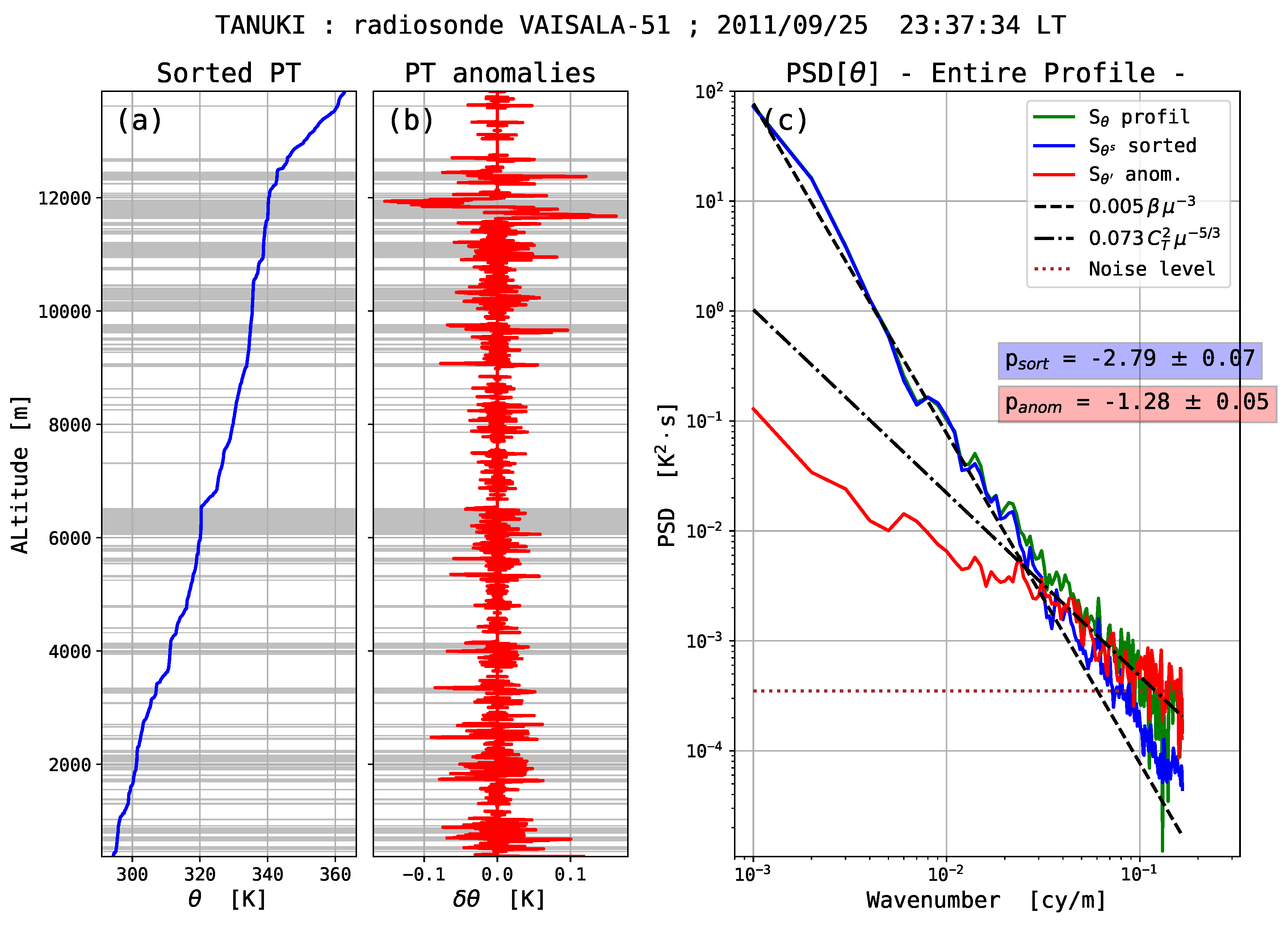
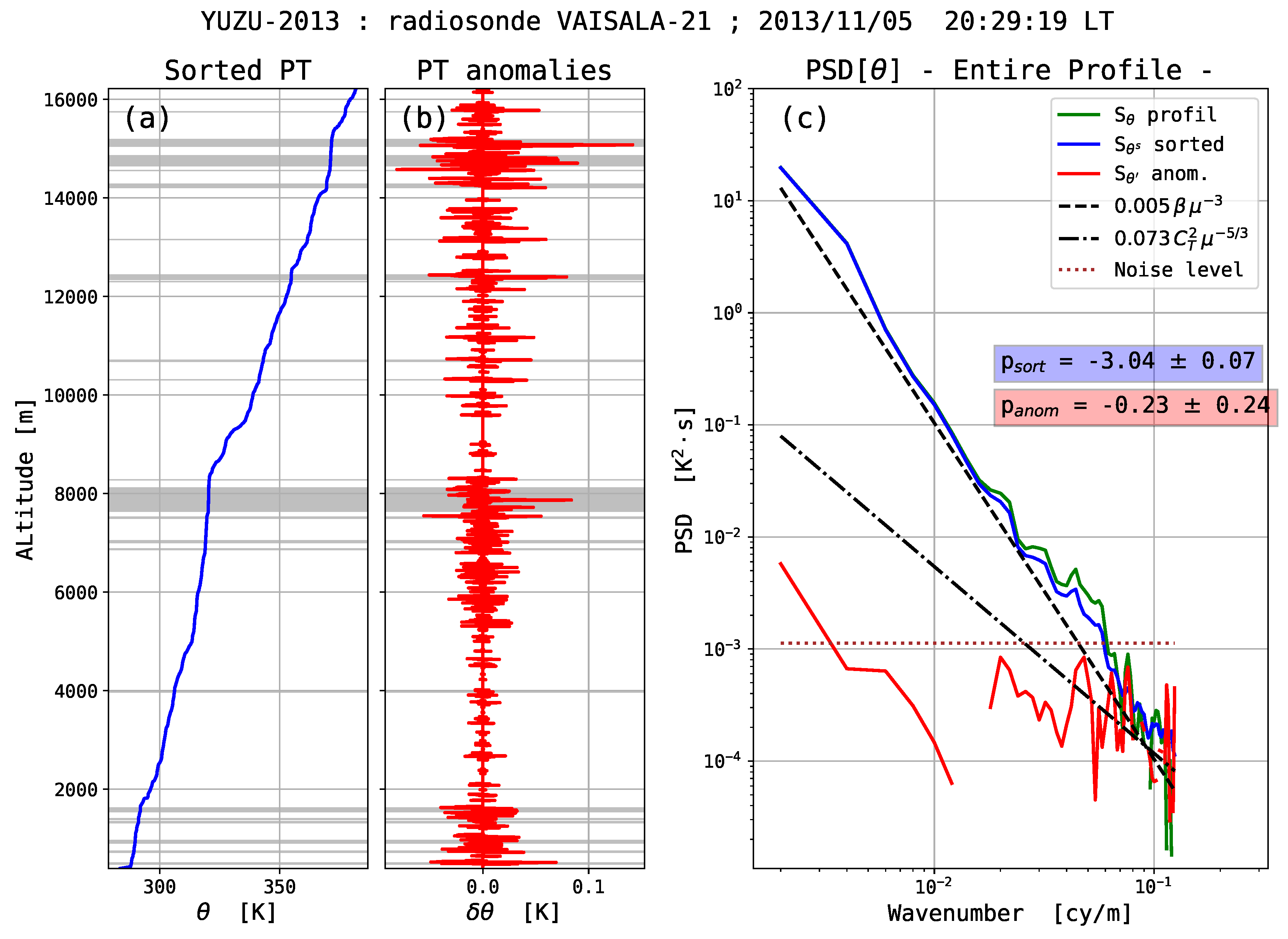
PT profiles for the entire troposphere have also been analyzed in terms of a sorted PT profile (stable everywhere) and an anomaly profile defined as the difference between the observed and sorted profiles. The sorted PT profile shows the state of minimum potential energy reachable by reordering adiabatically the observed profile [35]. It is the reference profile with respect to which the turbulent available potential energy (TAPE) created by the overturns (i.e., instabilities) in the flow is defined. This profile, which is stable everywhere (and will henceforth be referred to as an “everywhere-stable” PT profile), describes the state of vertical stratification of the atmosphere at a given moment. It is expected that the occurrence of turbulence leads locally in a reduction in static stability because of mixing. The spectral characteristics of the sorted PT profile therefore depend on the spatial distribution of layers with different static stability. These PSDs are found to be remarkably universal, varying as $m^{-3}$ for a domain of scales ranging from a few meters to a few hundreds meters. An interpretation of the sorted profile as a random superposition of layers more or less strongly stratified is proposed.

The anomaly profiles describe the PT differences between the sorted and observed profiles resulting from the vertical displacements of air parcels. Vertical displacements or PT differences are thus related to the TAPE consecutive to instabilities in the flow. The power spectra of these anomaly profiles provide information on the spectral characteristics of TAPE. To our knowledge, such a spectral analysis of reference (sorted) profiles and anomaly profiles has not been conducted yet.

The paper is structured as follows. Section 2 presents briefly the data set on which this study is based, as well as the data processing methods. The results are shown in Section 3. We also present an interpretation for the spectral characteristics of the sorted PT profiles. Section 4 contains a general discussion about these results aimed at describing some of the properties of the vertical stratification of the free atmosphere. Conclusions are drawn in Section 5.

2. Dataset and Data Processing Methods

2.1. The Dataset

Four measurement campaigns combining the Middle and Upper atmosphere (MU) radar and sounding balloons measurements took place at the Shigaraki observatory (34${}^{\circ }$51’ N, 136${}^{\circ }$06’ E), in Japan, from 2011 to 2014. These campaigns have been named TANUKI-2011, YUZU-2012, YUZU-2013 and YUZU-2014. They will be here noted for short as T11, Y12, Y13 and Y14. There were 111 meteorological balloon flights during these four campaigns. In the following of the paper, a particular flight will be designated by the campaign name and a flight number, for instance T11-34. A description of some of these MU radar-radiosondes campaigns, as well as results based on concurrent observations, are described elsewhere [15,16,36]. Further details about the four campaigns are listed in

Table 1. The 111 flights during four field campaigns held at Shigaraki (Japan). The rightmost column shows the number of balloon flights and, between parenthesis, the number of retained flights for the present study.

Campaigns		Date	# Flights (Selected)
TANUKI-2011	(T11)	2011/09/10-27	59 (33)
YUZU-2012	(Y12)	2012/11/03-07	6 (4)
YUZU-2013	(Y13)	2013/11/01-08	35 (16)
YUZU-2014	(Y14)	2014/10/02-10	11 (2)
total			111 (55)

.

The present work is exclusively based on the raw profiles of standard (operational) radiosondes. With a sampling rate of 1 Hz, the vertical resolution of the raw measurements is usually ∼5–6 m. For the purpose of turbulence detection, and following the suggestion of [37], most of the balloons were under-inflated, allowing a slower vertical motion and thus a better vertical resolution, typically ∼3 m.

Because the noise level on the temperature data is highly variable, mostly depending on the launching time (see Section 2.3), only night flights were selected, that is 55 flights (see Table 1).

2.2. Data Processing

The processing of the raw radiosondes profiles for the Thorpe analysis is now briefly summarized, the interested reader can find a more detailed description in [6,7,8]. The profiles of temperature, pressure, and humidity are resampled by linear interpolation with a regular vertical step. The vertical sampling resolution is the integer value (in meters) closest to the median of the measured (variable) vertical steps. Because the static stability in reduced in saturated air, i.e., in clouds, the Thorpe sorting is applied to a potential temperature ${\theta }_{*}$ which results from the numerical integration of the squared BV frequency $N^2$, which takes its “dry” expression for non-saturated air, and a “moist” expression for saturated air [38,39,40]. Instrumental noise can have a tremendous effect by generating artificial overturns. Wilson et al. [6], Wilson et al. [7] proposed an objective method to address the noise problem:

• The profile of the noise level of temperature measurements T is estimated from second order statistics on the nth order differences of short segments (∼60 m) of the T profile.
• An intermediate profile is built by subsampling and filtering the raw PT profile, ${\theta }_{*}$. A sorted profile ${\theta }_{*}^s$ is calculated. The algorithm is adaptative in the sense that the subsampling factor depends on both the noise level and on the background stability. It is chosen in order that the first differences in the sorted and subsampled profile ${\theta }_{*}^s$ are, in the average, significantly larger than the noise level, typically 3 times larger. The raw profile is subsampled by a factor of 3 to 7, the vertical resolution being reduced to ∼9–35 m. This intermediate profile is only used for the detection of the turbulent regions.
• The unstable regions are identified from the occurrence of inversions in the intermediate profile of ${\theta }_{*}$. In the present context, the word “inversion” does not have the sense used in meteorology describing an increase in temperature with altitude, but rather describes a decrease of potential temperature with altitude.
• A statistical test is performed on each detected inversions in the PT profile in order to recognize the ones which are very likely not due to noise.

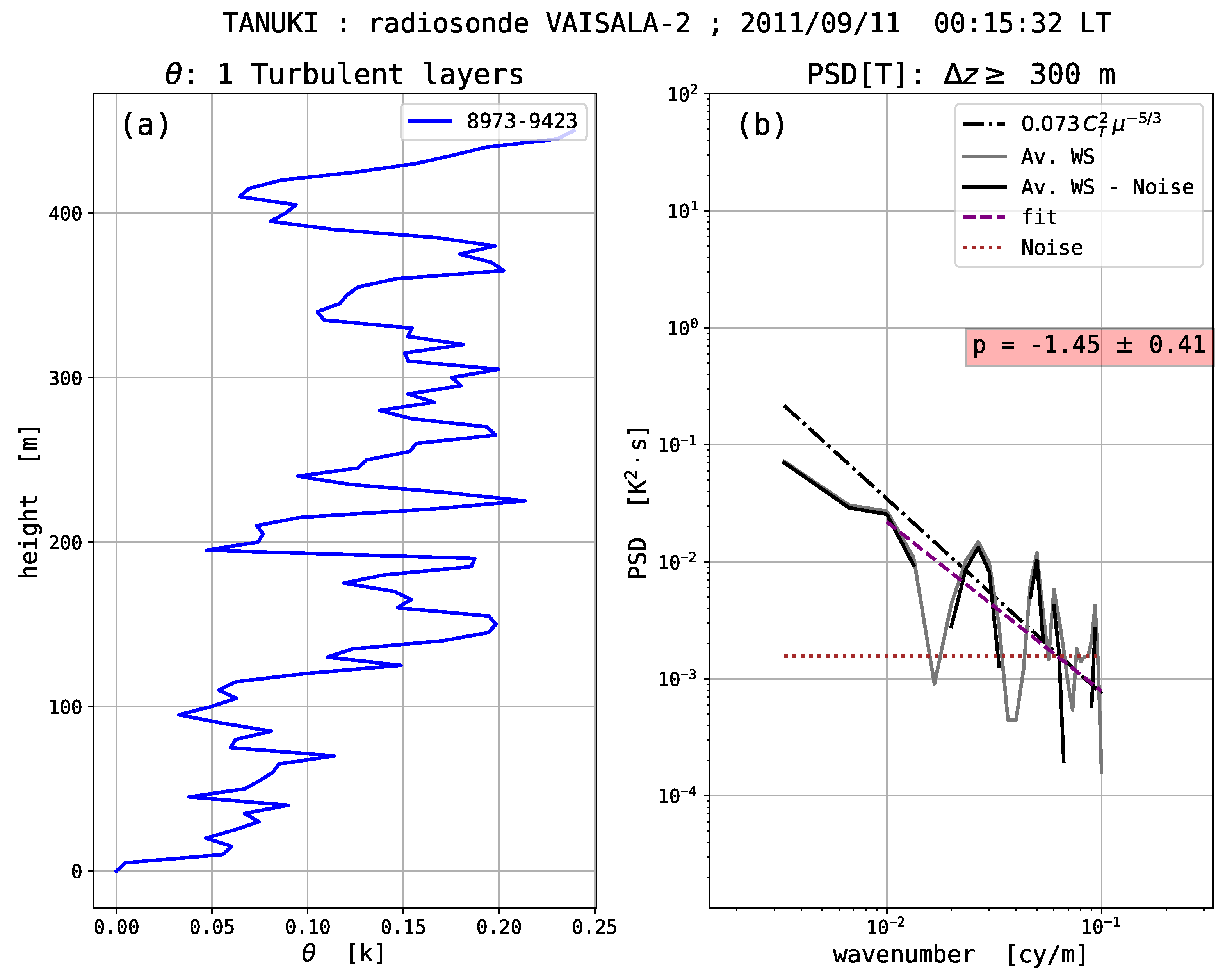
Figure 1 illustrates the principle of detection of unstable layers by the Thorpe method. It shows (a) the observed and sorted subsampled PT profiles, (b) the Thorpe signal defined as the difference between the observed and sorted profiles, ${\theta }_{*}-{\theta }_{*}^s$, and (c) the Thorpe displacements, that is the vertical distances air parcels have been displaced from the sorted profile to the observed profile.

At this point, it is important to stress that any unstable region is confined within a well defined layer, that is, a region for which the fluid parcels are adiabatically exchanged with others belonging to the same region. Formally, this property translates into the fact that the sum of the air parcels displacements is zero on a layer. Of course, the stable regions are also isolated since no air parcel for such a layer may come from any other layer.

2.3. Noise Level on T Profiles

A key point of this analysis relies on the estimation of the noise level on the measured temperature profiles. The noise level is quantified through the standard deviation of the T fluctuations presumably due to noise, i.e., of the uncorrelated fluctuations. For each sounding the noise profile of T is estimated empirically from the variance of the n order differences estimated on short data segments, 15 bins typically (45 to 75 m, depending on the vertical resolution).

The procedure of noise estimation is now described. The basic hypothesis is that a measurement sequence is composed of a correlated physical signal plus a random uncorrelated and centered noise. i.e., $X_i={\tilde{X}}_i+b_i$ where $X_i$ is the measured signal (bin i), ${\tilde{X}}_i$ is the physical (“true”) signal and $b_i$ the random noise. Let ${\sigma }_b^2$ be the variance of noise b.

The method consists of estimating the noise level, i.e., ${\sigma }_b$, from the variance of the nth order differences. The variance of the first order difference $\delta X_i=X_{i+1}-X_i$ is a good estimate of $2{\sigma }_b^2$ provided ${\tilde{X}}_{i+1}={\tilde{X}}_i$, that is if the “true” signal ${\tilde{X}}_i$ is constant whatever the value of i in the sequence. The expectation of the variance of the second order differences, ${\delta }^2{X}_i=\delta X_{i+1}-\delta X_i$ is $6{\sigma }_b^2$ provided ${\tilde{X}}_{i+1}={\tilde{X}}_i+a\Delta z$, i.e., $\tilde{X}$ increases linearly with z in the sequence. Calculating the variance of the nth order differences estimates ${\sum }_{k=0}^n{\left(C_n^k\right)}^2{\sigma }_b^2$, provided the ${\tilde{X}}_i$ profile is a polynomial of order $n-1$ of z.

Practically, the noise level is estimated on the entire temperature profile from the variance of the third or fourth order differences estimated on short overlapping and detrended data segments (15 bins typically). A noise profile is thus estimated from which a mean level of noise is computed. It is found that the estimate of noise level becomes weakly dependent of the order of differentiation n for $n\ge 3$.

From one flight to another, the mean temperature noise levels vary over more than one order of magnitude, from ∼5 mK to 100 mK. Figure 2 shows the mean noise levels according to the launching hour. It is obvious that daytime profiles are much noisier than night-time profiles since all daytime data have noise levels above 30 mK, while night-time data have noise levels below 30 mK. It is very likely that the excess noise during daytime is due to the effects of solar illumination on the temperature sensor coupled with its randomly varying orientation.

In fact, the most noisy profiles do not allow this study to be conducted because the power spectra at small-scale, i.e., for scales less than ∼50 m, are dominated by noise. It will be shown that this is not the case for the least noisy profiles since the (white) noise floor is only observed in the large wavenumbers of the spectra, i.e., for scales less than ∼10 m. Consequently, the day profiles were discarded. Of course, retaining only night flights limits the scope of this work as only conditions without deep convection will be considered.

2.4. Spectral Analysis

Unstable layers, presumably turbulent, thicker than 30–50 m can be detected from operational radiosondes [7]. The other regions do not show any PT inversions, or only a few inversions attributed to instrumental noise. These stably stratified regions will be called “calm” as opposed to turbulent ones. The power spectral density (PSD) of the temperature fluctuations are estimated for both the turbulent and calm regions.

In order to estimate the spectra over a sufficient range of scales, only layers thicker than a threshold $L_{\mathrm{seg}}=200$, 300 or 500 m were retained. Therefore, the domain of scales of interest ranges between a few meters (the Nyquist scale is ∼6–10 m) and ∼100–200 m typically (since the very first bins of the spectra are sensitive to the detrending method). For each identified layer, an average spectrum is estimated by averaging the spectra calculated on overlapping data segments of length $L_{\mathrm{seg}}$. For each segment, a linear trend found by joining the end points is removed [41] before multiplication by a Blackman window. Two spectral estimators were compared: the Welch spectrum [42], and the Maximum Entropy Method (MEM) spectrum [43]. No noticeable difference is observed between these two estimators, so only the Welch estimates are shown.

As a second step, the entire PT profile is analyzed as the sum of a sorted PT profile (stable every were) and an anomaly profile defined as the difference between the observed and sorted profiles. Power spectra are estimated for these two profiles in the domain of scales ∼10 to 1000 m.

As suggested by an anonymous reviewer, the time constant of the temperature sensor must be taken into account in the spectral analysis of the raw data. The time constant $\tau$ (63.2%) of the T sensor varies with pressure, P. According to the manufacturer (Vaisala, radiosondes RS92), $\tau \le 0.4$ for $P=1000$ hPa and $\tau \le 1$ s for $P=100$ hPa (i.e., $z\approx 17$ km). For a given pressure, the time constant $\tau \left(P\right)$ is estimated by a linear interpolation between these two values. By assuming a linear response of the T sensor, the transfer function reads $H\left(f\right)=1/(1+j2\pi f\tau )$ where f is frequency. The PSD estimate should thus be corrected as:

$$S_c\left(f\right)=S\left(f\right)\left(1+{\left(2\pi f\tau \right)}^2\right)$$

(6)

where S and $S_c$ are the computed and corrected PSD, respectively. This correction significantly affects the high frequency part of the power spectrum by “whitening” it (see figures below). As a consequence of the time-constant correction, the large wavenumbers part of the power spectra are now consistent with the noise level estimated from the nth order differences. By assuming that the noise is white, a spectral noise amplitude is estimated and subtracted from the PSDs. In most cases, this correction only affect the very large wavenumber part of the spectra, corresponding to vertical scales of ∼10 m or less (see Figures 6–9).

In order to perform the Thorpe analysis, the pressure and temperature profiles must be resampled regularly. Such a resampling procedure is a necessary step to construct two PT profiles, observed and sorted, with the same height steps. The resampled bins are here linearly interpolated from the original sampled measurements. They are thus weighted averages of two consecutive measurements of the original profile, the weightings being random. Consequently, the PSDs must be considered with some caution for wavenumbers close to the Nyquist wavenumber, due to the low-pass filtering induced by this resampling procedure.

The spectra are here presented according to “spatial frequency”, i.e., to vertical wavenumbers expressed in (cy/m). Such a graphic presentation is much easier to read. On the other hand, it leads to expressions of well-known relationships with somewhat unusual constants. Thus, the OC turbulent spectrum (Equation (1)) expressed as a function of “spatial frequency” $\mu =m/2\pi$ reads:

$${S^{\prime }}_T^{\mathrm{turbu}}\left(\mu \right)=2\pi S_T^{\mathrm{turbu}}={\displaystyle \frac{0.25}{{\left(2\pi \right)}^{2/3}}}{C}_T^2{\mu }^{-5/3}=0.073C_T^2{\mu }^{-5/3}$$

(7)

since $S_T\left(m\right)dm=S_T^{\prime }\left(\mu \right)d\mu$. Expressed as a function of the “spatial frequency” $\mu$, the temperature PSD of saturated gravity waves (Equation (2)) reads:

$${S^{\prime }}_T^{\mathrm{IGW}}\left(\mu \right)=2\pi S_T^{\mathrm{IGW}}={\displaystyle \frac{A}{4{\pi }^2}}{\displaystyle \frac{N^4{\overline{T}}^2}{g^2}}{\mu }^{-3}$$

(8)

By defining $\beta =N^4{\overline{T}}^2/g^2$, and by taking $A=0.2$, the IGW spectral model can be written:

$${S^{\prime }}_T^{\mathrm{IGW}}\left(\mu \right)={\displaystyle \frac{A}{4{\pi }^2}}\beta {\mu }^{-3}=0.005\beta {\mu }^{-3}$$

(9)

The PSD estimates for the stable and unstable layers, and for the entire PT profiles, will be compared to these two models (Equations (7) and (9)).

3. Results

First, two statistics of the detected stable and unstable layers are described: thicknesses and Brunt-Väisälä frequencies. The Brunt-Väisälä (BV) frequency quantifies the static stability within the layers (Equation (3)). Then the spectral characteristics within calm and turbulent layers thicker than thresholds of 200, 300 or 500 m are shown. Finally, power spectra of the entire PT profiles are presented.

3.1. Thickness Distribution of the Detected Layers

Figure 3 shows the histograms of the layers thicknesses detected by the Thorpe method for all the flights of the four campaigns (111 flights). The upper (lower) panel shows the thickness distribution for the turbulent (calm) layers, respectively. The black stair-like histograms show the distributions of the layers thicker than 200 m obtained from the least noisy soundings, i.e., the layers from which spectral characteristics are evaluated (see next section).

The limits of the classes of the two histograms shown in Figure 3 are powers of 2, i.e., 8–16 (m), 16–32, etc. Very likely, the numbers of occurrences for the two first classes are subject to side effects since the vertical resolution of the intermediate profiles (used for turbulence detection) depends on the noise level of the soundings. The higher the noise level, the coarser is the vertical resolution. The number of detected unstable layers thinner than 32 m is likely very dependent on the vertical resolution. However, for thicknesses larger than 32 m, that is from the third class, such a side effect should be negligible. The number turbulent layers is found to be a decreasing function of thickness (for layers thicker than 32 m).

With regard to the stably-stratified layers (Figure 3b), it should be noted that their thicknesses are nothing other that the intervals between the detected unstable layers. Consequently, their distribution of thicknesses should not be sensitive to side effects in the way the detected layers are. However, this distribution likely depends on the vertical resolution of the soundings, but in a way it is difficult to assess. Thus, the distribution of the stable layers thicknesses can be affected by the low detectability of the thin unstable layers. For the present resolution, the thickness distribution shows a mode at ∼100–200 m.

Figure 4 shows the histogram of the layers thickness (same as Figure 3a) but on a log–log plot. The empirical distribution is found to follow a power law approximately, the empirical PDF of the unstable layers thicknesses h varying as $h^{-r}$, with $r=2.1\pm 0.1$, at least for layers thicker than ∼30 m. Wilson et al. [7] (their Figure 7) showed a distribution of the turbulent layers thicknesses detected by the Thorpe method applied to very high-resolution soundings ($\delta z\sim 10$ cm). This distribution approximately follows a $-1$ power law. From a large dataset of 3523 soundings over the Indian Ocean, Bellenger et al. [12] also observed a decreasing distribution of the overturns sizes. However, their results suggest (i) an exponential law for the empirical PDF of thicknesses (as the log of the distribution decreases almost linearly with the sizes) and (ii) that there is no universal behavior in that matter since they observed different distributions for different regions of the troposphere.

3.2. Distribution of the Squared Brunt-Väisälä Frequencies

The vertical static stability of the layers is quantified through the squared BV frequency, $N^2$ (Equation (3)). BV frequencies are estimated from the sorted PT profiles for both the unstable and stable layers. For every layer, unstable or stable, the vertical component of the $\theta$ gradient is estimated as the range of PT on that layer divided by its thickness, the average $\overline{\theta }$ being calculated on the layer. Figure 5 shows the normalized distributions of BV frequencies, i.e., the empirical probability density functions (PDF), estimated (a) for the unstable layers and (b) for the stable ones. The black stair-like histograms correspond to the selected layers for the spectral analysis, i.e., thicker than 200 m from the least noisy profiles. The mean values of $N^2$ associated with these distributions are indicated in the colored boxes (the means corresponding to the thicker layers are indicated within the parentheses).

The two empirical distributions are observed to be significantly different since the mean $N^2$ of the stable layers is about 2.5 times larger than that of the unstable layers. The contrast is even higher (a factor of 5) for the selected layers (thicker than 200 m from the low noise level profiles). Also, the two histograms have different symmetries, the one corresponding to the unstable layers having a positive skewness (left modal), the other one a negative skewness. These findings show that the static stability is smaller within the unstable layers selected by the Thorpe method, the BV frequencies being smaller by a factor 2.5 to 5. These results are very similar to those of Bellenger et al. [12] and Alisse and Sidi [2]. Such a reduction in static stability within the unstable layers is very likely the consequence of turbulent mixing.

3.3. The Spectral Characteristics of the Unstable and Stable Regions

Vertical PSDs are estimated for both calm and turbulent regions from layers thicker than 200, 300 or 500 m, depending on the distribution of the layers thicknesses of the flights. As a first step, a few examples of the spectral features of layers, unstable or stable, of some flights are presented (e.g., Figure 6). Then, averaged power spectra of the unstable and stable layers determined from several flights are shown (e.g., Figure 7, Figure 8 and Figure 9).

3.3.1. Some Examples of Spectra of Unstable and Stable Layers

Figure 6 shows one example of a single unstable layers for flight T11-2. The left panel shows the vertical PT profile shifted in order to be zero at the bottom of the layer, i.e., ${\theta }_{\mathtt{shift}}\left(z\right)=\theta \left(z\right)-\theta \left(z_{\mathrm{bottom}}\right)$. The vertical axis corresponds to the height of the layer relatively to the bottom height. The altitude range of the layer in indicated as the legend of the curve. The right panel shows the corresponding power spectrum. The atmospheric conditions during this particular flight were very quiet since only one unstable layer deeper than 300 m was detected (the only one detected is 450 m thick). The horizontal dotted line shows the noise level by assuming a white noise, the noise variance being estimated by the method presented in Section 2.3. The gray and black curves correspond respectively to the calculated spectrum (taking into account the time constant correction described in Equation (6)) and to the “corrected” spectrum obtained by subtracting the white noise level. The dashed straight line shows the linear regression of the corrected spectrum in log-log coordinates, in the wavenumber range 10${}^{-2}$–10${}^{-1}$ m${}^{-1}$. The slope of the linear fit as well as its standard deviation are indicated in the colored box. The dot-dashed line shows the OC spectrum (Equation (7)), the structure constant $C_T^2$ being inferred from the linear fitting. The spectral index is found here to be $p=-1.45$. However, the single-layer PSD estimate appears very noisy for estimating a slope with an acceptable confidence since the standard deviation of the slope is as large as 0.41. It is necessary to average several spectra in order to reduce the noise of the PSD estimates.

An example of an averaged power spectrum is shown in Figure 7. Five unstable layers thicker than 300 m are detected during flight T11-49 (Figure 7a). The thicknesses of these layers range from 333 to 504 m. The right panel shows the mean power spectrum estimated as the weighted geometric average of the five spectra, the weightings being proportional to the thickness of each individual layer, or more precisely to the number of spectra contributing to the Welch spectrum of that layer. The corrected spectrum obtained after subtraction of the noise level is shown as a thick black curve. The spectral index estimated from a linear fit in the wavenumber domain 10${}^{-2}$–10${}^{-1}$ m${}^{-1}$ is $p=-1.57\pm 0.13$. The averaged spectrum for the unstable layers is observed to to be consistent, within a factor of two, with a $-5/3$ power law for the corresponding domain of scales.

Figure 8 shows the features of 9 stably-stratified (i.e., calm) layers for the same flight T11-49. The thicknesses of these layers range from 414 m to 1467 m for heights between 2994 and 15432 m. The corresponding mean PSD is shown in Figure 8b. The contrast with the mean PSD of the five unstable layers of this flight (Figure 7b) is evident. The mean spectrum follows a steep power law, $p=2.56\pm 0.09$, for scales ranging from ∼10 to 100 m. The dot-dashed line shows the theoretical power law for a saturated gravity wave spectrum (Equation (8)) by estimating the $\beta$ factor ($\beta =N^4{\overline{T}}^2/g^2$) as the weighted average on the 9 considered stable layers. The experimental PSD is consistent within a factor of two with the IGW model.

Figure 9 shows another example of stably-stratified regions, this time from flight Y13-21. Eleven stable layers thicker than 300 m are observed, thicknesses ranging from 398 m to 2042 m, for altitudes between 1893 and 16,209 m. Figure 9a,b shows the vertical (shifted) PT profiles and the corresponding averaged power spectrum, respectively, with the black curve showing the corrected mean PSD. This mean PSD is well described by a power law with a slope $p=-2.76\pm 0.14$, down to a vertical scale of ∼10 m. A remarkable finding is that not any transition toward an inertial domain, i.e., with a $-5/3$ power law, can be observed for vertical scales smaller than ∼30–50 m, that is for scales smaller than that of the detected inversions. The ∼−2.8 spectral domain appears to extend down to scales of a few meters. This last result suggests an important conclusion: there does not seem to be any background turbulence, and therefore no instability, at scales below the detection threshold ∼30 m, at least for the stable layers of this flight. In other words, the flow appears to be laminar down to vertical scales of ∼10 m within these stable layers. This conclusion appears to be valid for most of the stable layers (from the low noise profiles).

3.3.2. Spectral Characteristics of the Unstable and Stable Layers From the Averages on Several Flights

Figure 10 shows the mean spectra for both the unstable and stable layers from 16 flights, T11-44–59, during the September 2011 campaign. 41 unstable layers and 109 stable layers thicker than 300 m are detected. The linear fits (dashed straight lines) are estimated in the 10–100 m domain of scales. The turbulent (OC) and saturated IGW models are shown (dot-dashed lines) with $C_T^2$ and $\beta$ estimated by averaging on the retained layers. The averaged white noise levels is also shown (dotted line). The spectral indexes for both averaged spectra are indicated in the colored boxes.

A very clear difference in the vertical power spectra according to the flow regime is observed. For the unstable regions, the mean spectral index is $-1.7\pm 0.07$, in very good agreement with the OC model of turbulence. For the stable regions, the vertical power spectrum varies as $\sim {\mu }^{-2.59}\pm 0.04$. The PSD amplitude of the stable layers is in fairly good agreement, within a factor ∼2.5 for scales of ∼100 m, with the theoretical spectrum of a saturated gravity wave field, that is $0.005\beta {\mu }^{-3}$. The two power spectra cross for $\mu \approx 4\times {10}^{-2}$ m${}^{-1}$, i.e., in the average, the T variance is larger in the unstable layers than in the stable ones for scales less than ∼25 m.

Another example of mean power spectra according to the flow regime is shown in Figure 11. The averaged spectra from 21 unstable layers and 151 stable layers, thicker than 200 m, for 13 flights of the Y12 and Y13 campaigns (November 2012 and 2013) are plotted. Again, the spectral indexes are significantly different depending on the state of stability of the layers: the spectral indexes is $-1.71\pm 0.09$ for the unstable layers, and $-3.04\pm 0.09$ for the stable ones, the linear fit being performed in the 10–100 m scales domain. The power spectra cross for a vertical scale of about 40 m.

3.3.3. Statistics of the Spectral Indexes of the Unstable and Stable Layers From All the Selected Radiosoundings

Table 2. Statistics on the spectral indexes p from 55 radiosonde profiles. The spectral indexes are estimated for the domain of scales 10–100 m. The mean p plus or minus the mean of standard deviations are indicated, as well as the average of the 95% confidence intervals.

Scale Domain (m)		p [Stable]	p [Unstable]
10–100	slope ± std. dev. 95% conf. interv.	$-2.79\pm 0.18$ $[-3.14,-2.44]$	$-1.72\pm 0.27$ $[-2.25,-1.19]$

shows the weighted averages of the spectral indexes p of the stable and unstable layers thicker than 300 m from all the selected flights. The averages of the standard deviations on the p estimates are also provided, as well as the averages of the 95% confidence intervals. Spectral indexes are estimated from a linear fit in the wavenumber intervals $[{10}^{-2},{10}^{-1}]$ m${}^{-1}$, i.e., for the scale domain 10–100 m. The spectral indexes of the unstable layers ($-1.72\pm 0.27$) are significantly different from the spectral indexes of the stable layers ($-2.79\pm 0.18$).

This last finding strongly suggest that developed turbulence is observed in most of the unstable layers, since mean power spectra are consistent with the OC model of inertial turbulence. In contrast, the spectra of the stable layers are roughly consistent with the models of saturated IGW or BSR, although the mean spectral index (−2.8) is slightly higher than −3. For most stable layers, no transition to turbulence is observed for scales less than the detection limit of the Thorpe method (30–50 m). This last observation suggests that, in most cases, the flow is laminar down to vertical scales of ∼10 m the within the stable regions. Finally, the fact that the spectral indexes have clear distinct values according to the detected static stability, and that these values are consistent with theoretical models for turbulence and IGW (or BSR), support the conclusion that the careful application of Thorpe’s method on standard radiosondes, at least on those least noisy profiles, allows discrimination between turbulent and laminar flow regimes in the atmospheric column.

3.4. Spectral Analysis of the Entire PT Profiles

In principle, Thorpe’s method consists in comparing a potential temperature profile to the same profile sorted. The difference between the observed profile $\theta$ and the sorted one ${\theta }^s$ defines an anomaly profile ${\theta }^{\prime }$ as

$${\theta }^{\prime }\left(z\right)=\theta \left(z\right)-{\theta }^s\left(z\right)$$

(10)

where z is altitude. Since several regions in the profile are unstable, likely turbulent, we expect the anomaly profile to be constituted with a succession of layers, some showing turbulent PT fluctuations, and others with almost no fluctuations, indicating stability everywhere. The spatial distribution of the “shaky” layers is a signature of the spatial distribution of the unstable layers, that is of the spatial intermittency of turbulence. Another signature of turbulence intermittency can be seen in the sorted PT profile as it is expected to be comprised of a succession of strata more or less stably stratified, with the weakly stratified regions showing local mixing of the turbulent layers. The question now addressed is about the power spectral density of these two profiles for small to meso scales, that is for vertical scales ranging from ∼10 m to 500 m.

Figure 12a,b shows the sorted and fluctuations profiles for flight T11-51. The shaded areas show the positions and depths of the detected unstable, i.e., turbulent layers. For this particular flight, 43% of the anomaly profile is zero, that is no overturn is detected for that fraction of the profile.

The PSD estimates for the observed PT, sorted PT and anomaly profiles are shown in Figure 12c. The averaged Welch spectra are here calculated on data segments 1000 m long. The noise variance is estimated on the entire PT profile. The horizontal dotted line shows the corresponding spectral level of noise by assuming it is white. The PSDs of the observed and anomaly PT profiles are corrected for both the time constant (Equation (6)) and for the noise level. However, since a majority of data bins are displaced in the sorted PT profile, the effect of the time constant of the T sensor are presumably “randomized” in the vertical. Consequently, the PSD of the sorted PT profile cannot be corrected according to Equation (6). Also, a noise floor is not observed on the sorted PT spectra. (Indeed, if one assumes a profile containing only uncorrelated noise, the PSD of the sorted profile will follow a power law ${\mu }^{-2}$.) Because no clear spectral signature is evident, even in the large wavenumber part of the spectra, the power spectra of the sorted PT profiles are presented without noise correction. The power spectrum of the anomaly profile is approximately proportional to ${\mu }^{-1.3}$ over about 1 decade, up to vertical scales of ∼50 m. For larger scales, the spectral index is larger, close to ∼−1. The interpretation of this anomaly spectrum is not straightforward since 3 turbulent layers larger than 300 m, and 5 larger than 200 m, are detected for this flight. On the other hand, the spectrum of the sorted PTs (blue continuous curve) scales as $\sim {\mu }^{-3}$ over almost two decades, for vertical scales ranging from ∼8 m to 500 m. The amplitude of the sorted PTs PSD is consistent with the IGW model. The green curve shows the power spectrum of the observed PT profile. It is dominated by the power spectrum of the sorted PTs ($\propto {\mu }^{-3}$) for scales larger than 50 m, and by the anomaly spectrum ($\propto {\mu }^{1.3}$) for scales smaller than 50 m. (Strictly speaking, the PSD of the observed profile is not the sum of the PSDs of the sorted and anomaly profiles since if the Fourier Transform is linear, the power spectrum is not.)

Another example, flight Y13-21, is shown in Figure 13. The atmosphere is particularly calm for this flight since 62% of the anomaly profile is zero, i.e., no inversion detected. The green curve of Figure 13c shows the corrected PSD of the observed PT profile, the blue and red curves showing the PSDs of the sorted and anomaly PTs respectively. These spectra are here estimated on segments 500 m long. The spectrum of the sorted PTs is proportional to $\sim {\mu }^{-3}$ over more than one decade, down to a vertical scale of ∼10 m, and its amplitude is consistent with the IGW model. The PSD of the anomaly profile is below the noise level (after correction) for scales ranging from ∼10 to 250 m. This suggests that the $\theta$ anomalies are here mostly due to the random noise.

From the 55 selected flights, the mean spectral index of the sorted PT profiles is $p=-2.86\pm 0.09$ for the domain of scale 30–300 m, the mean 95% confidence interval is $[-3.04,-2.68]$. For the domain of scale 10–100 m, the mean spectral index is $p=-2.93\pm 0.09$, i.e., the 95% confidence interval is $[-3.11,-2.75]$.

The power spectra of the sorted PT profiles vary approximately as $\beta {\mu }^{-3}\equiv {\overline{\theta }}_z^2{\mu }^{-3}$ (${\overline{\theta }}_z\equiv \partial \overline{\theta }/\partial z$) down to scales of a few meters. This observation seems to be applicable to all the sorted PT profiles. What could be the reason? By noting that the anomaly PT profiles reveal the spatial distribution of the displaced data bins in the reordered profile, we see that the fraction of the displaced bins in the reordered profiles is frequently larger than 50% (38% for a particularly “quiet” atmosphere as shown in Figure 13a). Consequently, PT reordering affects a large fraction of the sorted profiles, due to both turbulent mixing and random noise. These displacements are however limited in the vertical, i.e., within layers of finite thicknesses. Now, we observe that the empirical PDF of thicknesses is a decreasing function of thickness. Consequently, the reordering procedure is thought to mostly affect the large wavenumbers part of the power spectra. Therefore, the power spectra of the sorted PTs can hardly be interpreted as saturated IGW or BSR spectra, especially for large wavenumbers.

It is assumed that the ∼${\mu }^{-3}$ power spectra of the sorted PTs reflect some properties of the vertical background stratification, showing an alternation of weakly and strongly stratified layers. Simple stochastic models aiming at simulating the vertical strata of the atmosphere can reproduce most of the spectral features of these everywhere-stable PT profiles.

3.5. A sTochastic Model for Describing the Stable Profile Corresponding to the State of Minimum Potential Energy

It is hypothesized that the sorted PT profiles carry the footprint of the turbulence intermittency through the spatial distribution of well-mixed regions within a globally stably stratified atmosphere. This assumption is based on the following observations:

• The regions where inversions (i.e., instabilities) occur are found to have smaller static stability, presumably because of turbulent mixing.
• The fraction of the PT profile for which the vertical stability is reduced due to diabatic mixing, i.e., the turbulent fraction, is frequently larger than 50%. That fraction of the sorted profile is altered by the sorting procedure.
• The distribution in thickness of these unstable layers varies approximately as $h^{-2}$ where h is the layer depth. The reordering procedure is thought to mostly affect the small scales of the sorted PT profiles.

It has been shown that the main features of the sorted PTs power spectra may result from the random spatial distribution of strata which are more or less stable. The vertical distribution of the mixed layers likely reflect the distribution of the instabilities in the atmospheric column. This hypothesis is tested through simple stochastic models based on the assumption that the PT increments have properties of a flicker noise. These models are presented in Appendix A.

4. Discussion

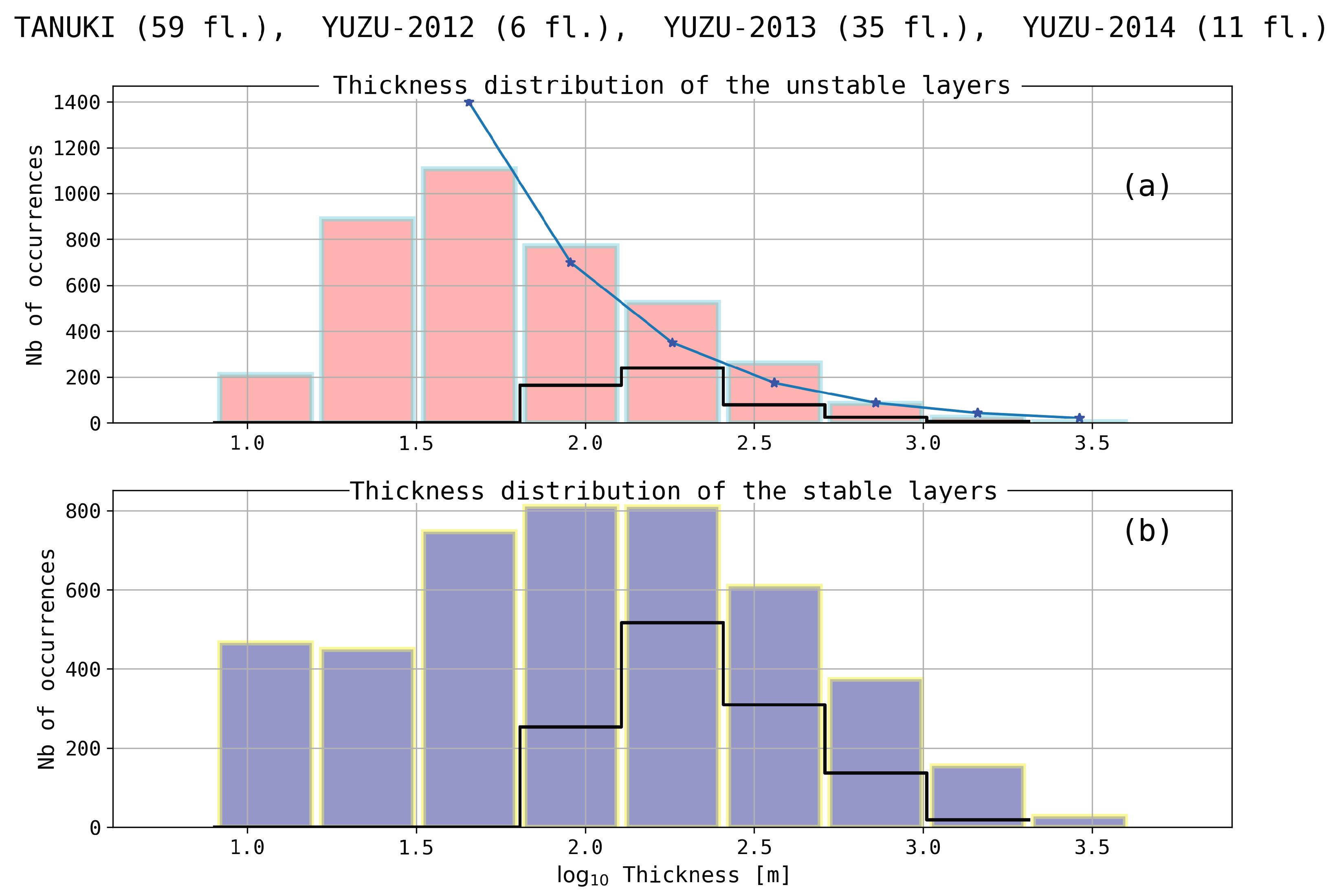
The first objective of this work has been to describe some statistical properties of the atmospheric layers identified by the Thorpe method from standard radiosondes observations. One important limitation of this study is that the usable observations are limited to night flights because of the relatively large instrumental noise of the day soundings. From these low noise soundings, the minimum size of the detectable unstable layers from the raw data of operational radiosondes is 30–50 m.

The histogram of thicknesses h of the unstable layers suggests a power law distribution varying as $h^{-r}$, with r close to 2, at least for $h>30$ m. However, this results does not seem to be universal, i.e., reproducible regardless of conditions, location, etc. The observations of [7] (their Figure 7), from very high resolution T soundings ($\delta z\approx 10$ cm), suggest a ∼−1 power law distribution of the unstable layers thicknesses. On an other hand, the findings of Bellenger et al. [12] from a large radiosoundings data base over ocean suggest an exponential distribution of these unstable layers thicknesses. These authors also observed different shapes of the thicknesses distributions for different regions of the troposphere.

The background static stability within the layers identified by the Thorpe method, whether stable or unstable, is quantified by the BV frequency estimated on the sorted PT profiles. It is found to be reduced by a factor 2.5 to 5 in the unstable layers comparatively to the stable ones. This last result is similar to those of [2,12]. Such a reduction in stability within the unstable layers is very likely the consequence of turbulent mixing.

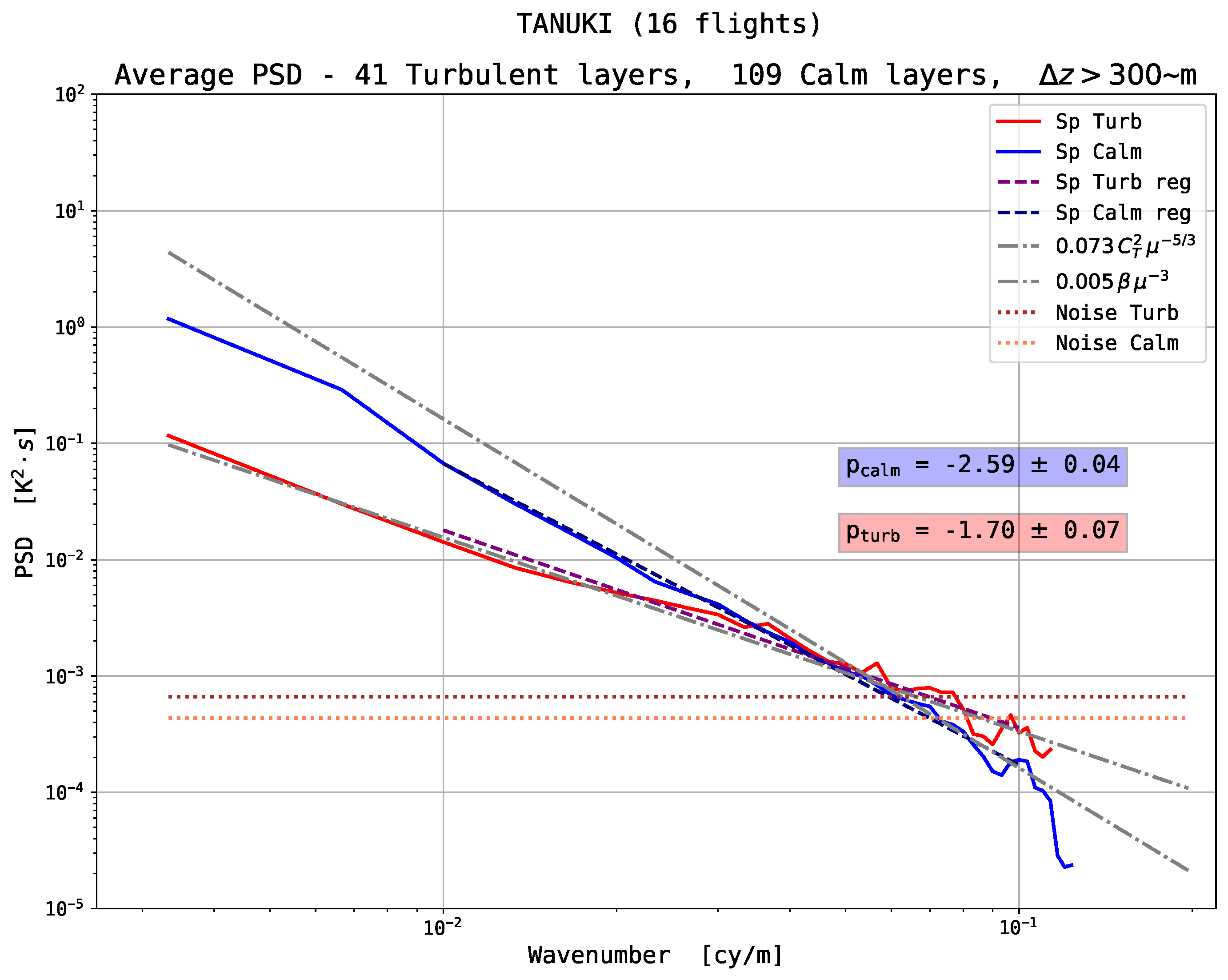
Power spectra of temperature fluctuations within the detected unstable and stable layers are estimated from the least noisy T profiles, that is profiles for which the standard deviation of noise is less than 12 mK. Power spectra are corrected for the time constant of the T sensor, a white noise level being then subtracted. It is shown that, on average, power spectra follow power laws with distinct exponents according to the static stability conditions. For vertical scales ranging from ∼10 m to 100 m, the spectral indexes are in the average $-1.7\pm 0.3$ for the unstable layers and are $-2.8\pm 0.2$ for the stable ones. These results validate the Thorpe method since the identified layers have clear distinct spectral characteristics. The averaged T PSDs of the unstable layers are consistent with the Obukhov-Corrsin model of temperature turbulence in the inertial domain. This suggests that turbulence is developed within most of the detected unstable layers. An obvious consequence is that it is possible to directly estimate the intensity of temperature turbulence, i.e., $C_T^2$, from the T profiles of standard radiosondes, at least from the least noisy ones. The averaged T PSDs in the stable layers, proportional to ${\overline{{\theta }_z}}^2{\mu }^{-3}$, compare well with the findings of [32]. These authors described the spectral characteristics of the T fluctuations for scales larger than 300 m in the troposphere and lower stratosphere. They observed the slope of mean T PSDs to be very close to $-3$ in the troposphere whatever the season, and a spectral amplitude close, within a factor of 3, to the one predicted by the IGW saturation theory (Equation (9)). The domain of scales considered in the present study is about on order of magnitude smaller than in the paper of Tsuda et al. [32]. However, the T PSD appear to be consistent with the saturated IGW, or BSR, spectral model down to vertical scales of ∼10 m. The only vertical spectra of the temperature fluctuations do not allow distinction between these two interpretations.

Such a spectral analysis of atmospheric layers according to their stability conditions suggests that the atmosphere is constituted of strata with distinct flow regimes. A remarkable finding is that no background turbulence is observed: in most of the stable layers for scales below the detection limit (∼30–50 m for the least noisy profiles), since no change in the spectral slope is visible (on the averaged PSDs). These stable layers show characteristics of a laminar flow, that is no instability, and steep power law spectra (∼${\mu }^{-3}$), down to vertical scales of ∼10 m.

The spectral characteristics of the entire tropospheric PT profile, that is without distinguishing layers, are analyzed as the sum of a sorted profile and an anomaly profile, the anomaly profile being the difference between the observed and sorted PTs profiles. These anomaly profiles illustrate the turbulence intermittency of the atmosphere as they show a succession of puffs of variability, i.e., of PT fluctuations relatively to the sorted profile, separated by regions containing no fluctuation at all. The fraction of these everywhere-stable (non-turbulent) regions is commonly less than 40%. It can be in some cases larger than 60% (remember that only night profiles are considered here).

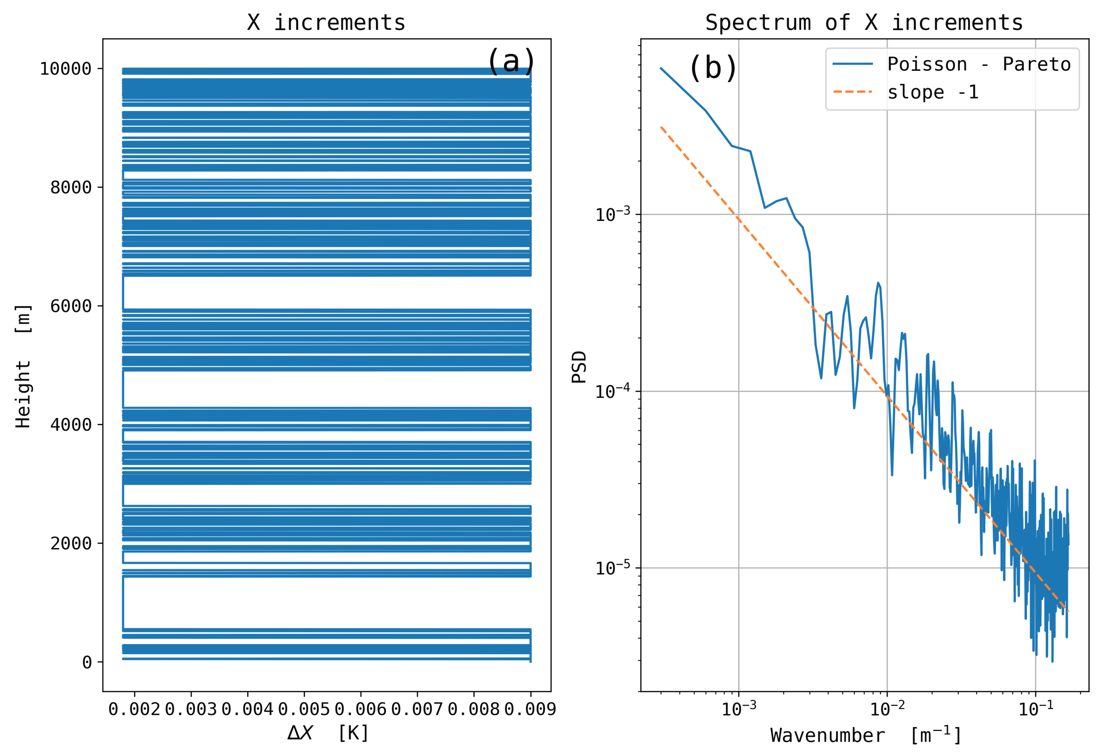
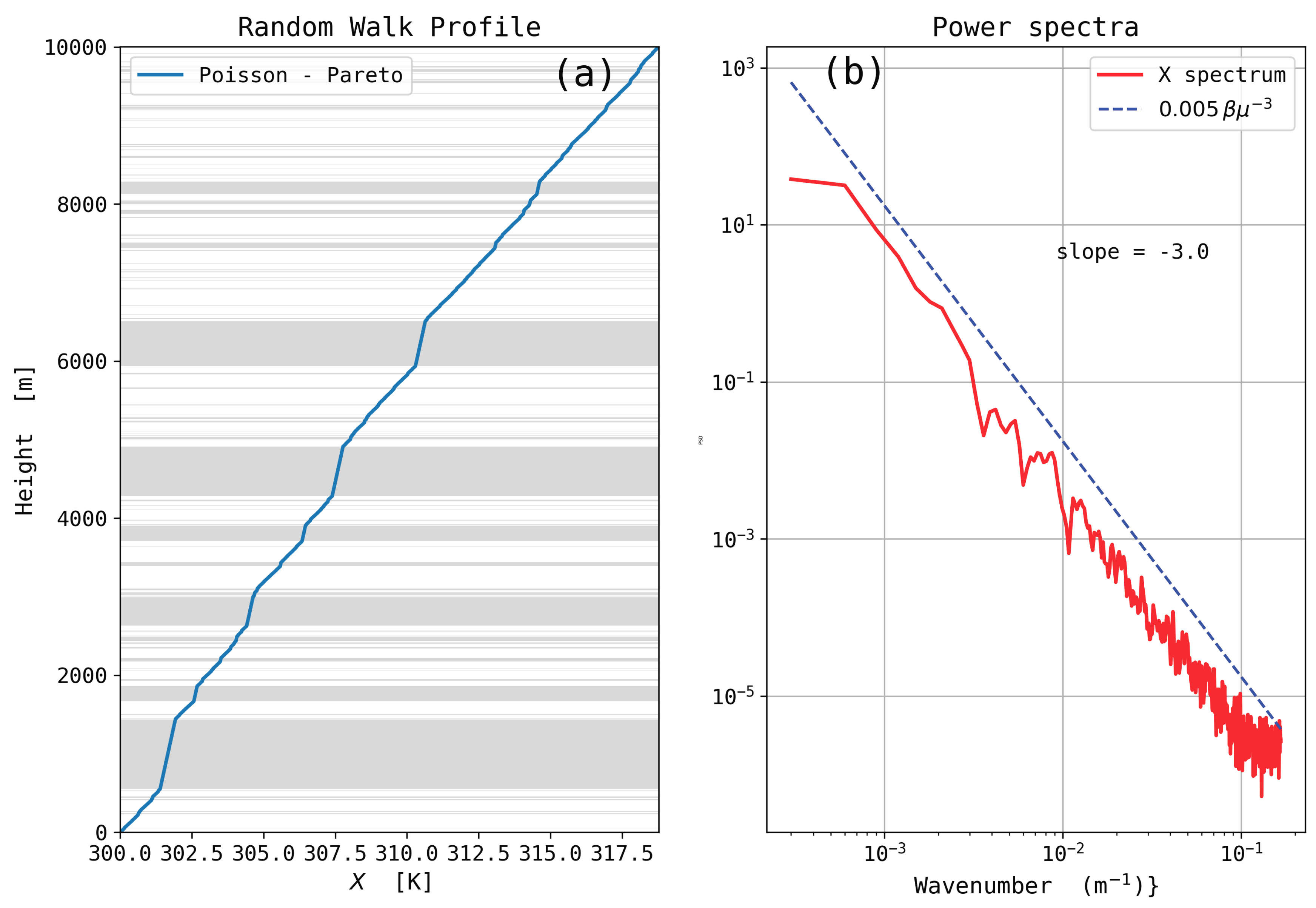
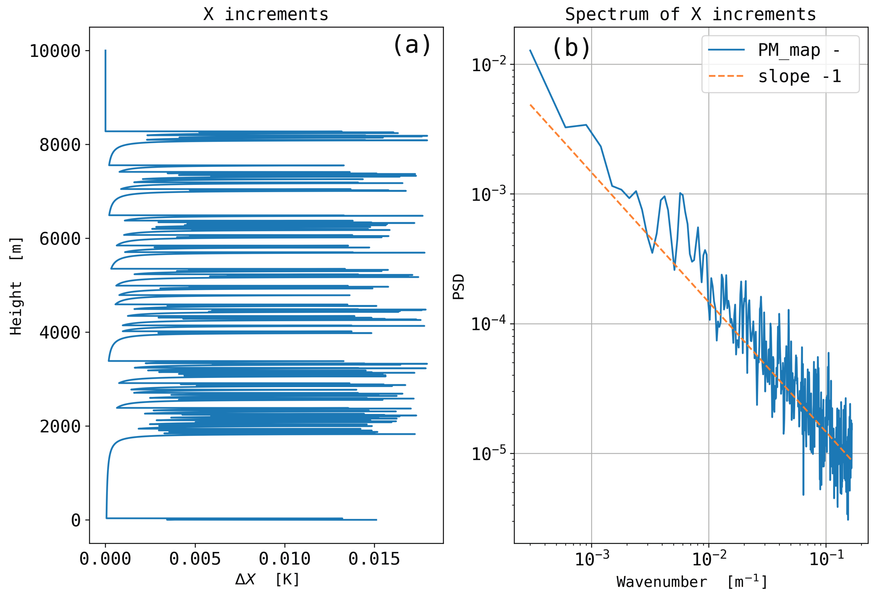
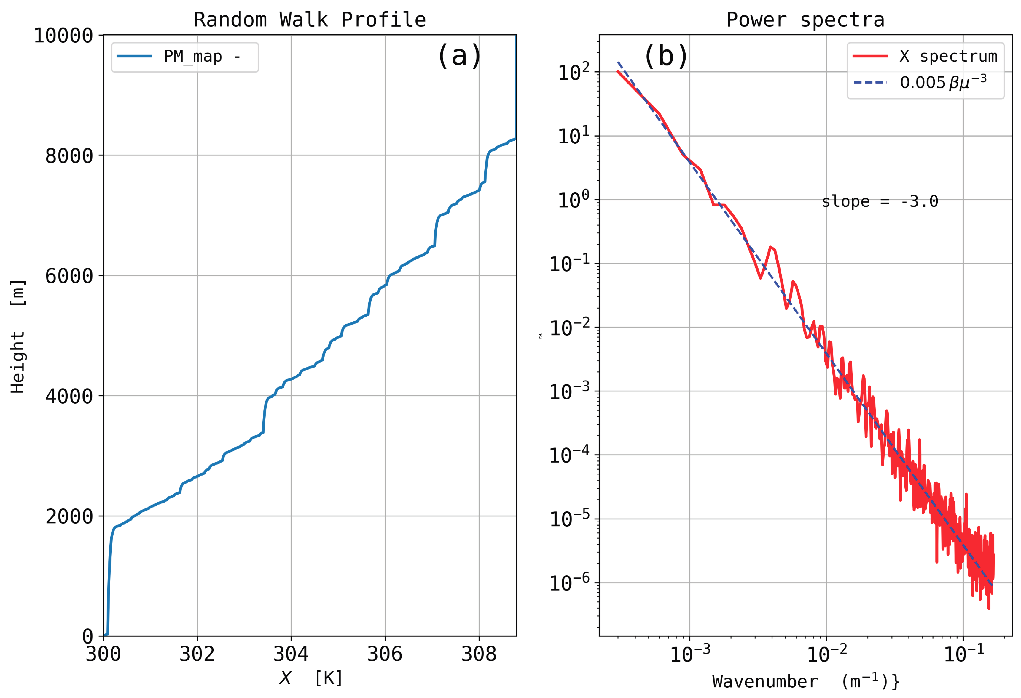
Interestingly, the PSDs of the sorted PT profiles are observed to be reproducible, scaled as ${\overline{\theta }}_z^2{m}^{-3}$ down to scale of a few meters. These everywhere-stable PT profiles results from an adiabatic reordering of the observed (measured) PT profiles. They describe the state of potential energy minimum achievable from the observations. It is assumed that the spatial distribution of the weakly stratified regions is random, resulting from the turbulence intermittency. Sorted PT profiles are simulated based on random walks with positive increments having properties of a flicker (1/f) noise. Intermittent processes are known to produce such $1/f$ spectra [44,45,46], that is a spectral index between 0 (the white noise) and $-2$ (the Brownian noise). Positive increments here reflect the vertical stratification of the atmosphere, i.e., $\delta \theta =(\partial \theta /\partial z)\delta z$. It is thus assumed that the PSD of the positive increments of $\theta$ follows a ${\mu }^{-1}$ power law as a consequence of turbulence intermittency. Such an assumption is supported by the observations of Tsuda et al. [32] who reported vertical power spectra of $N^2$ scaled as ${\mu }^{-1}$ for vertical scales in the range 500–1400 m ($N^2\propto (\partial \theta /\partial z)$). Two simple random walk models, one based on a two state process, the other on a map leading to intermittency, are shown to reproduce the spectral characteristics of these stable PT profiles: the PSDs are scaled as ${\overline{{\theta }_z}}^2{\mu }^{-3}$ over two decades.

5. Conclusions

Thorpe’s method of analysis has been applied to potential temperature (PT) profiles determined from the raw measurements of operational radiosondes. In principle, this method distinguishes stably stratified and unstable regions. By taking care to select those profiles with the least noise (generally night-time soundings), each of these regions is revealed as having a distinct spectral signature. In the stably stratified regions, the vertical power spectral densities (PSD) of temperature fluctuations are shown to be proportional to $m^{-p}$, where $p=2.8\pm 0.2$ in the average. The PSDs of the unstable regions is scaled as $m^{-q}$ where $q=1.7\pm 0.3$. Such a finding validates the Thorpe analysis when applied to operational radiosondes. Beyond that, it illustrates that the free atmosphere is comprised of a superposition of well defined turbulent and laminar strata, some of which may reach up to several hundred meters in thickness. A further striking result is that the non-turbulent flow appears to be laminar down to vertical scales of ∼10 m.

The distributions of the thickness h of the stable and unstable layers are examined. For the unstable layers, the distribution follows approximately a power law, varying as $h^{-2.1}$$\pm 0.1$. Such a distribution does not appear to be universal. For the stable layers, no power law can be evidenced, a mode being observed for $h=100$–200 m.

The vertical static stability of the layers is quantified through the squared BV frequency, $N^2$. For every layer, unstable or stable, the vertical component of the $\theta$ gradient is estimated as the range of PT on that layer divided by its thickness. The empirical distributions of $N^2$ for the stable and unstable layers are observed to differ significantly since the mean $N^2$ of the stable layers is about 2.5 times larger than that of the unstable layers. The contrast is even larger (a factor of 5) for the selected layers (thicker than 200 m from the low noise level profiles). These findings show that the unstable layers selected by the Thorpe method have a lower vertical stability than the stable layers. Such a reduction in static stability is very likely the consequence of turbulent mixing.

PT profiles for the entire troposphere have also been analyzed as the sum of a sorted PT profile and an anomaly profile defined as the difference between the observed and sorted PT profiles. Based on the results from Thorpe’s analysis, it is hypothesized that these profiles are comprised with a succession of stable and unstable, presumably turbulent, layers. Both the sorted PT and anomaly profiles reveal the spatial intermittency of turbulence, i.e., of instabilities, over the entire troposphere. The PSD of the sorted PTs are found to be scaled as ${\mu }^{-3}$ down to vertical scales of a few meters. Simple stochastic models based on random walks with positive increments having the property of flicker noise are shown to reproduce the spectral properties of the sorted PT profiles, i.e., of the vertical stratification of the free atmosphere.

The presented results are limited to night conditions (the least noisy profiles) at mid-latitudes (34${}^{\circ }$ N), from flights occurring in late summer (September) and autumn (October and November). Of course, the question of generalizing these results arises. Nevertheless, this work demonstrates that studies based on raw radiosonde data should allow improvement of the statistical description of atmospheric turbulence.

References

1. Thorpe, S.A. Turbulence and mixing in a Scottish Lock. Philos. Trans. R. Soc. A 1977, 286A, 125–181. [Google Scholar] [CrossRef]
2. Alisse, J.R.; Sidi, C. Experimental probability density functions of small-scale fluctuations in the stably stratified atmosphere. J. Fluid Mech. 2000, 402, 137–162. [Google Scholar] [CrossRef]
3. Luce, H.; Wilson, R.; Dalaudier, F.; Nishi, N.; Fukao, S.; Hashiguchi, H.; Furumoto, J.; Yabuki, M. A new field campaign for tropospheric turbulence studies with the MU radar and intensive insitu observations with RS92G Vaisala radiosondes. In Proceedings of the 13th MST Radar Workshop, Kühlungsborn, Germany, 19–23 March 2012. [Google Scholar]
4. Gavrilov, N.M.; Luce, H.; Crochet, M.; Dalaudier, F.; Fukao, S. Turbulence parameter estimation from high-resolution balloon temperature measurements of the MUTSI-2000 campaign. Ann. Geophys. 2005, 23, 2401–2413. [Google Scholar] [CrossRef] [Green Version]
5. Clayson, C.A.; Kantha, L. On Turbulence and Mixing in the Free Atmosphere Inferred from High-Resolution Soundings. J. Atmos. Ocean. Technol. 2008, 25, 833–852. [Google Scholar] [CrossRef]
6. Wilson, R.; Luce, H.; Dalaudier, F.; Lefrère, J. Turbulent Patch Identification in Potential Density/Temperature Profiles. J. Atmos. Ocean. Technol. 2010, 26, 977–993. [Google Scholar] [CrossRef]
7. Wilson, R.; Dalaudier, F.; Luce, H. Can one detect small-scale turbulence from standard meteorological radiosondes? Atmos. Meas. Tech. 2011, 4, 795–804. [Google Scholar] [CrossRef] [Green Version]
8. Wilson, R.; Luce, H.; Hashiguchi, H.; Shiotani, M. On the effect of moisture on the detection of tropospheric turbulence from in situ measurements. Atmos. Meas. Tech. 2013, 6, 697–702. [Google Scholar] [CrossRef] [Green Version]
9. Alappattu, D.P.; Kunhikrishnan, P.K. First observations of turbulence parameters in the troposphere over the Bay of Bengal and the Arabian Sea using radiosonde. J. Geophys. Res. 2010, 115, D06105. [Google Scholar] [CrossRef]
10. Sunilkumar, S.; Muhsin, M.; Parameswaran, K.; Ratnam, M.V.; Ramkumar, G.; Rajeev, K.; Murthy, B.K.; Namboodiri, K.S.; Subrahmanyam, K.; Kumar, K.K.; et al. Characteristics of turbulence in the troposphere and lower stratosphere over the Indian Peninsula. J. Atmos. Sol.-Terr. Phys. 2015, 133, 36–53. [Google Scholar] [CrossRef]
11. Muhsin, M.; Sunilkumar, S.; Ratnam, M.V.; Parameswaran, K.; Murthy, B.K.; Ramkumar, G.; Rajeev, K. Diurnal variation of atmospheric stability and turbulence during different seasons in the troposphere and lower stratosphere derived from simultaneous radiosonde observations at two tropical stations, in the Indian Peninsula. Atmos. Res. 2016, 180, 12–23. [Google Scholar] [CrossRef]
12. Bellenger, H.; Wilson, R.; Davison, J.L.; Duvel, J.P.; Xu, W.; Lott, F.; Katsumata, M. Tropospheric Turbulence over the Tropical Open Ocean: Role of Gravity Waves. J. Atmos. Sci. 2017, 74, 1249–1271. [Google Scholar] [CrossRef]
13. Schneider, A.; Gerding, M.; Lübken, F.J. Comparing turbulent parameters obtained from LITOS and radiosonde measurements. Atmos. Chem. Phys. 2015, 15, 2159–2166. [Google Scholar] [CrossRef] [Green Version]
14. Luce, H.; Fukao, S.; Dalaudier, F.; Crochet, M. Strong mixing events observed near the tropopause with the MU radar and hight-resolution Balloon techniques. J. Atmos. Sci. 2002, 59, 2885–2896. [Google Scholar] [CrossRef]
15. Wilson, R.; Luce, H.; Hashiguchi, H.; Nishi, N.; Yabuki, Y. Energetics of persistent turbulent layers underneath mid-level clouds estimated from concurrent radar and radiosonde data. J. Atmos. Sol.-Terr. Phys. 2014, 118, 78–89. [Google Scholar] [CrossRef]
16. Luce, H.; Wilson, R.; Dalaudier, F.; Nishi, N.; Shibagaki, Y.; Nakajo, T. Simultaneous observations or tropospheric turbulence from radiosondes using Thorpe analysis and the VHF MU radar. Radio Sci. 2015, 49, 1106–1123. [Google Scholar] [CrossRef]
17. Li, Q.; Rapp, M.; Schrön, A.; Schneider, A.; Stober, G. Derivation of turbulent energy dissipation rate with the Middle Atmosphere Alomar Radar System (MAARSY) and radiosondes at Andøya, Norway. Ann. Geophys. 2016, 34, 1209–1229. [Google Scholar] [CrossRef] [Green Version]
18. Sidi, C.; Dalaudier, F. Turbulence in the stratified atmosphere: Recent theoretical developments and experimental results. Adv. Space Res. 1990, 10, 25–36. [Google Scholar] [CrossRef]
19. Kolmogorov, A.N. Local structure of turbulence in an incompressible fluid for very large Reynolds numbers. Dokl. Akad. Nauk SSSR 1941, 30, 299–303. [Google Scholar]
20. Obukhov, A.M. Structure of the temperature field in a turbulent flow. Izv. Akad. Nauk SSSR Ser. Geograf. Geofiz. 1949, 13, 58. [Google Scholar]
21. Corrsin, S. On the spectrum of isotropic temperature fluctuations in isotropic turbulence. J. Appl. Phys. 1951, 22, 469. [Google Scholar] [CrossRef]
22. Hocking, W.K. The dynamical parameters of turbulence theory as they apply to middle atmosphere studies. Earth Planets Space 1999, 51, 525–541. [Google Scholar] [CrossRef] [Green Version]
23. Hocking, W.K.; Röttger, J.; Palmer, R.D.; Sato, T.; Chilson, P.B. Turbulent spectra and structure functions. In Atmospheric Radar: Application and Science of MST Radars in the Earth’s Mesosphere, Stratosphere, Troposphere, and Weakly Ionized Regions; Cambridge University Press: Cambridge, UK, 2016; pp. 734–741. [Google Scholar] [CrossRef]
24. Dunkerton, T.J. Theory of internal gravity wave saturation. Pure Appl. Geophys. 1989, 130, 373–397. [Google Scholar] [CrossRef]
25. Fritts, D.C.; Alexander, M.J. Gravity wave dynamics and effects in the middle atmosphere. Rev. Geophys. 2003, 41. [Google Scholar] [CrossRef] [Green Version]
26. Lumley, J.L. The spectrum of nearly inertial turbulence in stably stratified fluid. J. Atmos. Sci. 1964, 21, 99–102. [Google Scholar] [CrossRef]
27. Dewan, E.M.; Good, R. Saturation and the “Universal” Spectrum for Vertical Profile of Horizontal Scalar Winds in the Atmosphere. J. Geophys. Res. 1986, 91, 2742–2748. [Google Scholar] [CrossRef]
28. Smith, S.P.; Fritts, D.C.; VanZandt, T.E. Evidence for a saturated gravity wave spectrum of atmospheric gravity waves. J. Atmos. Sci. 1987, 44, 1404–1410. [Google Scholar] [CrossRef]
29. Fritts, D.; Tsuda, T.; Kato, S.; Sato, T.; Fukao, S. Observational Evidence of a Saturated Gravity Wave Spectrum in the Troposphere and Lower Stratosphere. J. Atmos. Sci. 1988, 45, 1741–1759. [Google Scholar] [CrossRef] [Green Version]
30. Fritts, D.C. A review of gravity wave saturation processes, effects, and variability in the middle atmosphere. Pure Appl. Geophys. 1989, 130, 343–371. [Google Scholar] [CrossRef]
31. Tsuda, T.; Inoue, T.; Fritts, D.C.; VanZandt, T.E.; Kato, S.; Sato, T.; Fukao, S. MST radar observations of a saturated gravity wave spectrum. J. Atmos. Sci. 1989, 46, 2440–2447. [Google Scholar] [CrossRef]
32. Tsuda, T.; VanZandt, T.E.; Mizumoto, M.; Kato, S.; Fukao, S. Spectral analysis of temperature and Brunt-Väisälä frequency fluctuations observed by radiosondes. J. Geophys. Res. Atmos. 1991, 96, 17265–17278. [Google Scholar] [CrossRef]
33. Weinstock, J. On the theory of temperature spectra in a stably stratified fluid. J. Phys. Oceanogr. 1985, 15, 475–477. [Google Scholar] [CrossRef]
34. Sukoriansky, S.; Galperin, B. An analytical theory of the buoyancy–Kolmogorov subrange transition in turbulent flows with stable stratification. Philos. Trans. A Math. Phys. Eng. Sci. 2013, 371, 20120212. [Google Scholar] [CrossRef] [PubMed]
35. Dillon, T.M. The Energetics of Overturning Structures: Implications for the Theory of Fossil Turbulence. J. Phys. Oceanogr. 1984, 14, 541–549. [Google Scholar] [CrossRef] [Green Version]
36. Kudo, A. The Generation of Turbulence below Mid-level Cloud Bases: The Effect of Cooling due to Sublimation of Snow. J. Appl. Meteor. Climatol. 2013, 52, 819–833. [Google Scholar] [CrossRef]
37. Balsley, B.; Kantha, L.; Colgan, W. On the use of Slow Ascent Meter-Scale (SAMS) Radiosondes for observing overturning events in the free atmosphere. J. Atmos. Ocean. Technol. 2010, 27, 766–775. [Google Scholar] [CrossRef]
38. Lalas, D.; Einaudi, F. On the correct use of the wet adiabatic lapse rate in stability criteria of a saturated atmosphere. J. Appl. Meteorol. 1974, 13, 318–324. [Google Scholar] [CrossRef]
39. Durran, D.R.; Klemp, J. On the effects of Moisture on the Brunt-Väisälä Frequency. J. Atmos. Sci. 1982, 39, 2152–2158. [Google Scholar] [CrossRef]
40. Emanuel, K. Atmospheric Convection; Oxford University Press: Oxford, UK, 1994. [Google Scholar]
41. Frankignoul, C. A cautionary note on the spectral analysis of short internal wave records. J. Geophys. Res. 1974, 79, 3459–3462. [Google Scholar] [CrossRef]
42. Welch, P. The use of Fast Fourier Transform for the estimation of power spectra: A method based on time averaging over short, modified periodograms. IEEE Trans. Audio Electroacoust. 1967, 15, 70–73. [Google Scholar] [CrossRef]
43. Ulrych, T.; Bishop, T. Maximum entropy spectral analysis and autoregressive decomposition. Rev. Geophys. 1975, 13, 183–200. [Google Scholar] [CrossRef]
44. Pomeau, Y.; Manneville, P. Intermittent Transition to Turbulence in Dissipative Dynamical Systems. Commun. Math. Phys. 1980, 74, 189–197. [Google Scholar] [CrossRef]
45. Manneville, P. Intermittency, self-similarity and 1/f spectrum in dissipative dynamical systems. J. Phys. 1980, 41, 1235–1243. [Google Scholar] [CrossRef]
46. Ruseckas, J.; Kaulakys, B. Intermittency in relation with 1/f noise and stochastic differential equations. Chaos 2013, 23, 3497–3520. [Google Scholar] [CrossRef] [PubMed]
47. Press, W. Flicker noises in astronomy and elsewhere. Comments Astrophys. 1978, 7, 103–119. [Google Scholar]
48. Hooge, F.N.; Kleinpenning, T.G.M.; Vandamme, L.K.J. Experimental studies on 1/f noise. Rep. Prog. Phys. 1981, 44, 479. [Google Scholar] [CrossRef]
49. Mandelbrot, B. Fractals: Form, Chance, and Dimension; W. H. Freeman & Co.: Stuttgart, Germany, 1977. [Google Scholar]
50. Gisiger, T. Scale invariance in biology: Coincidence or footprint of a universal mechanism? Biol. Rev. Camb. Philos. Soc. 2001, 76, 161–209. [Google Scholar] [CrossRef] [PubMed]
51. Wagenmakers, E.; Farrell, S.; Ratcliff, R. Estimation and interpretation of 1/fα noise in human cognition. Psychon. Bull. Rev. 2004, 11, 579–615. [Google Scholar] [CrossRef] [PubMed]
Figure 1. (a) Observed ( θ * ) and sorted ( θ * s ) potential temperature profiles. (b) Thorpe’s signal: θ * θ * s . (c) Thorpe’s displacements.
Atmosphere 09 00415 g001
Figure 2. Noise levels on the raw temperature profiles for the 111 flights of the 4 campaigns versus launching time. The blue symbols correspond to the VAISALA sondes, the red ones to the MEISEI sondes. The horizontal dashed line shows the 12 mK noise level (chosen somewhat arbitrarily as a typical low-noise reference). It is very clear that daytime profiles are much more noisy than night-time profiles.
Atmosphere 09 00415 g002
Figure 3. (a) Histogram of the unstable layers thicknesses. The black stair-like histogram corresponds to the layers thicker than 200 m from the least noisy profiles. (b) Histogram of the thicknesses of the calm (stably stratified) layers. Again, the black stair-like histogram shows the histogram of the selected layers (>200 m from the least noisy profiles).
Atmosphere 09 00415 g003
Figure 4. Histogram of the unstable layers thicknesses (same as Figure 3a) but on a log-log scale. The blue stars are the population of the class with the abscissa being at the middle (on a logarithmic scale) of the classes. The linear fit (red line) is performed on these points.
Atmosphere 09 00415 g004
Figure 5. (a) Normalized histogram for the Brunt-Väisälä (BV) frequencies within turbulent layers. The black stair-like curve shows the histogram of the layers selected for the spectral analysis, i.e., thicker than 200 m from the low noise profiles. The average BV frequencies are indicated in the colored box, the averages for the thickest and low noise layers are shown between the parentheses. (b) Same as (a) but for the stably stratified layers.
Atmosphere 09 00415 g005
Figure 6. (a) Potential Temperature (PT) profile of an unstable layer for flight T11-2. The PTs values are shifted in order to be zero at the bottom of the layer. The vertical axis shows the height of the layer relatively to the bottom height, the altitude range being indicated as the legend of the curve. (b) The gray curve shows the power spectrum, the black curve shows the "corrected" power spectrum obtained by subtracting the noise level. The dotted line is the estimated noise level by assuming a white noise. The dot-dashed line shows the shape and level of the Obukhov-Corrsin (OC) spectrum. The dashed line shows the linear fit for the domain of scales 10–100 m; the slope ± standard deviation is indicated in the colored box.
Atmosphere 09 00415 g006
Figure 7. (a) PT profiles of the five unstable layers thicker than 300 m for flight T11-49. All profiles are shifted in order to be zero at the bottom of the layers. (b) The averaged spectrum (geometric average) is the grey curve. The corrected spectrum (after subtraction of the noise level) is the black curve. The dot-dashed line shows the shape and level of the OC spectrum with C T 2 estimated from the three experimental spectra. The dotted horizontal line shows the noise level estimated by assuming a white noise. The dashed line shows the linear fit for the 10–100 m range of scales, while the slope ± standard deviation is indicated in the colored box.
Atmosphere 09 00415 g007
Figure 8. Same as Figure 7 but for the nine stable layers of flight T11-49.
Atmosphere 09 00415 g008
Figure 9. Same as Figure 8 but for the eleven stably-stratified layers of flight Y13-21.
Atmosphere 09 00415 g009
Figure 10. The mean spectra of 41 turbulent layers thicker than 300 m (red curve) and of 109 laminar layers (blue curve) resulting from 16 radiosonde profiles. The dashed lines show the (log-log) linear fit of the power spectra for the 10–100 m domain of scales. The spectral index for both the calm and turbulent spectra are indicated in the colored boxes. The dot-dashed gray curves show the theoretical spectra for turbulence and saturated gravity waves.
Atmosphere 09 00415 g010
Figure 11. Same as Figure 10 but for 10 flights of the Y12 and Y13 campaigns. Layers thicker than 200 m are retained. The mean spectra of 20 turbulent layers(red curve) and of 236 laminar layers (blue curve) resulting from 10 radiosondes.
Atmosphere 09 00415 g011
Figure 12. (a) the sorted PT profile for flight T11-51. (b) The corresponding PT anomaly profile defined as the difference between the observed and sorted profiles. The shaded areas show the position and depths of the detected unstable layers by the Thorpe method. (c) Power spectra of the observed PT profile (green), of the sorted profile (blue) and of the anomaly profile (red). The dashed and dash-dotted lines show the theoretical spectra for saturated internal gravity waves (IGW) and for inertial turbulence, respectively.
Atmosphere 09 00415 g012
Figure 13. Same as Figure 12 but for flight Y13-21.
Atmosphere 09 00415 g013