An Analysis of Dynamic Instability on TC-Like Vortex Using the Regularization-Based Eigenmode Linear Superposition Method

Institute of Meteorology and Oceanography, National University of Defense Technology, Nanjing 211101, China
*
Author to whom correspondence should be addressed.
Atmosphere 2018, 9(1), 26; https://doi.org/10.3390/atmos9010026
Submission received: 29 November 2017
/
Revised: 10 January 2018
/
Accepted: 12 January 2018
/
Published: 18 January 2018
(This article belongs to the Section Meteorology)
Abstract
:In this paper, the eigenmode linear superposition (ELS) method based on the regularization is used to discuss the distributions of all eigenmodes and the role of their instability to the intensity and structure change in TC-like vortex. Results show that the regularization approach can overcome the ill-posed problem occurring in solving mode weight coefficients as the ELS method are applied to analyze the impacts of dynamic instability on the intensity and structure change of TC-like vortex. The Generalized Cross-validation (GCV) method and the L curve method are used to determine the regularization parameters, and the results of the two approaches are compared. It is found that the results based on the GCV method are closer to the given initial condition in the solution of the inverse problem of the vortex system. Then, the instability characteristic of the hollow vortex as the basic state are examined based on the linear barotropic shallow water equations. It is shown that the wavenumber distribution of system instability obtained from the ELS method is well consistent with that of the numerical analysis based on the norm mode. On the other hand, the evolution of the hollow vortex are discussed using the product of each eigenmode and its corresponding weight coefficient. Results show that the intensity and structure change of the system are mainly affected by the dynamic instability in the early stage of disturbance development, and the most unstable mode has a dominant role in the growth rate and the horizontal distribution of intense disturbance in the near-core region. Moreover, the wave structure of the most unstable mode possesses typical characteristics of mixed vortex Rossby-inertio-gravity waves (VRIGWs).
1. Introduction
The impacts of the inner core asymmetric dynamics on the structure and intensity change in a Tropical Cyclone (TC) have received considerable attention over the last two decades. The asymmetries associated with inertia-gravity waves (IGWs), vortex Rossby waves (VRWs), potential vorticity (PV) mixing, and vertical hot towers have been shown to be integral to TC intensity and structure change [1,2,3,4,5,6,7,8,9]. Previous studies have demonstrated that wave-mean flow interactions and dynamic instability in TC can be capable of changing TC intensity, forming polygonal eyewall configurations and emerging mesovortices [10,11,12,13]. Montgomery and Kallenbach [1] developed an inviscid mechanistic model based on wave kinematics to study the dynamics in hurricanes. They suggested that the outward-propagating spiral bands can result from VRWs, and the VRWs may govern the intensity change of hurricanes via wave-mean flow interactions. Menelaou et al. [14] emphasized that the wave-mean flow interactions in the genesis of the secondary eyewall in their simulation of Hurricane Wilma (2005).
A fundamental part of asymmetric vortex dynamics is dynamic instability. The sign reversal of the radial PV gradient near the eyewall might be expected to set the stage for dynamic instability and rearrangement of PV distribution, which can occur in conjunction with a polygonal eyewall [15]. Similarly, Schubert et al. [2] showed that barotropic instability may happen in a vortex possessing an annular band of maximum vorticity. They demonstrated that polygonal eyewalls and mesovortices are the byproducts of wave breaking caused by barotropic instability. Many following numerical studies based on a two-dimensional pseudospectral nondivergent barotropic model have supported their theory [13,16,17], yet they focused on the PV rings lifecycles and intensity change of hurricane-like vortices, and did not examine the contribution of development of asymmetric perturbations for different wavenumbers (WNs) to the structure and intensity change of hurricane-like vortices.
The eigenmode theory of small perturbations is an effective numerical method to analyze the evolution of perturbations in TC-like vortices. Schecter et al. [18] applied the linear eigenmode analysis to examine inviscid damping of asymmetries in a monotonic vortex, which indicates that the elliptical perturbation that exhibits an early stage of exponential decay is associated with the excitation of quasimode. The eigenfrequency and eigenmode structure of free waves on barotropic vortices have been examined based on the linear eigenmode [19,20]. Another more complicated approach is the empirical normal mode (ENM) analysis. The ENM technique begins with the decomposition of a disturbance into a set of basis functions [21]. Menelaou et al. [22] extracted the dominant wave modes from the dataset and diagnosed their kinematics, structure and impact on the primary vortex by the theory of ENM and the Eliassen-Palm flux theorem. Note that, although the ENMs are the eigenvectors of the eigenproblem, the corresponding eigenvalues do not represent eigenfrequencies and each ENM is not a single wave. It is not enough to analyze the wave properties for the most unstable mode.
From the above discussion, it is clear that the evolution of the asymmetries disturbance in TC-like vortices are of great significance and needs to be further explored. The other pathway based on the linear eigenmode analysis is the eigenmode linear superposition (hereafter ELS) to analyze the role of the asymmetries dynamics in the process of system evolution [19,20]. The basic steps of this method are as follows. All eigenvalues and eigenvectors of the coefficient matrix in the eigen-equation are obtained first with a given basic-state field and a given wavenumber. Note that each eigenvalue and its corresponding eigenvector represent the eigenfrequency and the radial distribution of perturbation variables for the eigenmode, respectively. The weight coefficients of various eigenmodes that have impacts on the system are then determined via the given initial disturbance. The purpose of this numerical method is to reveal the influence of each individual eigenmode or collective properties of all eigenmodes on the overall system change based on the product of each harmonic mode and its weight coefficient. This method is based on the premise that the norm mode is adopted, i.e., assuming the general solution for wavenumber n in linear dynamics is written as the linearly weighted sum of all possible eigenmodes for wavenumber n. It is why this method is called the eigenmode linear superposition method.
The key of the eigenmode linear superposition method is to determine the weight coefficient of each eigenmode, which is an inverse problem. If the eigenmatrix is full rank, the weight coefficients of eigenmodes would be obtained by the matrix inversion. However, the resolution of numerical model play an important role on the results in the process of numerical calculation. Although high resolution make the numerical simulation more refined, the work of computer is greatly increased that would lead to the deviating result. In this case, the obtained eigenmatrix may be non-full rank, which would make the process of solving the eigenmode weight coefficients ill-posed, so the above-mentioned eigenmode linear superposition method cannot to be implemented. This is one reason why the numerical analysis of ELS cannot be successfully applied for studying the linear stability of vortices. In this paper, the regularization method is introduced to overcome the ill-posed problem occurring in solving the mode weight coefficients. Results of the ELS are then used to discuss the distribution characteristics of the eigenmode in the TC-like vortex and explore the impacts of dynamic instability on the intensity and structure change of the vortex. The next section describes the numerical model and the fundamentals of the regularization method. Section 3 performs an eigenmode analysis of TC-like vortex and discusses the weight coefficients corresponding to various eigenmodes by the regularization method. Section 4 analyzes the structure characteristics of the most unstable mode and its effects on the intensity and structure change of the vortex using the eigenmode linear superposition method. The conclusions are given in Section 5.
2. Introduction of the Basic Equations and Method
2.1. Basic Equations and Numerical Methods for the Stability Analysis
Considering the coexistence of rotational and divergent flows in TC-like vortices, the basic governing equations used to study these internal dynamics in vortices are the linearized shallow-water equations in polar (r, λ) coordinates [19,20], given by
where and are the radial and azimuthal perturbation velocity, respectively; is the perturbation height; f is a constant Coriolis parameter; g is the gravitational acceleration, is mean relative vorticity; H(r) is the mean equivalent depth, is the basic azimuthal wind, and the two satisfy the relationship of gradient balbance, namely f/dr = gdH/dr; and (r)/r denotes the basic angular velocity; represents the perturbation divergence.
Assuming the following harmonic form of wave solution,
Here, the left-hand term denotes the disturbance field; n in the middle term is the azimuthal wavenumber (hereafter, WN); un, vn and hn denote the evolution of the perturbation variables given certain wavenumbers in terms of complex functions of radius and time, and this term thereby represents the solution form of the perturbation that is related to the wavenumber. On the right-hand term, is the wave eigen-frequency, , and are the radial distributions of the perturbation amplitudes corresponding to the wave frequency. Therefore the term on the right hand side denotes the wave solution of the perturbation for different wavenumbers. The two equations correspond to two basic numerical methods for the wave and stability analysis in the atmospheric system: the numerical integral method based on the evolution of the disturbance in the different wavenumbers and the eigenmode analysis based on the wave properties of the normal-mode solutions.
According to the solution form of the perturbation that is related to the wave number in the middle item of the Equation (4), Equations (1)–(3) yields the following equations:
where denote the absolute vertical vorticity, and is the modified Coriolis parameter. Equations (5)–(7) can then be expressed as the matrix form, that is:
Equation (8) is a prognostic equation, which can be used to study the disturbance development of different WN for a given TC-like vortex.
Besides, Equations (1)–(3) yield equations based on the wave solution of the perturbation for different wavenumbers in the right item of the Equation (4):
Then, this work discretizes (9)–(11) using second-order centered-difference approximations. The numerical solution is obtained following the approach used by Flatau and Stevens [23] for a numerical primitive equation model, in which discretization is implemented on a staggered grid [19,20,24]. A finite domain is prescribed from r = 0 to a large outer radius r = R. We first divide the domain [0, R] equally into 2N pieces, giving the grid distance of dr = R/2N, and then define the radial and tangential velocities at even grid points and the mass variables at odd grid points; namely,
where k = 1, 2, …, N, and the boundary conditions are simply set to be h1 = 0 at r = 0 and h2N+1 = 0 at r = R.
The discrete system (12)–(14) yields a standard matrix eigenvalue problem,
where, is the eigenfrequency and is the eigenfunction of the discretized system. The matrix A represents the discretization of the differential operator of Equations (12)–(14) incorporating the boundary conditions, so the size of the A matrix is (3N − 1) × (3N − 1). According to the basic ideas of the norm mode, each eigenvalue and its corresponding eigenvector based on Equation (15) can be regarded as an eigenmode. Thus, each eigenmode represents a single wave under the specific WN and specific background condition, and the structure and evolution of the single wave can be reflected by the corresponding eigenvalue and eigenvector.
Based on the linear dynamics hypothesis and the wave solution of norm mode, the general solution for wavenumber n is written as a superposition of all possible eigenmodes for wavenumber n. Recalling the staggered grid arrangements used herein, j is the radial index, at the N velocity grid points (j = 1, 2, 3, …, N) we have:
At the N + 1 height grid points (j = 0, 1, 2, …, N) we have
Here, k is the eigenfrequency index. represents the radial components of an eigenvector corresponding to the kth eigenvalue at rj. Ck is the weight coefficient of the eigenmode, which characterizes the effect of each single wave in the distribution and development of the disturbance. For a given initial perturbations [un(rj,0), vn(rj,0), hn(rj,0)], the coefficient Ck should be inverted from the linear system (Equations (16)–(18)). Using the ELS method, we can not only obtain information of the evolution and propagation of different eigenmodes, but be also able to analyze the effect of the ensemble of eignmodes of different properties on the overall system change. This is significant to figure out the internal dynamics that affect the intensity and structural changes in TCs.
It is evident from Equation (15) that each eigenvalue of A represents one frequency of the discretized, linearized shallow water equations, and that a full spectrum of wave frequencies can be obtained by solving this eigenequation. In the actual computation process, it is found that by varying the size of N, we can minimize the distortion of frequency spectrum caused by numerical discretization. However, when the value is increased to a certain stage, the effect on the accuracy of the solution is weakened but the computation amount is obviously increased. In addition, studies have shown that the domain size has little impact on the eigensolutions to be derived, provided that R is greater than the radius of Rossby deformation [19,20]. In this paper, we find that the use of R = 600 km with N = 3000 is satisfactory for this purpose.
2.2. Regularization Method
The eigenmode linear superposition Equations (16)–(18) is rewritten as a matrix equation, that is:
U = XC
Here, is given initial condition; is the eigenmatrix consisting of all eigenvectors for the system; C is the column vector consisting of the weight coefficients of the eigenvectors. Equations (16)–(18) represents a standard inverse problem, and C can be obtained by considering an initial perturbation. As the eigenmatrix X is not full rank, the inverse problem is ill-posed. Generally, the ill-posed problem has at least one of the following three characteristics: (1) the solution does not exist; (2) the solution is not unique; (3) the solution is unstable [25,26]. It is obvious that the ill-posed problem studied in this paper is mainly in the second category. In this case, the Equations (16)–(18) belong to the rank deficient ones in which the rank of the matrix X is less than the number of unknown parameters to be obtained. Thereby, additional conditions must be added to make the solution unique [27].
Tikhonov regularization is one of the most common and well-known methods for computing stabilized solutions to the ill-posed problems [28,29]. In this paper, we apply this method that has been widely used in science and engineering to solve the problem.
The idea of the Tikhonov method is to define the regularized solution as the minimizer of the following weighted combination of the residual norm and the side constraint. It can be expressed as
where is the estimated value of C; α is the regularization parameter; is stabilization functional. Considering the boundedness of , we select the 2-norm as the stabilization functional, which is written as . Under the estimation criterion (Equations (9)–(11)), it yields the solution of Equations (16)–(18):
Compared with conventional solutions, this regularized solution adds αI to the inversion part so that the inversion of (XTX + αI) becomes normal, and a stable solution can be obtained. Strictly speaking, the regularized solution largely depends on the regularization parameter. Thereby, the key to the regularization method is how to select the optimal parameter. In the case of solving the ill-posed problem in which the eigenmatrix is not full rank, we shall use the generalized cross-validation (GCV) method and the L-curve criterion to compute the optimal regularization parameter. The results of the two approaches are compared to determine the best result that is close to the actual solution and solve the ill-posed problem of Equation (19). In the following we will briefly introduce the basic principles of these two methods.
The GCV method was first proposed by Golub et al. [30]. It is based on the idea that if an arbitrary element of the left-hand side U (Equation (19)) is left out, then the corresponding regularized solution should well predict this observation, and the choice of regularization parameter should be independent of an orthogonal transformation of U. This eventually leads to the question of how to choose the regularization parameter that will minimize the GCV function written as:
where M(α) is expressed as X(XTPX + αI)−1XTP. P is the weight matrix of U; m denotes the number of elements of column vector U, and tr() represents the trace of the matrix. The value of α that corresponds to the minimum of the GCV function is the regularization parameter determined by the GCV method.
The L-curve is a plot—for all valid regularization parameters—of the size of the regularized solution versus the size of the corresponding residual [31]. The basic idea is expressed as:
where μ represents the abscissa; s represents the ordinate. It turns out that the L-curve, when plotted on log-log scale, almost always has a distinct L-shaped appearance (hence its name) with a distinct corner separating the vertical and the horizontal parts of the curve. The value of α in the corner of the L-curve is the optimal regularization parameter determined by the L-curve criterion.
3. Numerical Model and Application of Regularization Method
3.1. Basic State Votex and Its Stability
Previous studies have shown that it is critical to select the basic state in the study of the internal dynamics of TC. In a real case, the structure of a mature TC is similar to that of a hollow circular vortex. This hollow structure is characterized with large values of vorticity around the eyewall and low values of vorticity in the eye region. In this study, we construct a hollow vortex with a stair-step vorticity profile in a manner similar to the method of Schubert et al. [2] and Nolan et al. [32], that is,
where ζ1, ζ2, ζ3, r1, r2, r3, r4, r5 and r6 are constants. ζ1, ζ2 and ζ3 are the reference values for radial distribution of the mean vorticities. r1~r6 are the reference radiuses used to divide the basic state vortex. The eyewall is defined as the region between r2 and r3, and the transition zones are defined as the regions between r1 and r2, r3 and r4, and r5 and r6. The mean vorticities are zero outside r6. Here, S(x) = 1 − 3x2 + 2x3 is a cubic Hermite shape function that provides smooth transition zones. It satisfies S(0) = 1, S(1) = 0 and S’(0) = S’(1) = 0. In this paper, several sets of ideal experiments with the hollow vorticity profiles (i.e., the maximum of the vorticity value is not in the eye, but in the vicinity of the inner eyewall) have been conducted to discuss the issues of perturbation development based on the ELS method. Since results of these sets of experiments are similar, we examine in detail the results of one experiment in this paper. The choices of ζi and ri for the case are listed in Table 1.
Considering that the barotropic, axisymmetric vortex satisfies the gradient balance and the radial velocity is zero, we compute associated basic state tangential velocity (Figure 1b), angular velocity (Figure 1c), and height (Figure 1d) profiles. The tangential wind velocity (Figure 1b) is zero in the eye region and increases rapidly outside the inner edge of the eyewall at the radius of 18 km. The vortex has a maximum wind speed Vmax = 40 ms−1, which occurs at a radius of maximum wind (RMW) of 40 km, and then begins to decrease outward with radius. The profile demonstrates that this case can be regarded as a representative one of a mature TC with a distinct hollow vortex. Figure 1c shows the radial distribution of basic state angular velocity is similar to the profile of the basic state relative vorticity, and the peak of angular velocity is found in the eyewall (maximum vorticity) region; meanwhile, the mean angular velocity rapidly reduces towards both the eye and peripheral region of TC. Previous studies [20,33,34,35,36,37] have shown that hollow vortex or mean angular velocity profiles tend to cause dynamic instability in TCs, including the barotropic or mixed instability and algebraic instability. Therefore, it is necessary to further investigate the instability characteristics. In addition, the radial distribution of the basic-state height (Figure 1d) conforms to the relatively calm eye at the center and increases with the radius. In order to compute the basic-state height that is in gradient balance with the azimuthal flow, the value of the resting depth h0 must be given first. It is found that the eigenvalues of the eigenmodes and their structures are highly sensitive to the values of h0 [24]. Both theoretical research [37] and numerical simulation [38] have demonstrated that the rapid growth of disturbance on the hollow vortex first appears at the height of 2–3 km. Hence, we set h0 = 3 km in this paper.
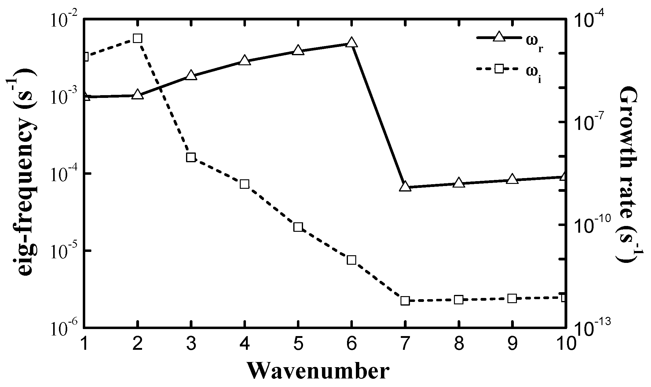
Based on the analytical and numerical methods mentioned above and the basic state of the structure, we can obtain the wave spectrum and all the eigenmode structures in Equation (15). Note that the basic-state vortex with hollow structure might be expected to set the stage for dynamic instability [2,15,35]. The hollow vortex as the basic state results in eigenvalues that are complex numbers (the real part represents the eigenfrequecy, and the image part represents the growth rate), indicating that the vortex system satisfies the condition of exponential instability. The eigenfrequecy and growth rate of the most unstable eigenmode (largest dimensionless growth rate) for azimuthal wavenumbers from 1 to 10 are displayed in Figure 2. It shows that the most unstable eigenmode for low wavenumber disturbances have greater growth rates with a magnitude of 10−5 s−1 at WN 1 and 2, and the growth rate of the most unstable mode at WN 2 is slightly larger with a value of 2.72 × 10⁻⁵ s−1. By definition [36], barotropic instability grows by extracting kinetic energy from the mean flow, therefore the initial instability can be seen as the most unstable mode (with the largest growth rate). Results of the experiment indicates that the WN2 is most unstable. The growth rate of the most unstable mode for high wavenumbers (3 waves or more) decay significantly, among which the growth rate of the most unstable mode at WN3 has been reduced to 10−9 in magnitude. Moreover, the growth rate of the most unstable mode for high wavenumbers larger than WN7 are only 10−13 in magnitude and their wave frequencies are less than 10−5 in magnitude. The eigenmodes with the growth rate less than 10−13 s−1 are regarded as neutral stable modes considering the influence of the numerical computation errors. Hence, the stability of the vortex system is mainly affected by low wavenumber disturbances.
It is well known that the intrinsic frequency of waves is one of the most important characteristics, and its magnitude can be used as an important criterion to judge the wave properties. Zhong and Zhang [20] examined the full spectrum of free waves on barotropic vortices. They propose the wave is higher-frequency associated with inertia-gravity waves (IGWs) when the intrinsic frequency is larger than the advective frequency (), while it may be low or intermediate frequency associated with either vortex Rossby waves (VRWs) or mixed vortex Rossby-inertio-gravity waves (VRIGWs) if the intrinsic frequency is between zero and the advective frequency or approach the advective frequency. Note that the eigenfrequency in this paper represents the Doppler-shifted frequency, namely,
where is the dimensional intrinsic frequency. So the intrinsic frequency can be estimated by the difference between the eigenfrequency and advective frequency. The intrinsic frequency from WN1 to WN6 lies between zero and the advective frequency, and the most unstable eigenmode belongs to higher frequency wave when the wavenumber is larger than 6. Totally, the instability of the hollow vortex in this paper is largely depends on low-intermediate frequency waves.
In this section, we examine the wave frequency and growth rate of the unstable eigenmodes for different azimuthal wavenumbers in the discretized system [Equations (12)–(14)] with the hollow vortex as the basic state. However, according to the basic principle of the above mode analysis method, it is necessary to obtain the weight coefficients of all eigenmodes in different azimuthal WNs to quantitatively describe the evolution characteristics of the unstable modes and their effects on the intensity and structural change of the basic-state vortex. Considering that the most unstable mode often represents the system evolution in the stage of linear development, we will mainly discuss the development characteristics of the disturbance at WN2.
3.2. Application of the Regularization Method
It is found that the rank of the 8999th order eigenmatrix X composed of all eigenvectors is 8998 in this paper, implying that this eigenmatrix is non-full rank under given basic-state vortex and resolution conditions. This would cause the process of solving the eigenmode weight coefficients to become ill-posed. Thus, it is necessary to introduce the Regularization method to solve this problem.
3.2.1. Determination of the Regularization Parameter
In this case, the initial wind field perturbation is set to zero, and we add a initial Gaussian geopotential height anomaly to the central area of the eyewall region following the approach of Nolan and Montgomery [32], which is expressed as:
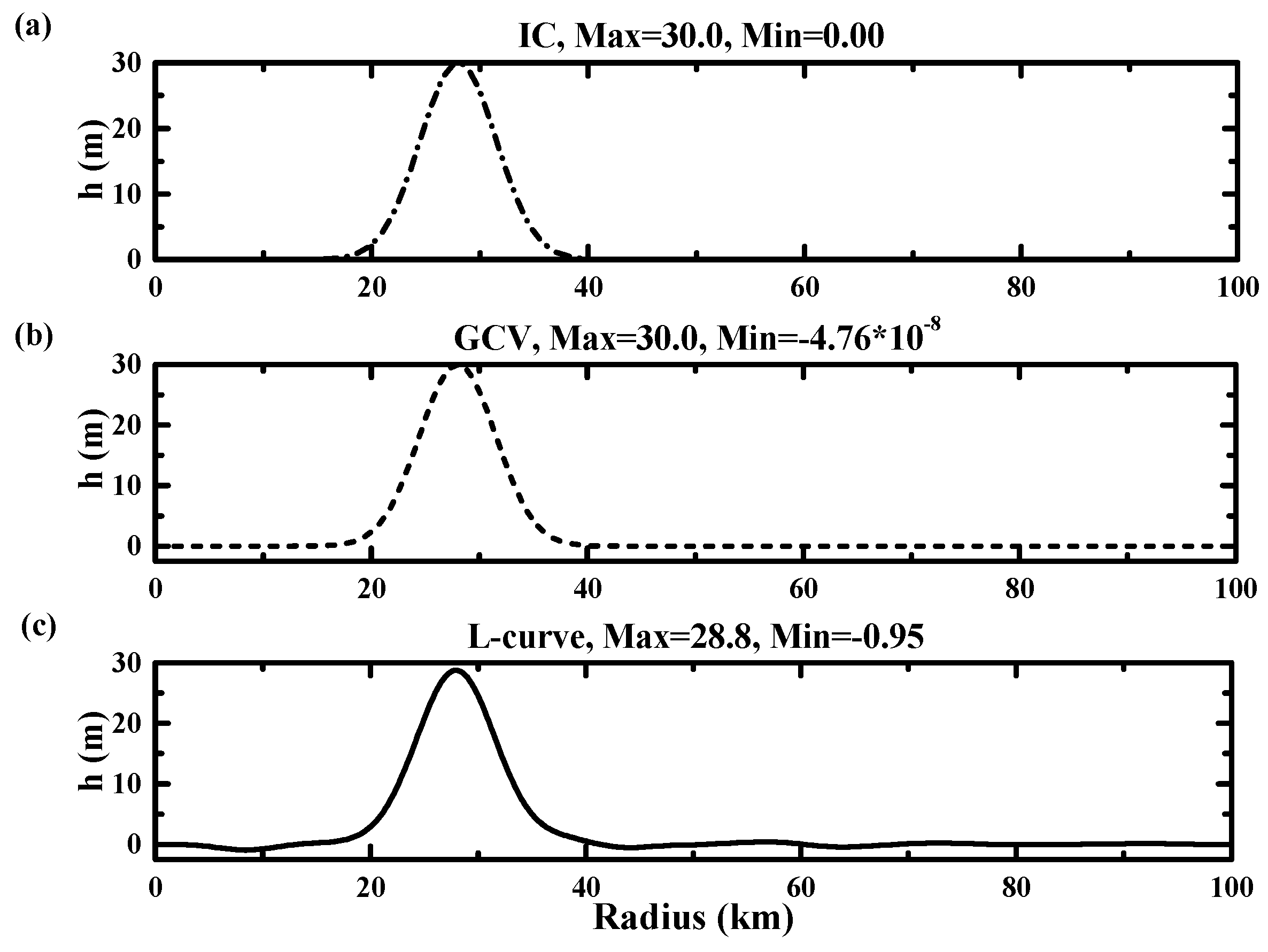
where reye = (r2 + r3)/2 is the center of the eyewall region, weye = r3 − r2 is the width of the eyewall region, and the initial amplitude of the perturbation is 1% of the resting depth, namely a = 0.01 × h0 here h0 = 3000 m. The maximum and the minimum of the initial disturbance is 30 m and zero, respectively. This initial perturbation is meant to be representative of the effect on the height field of an azimuthally localized burst of convection in the eyewall. Next, the GCV and L-curve methods are applied to solve the eigenmode coefficients for the ideal experiment, and the results are then used to calculate the initial height field by matrix inversion. The applicability of the two methods in the process of calculating the mode weight coefficients is analyzed by comparing the given initial condition and the inverse-calculated result.
The regularization parameters obtained by the two methods are 1.10 × 10⁻¹¹ and 5.82 × 10⁻⁴, respectively. Figure 3 shows the radial distribution of the initial height from the pre-specified initial condition and from the inverse calculation using two regulation methods. It is clear that the results of inverse calculation can well reproduce the Gaussian distribution of the pre-specified initial perturbation as well as the position and magnitude of the peak. However, structurally, the radial profile of perturbation height based on the GCV method is smoother and closer to the radial distribution of the given initial disturbance compared to that based on the L-curve method. Also, the maximum and minimum of the perturbation height with the GCV method are 30 m and −2.24 × 10⁻⁸ m, respectively, which are closer to that in the pre-specified initial disturbance, while the maximum and minimum based on the L-curve method are 28.8 m and −0.95, which have large errors. The above results indicate that the GCV method is more suitable than the L-curve method in this case. Thus, the regularization parameter obtained by the GCV method is determined to calculate the eigenmode weight coefficients in the inverse problem.
3.2.2. Distribution of the Mode Coefficients
Given initial perturbations and based on the eigen-matrix equations (Equation (15)), the regulation method can be used to examine the weight coefficients corresponding to each eigenmode at an azimuthal WN. The weight coefficients and the eigenmodes are one-to-one correspondence, thus the number of coefficients is closely related to the resolution of the numerical model. We set N = 3000, and a total of 3N − 1 eigenmodes. Hence, the corresponding number of coefficients is 8999. Note that the positive and negative coefficients only affect the phase of the mode structure, whereas the size of the weight of each individual eigenmode in the initial disturbance is determined by the absolute values of the coefficients. Next, we mainly focus on the distribution characteristics of the absolute values of the coefficients. The maximum and minimum absolute values of the eigenmode coefficients obtained in this case are 5.22 × 10⁷ and 3.83 × 10⁻¹², respectively, implying that large differences exist among the eigenmodes.
Based on Equation (19), it is obvious that the role of an eigenmode in the disturbance development is determined by its growth rate and corresponding weight coefficient in ELS method. The frequency shift is the same for positive and ngative eigenfrequencies and the shift is seen to increase with mode number. The 8999 eigenmodes in this case are sorted in a descending order by their growth rates to examine the role of different eigenmodes on the evolution of the vortex system. The higher the ranking is, the greater the growth rate is and more unstable the mode is. As an example, the first eigenmode corresponds to the largest growth rate and the most unstable mode. According to the mode ordering method mentioned above, the growth rates, eigenfrequencies and absolute values of weight coefficients of all eigenmodes for the most unstable WN (i.e., WN2) in this ideal experiment are shown in Figure 4. Since the positive (negative) growth rate directly denotes the development (damping) of the mode, these 8999 eigenmodes are displayed separately as the unstable modes (the first 2448 eigenmodes) and the damping modes (the rest of 6551 eigenmodes). As mentioned above, the unstable modes with the magnitude of growth rates less than 10−13 can be considered neutral and stable. These neutral modes (115 total) are ignored, and we only discuss the distribution characteristics of the remaining 2373 unstable modes.
Based on distributions of the coefficients for all eigenmodes (Figure 4e,f), it is apparent that there exist distinct differences ranging from 10−9 to 105 in coefficient magnitudes among these eigenmodes. As mentioned above, the role of an eigenmode in the system development is determined by the growth rate, which denotes the growth of perturbation amplitudes with time, and the weight coefficient, which represents the contribution of an eigenmode at the initial time. Thus, the role of a specific eigenmode can be different in the different stages of system development when taking into account the two influencing factors, although large differences are found in the growth rate of the eigenmodes.
In addition, the frequencies of the unstable modes are positive, implying that these unstable waves propagate clockwise relative to the basic state tangential flow, and the values of the eigenfrequencies are largely distributed within the range of [10−5, 10−2] s−1 (Figure 4c). These characteristics are highly consistent with the frequency and propagation characteristics of the VRWs and the mixed wave obtained by the wave theory and diagnostic analysis [1,2,4,31]. In contrast, the eigenfrequencies of the damping modes always pair with positive and negative values that cover a wide range including low, intermediate and high frequency ranges (Figure 4d). Moreover, the absolute values of the weight coefficients for the unstable modes are less than 1, much smaller than those for the damping modes, which are greater than 1000 (Figure 4e,f). The above results suggest that these damping modes mainly describe the high-frequency waves in which the energy in the synoptic system emits outward and disperses rapidly during a short time period. Although large differences exists in the coefficient distributions of various eigenmodes, large values of eigenfrequencies are mainly located in the middle and high frequency ranges corresponding to the damping modes that will decay rapidly and impose no great impacts on the system development. Therefore, the perturbation development is mainly affected by the unstable modes in this case. Note that the growth rates of the most unstable mode and the 2428th unstable mode are 7.97 × 10⁻⁶ s−1 and 1.38 × 10⁻¹⁶ s−1, respectively, and the difference in their magnitudes is above 10 orders, although the coefficient of the former (i.e., −14.5) is much smaller than that of the latter (i.e., 1.07 × 10⁴). After considering the two influencing factors, i.e., the growth rate and weight coefficient, it is not difficult to find that the most unstable mode still plays a leading role in the development of the disturbance. In the following, the obtained mode weight coefficients are applied to the mode linear superposition process to discuss the perturbation development.
3.2.3. The Results of the Mode Linear Superposition
The regularization method can solve the ill-posed problem occurred in the process of the computation of mode weight coefficients on the hollow vortex, which makes it practical to apply the ELS method for the study of the linear stability in vortices. Next we will discuss the evolution of the disturbance in the stage of linear instability and examine the role of a single wave on the perturbation development at an azimuthal WN based on the results of mode linear superposition.
Figure 5 compares the evolution of the radial perturbation wind between the most unstable mode multiplied by the corresponding weight coefficient (black lines) and all modes linearly superimposed (red lines) at WN 2. It is apparent that the disturbance based on mode linear superposition oscillates rapidly in the radial direction, and the amplitude of the oscillation gradually becomes smaller with time. It is shown that WN 2 disturbance undergoes an adjustment process in this stage, which is closely related to the rapid outward energy dispersion of high-frequency waves. However, the radial structure of the most unstable mode maintains a complete wave structure and the wave amplitude decreases gradually outward with radius. It is found that the oscillation of the disturbance has disappeared after an hour, and its radial structure is basically consistent, albeit with smaller magnitudes, as compared to the most unstable mode, implying that the dominant role of the most unstable mode is gradually emerging. The most unstable mode is almost exactly the same in the structure and magnitude as the results of mode linear superposition at 9 h. The radial perturbation wind has a magnitude of 100 ms−1, which is equivalent to the magnitude of the radial flow in real TCs. This indicates that the WN-2 disturbance is completely controlled by the most unstable mode, and the perturbation change caused by the mode development also is large enough to affect the structure and intensity change in the vortex system. The result is well consistent with the work of Menelaou et al. [22] based on the theory of empirical normal modes.
4. The Application of Mode Analysis in TC Dynamics
The main purpose of introducing the regularization method is to apply the ELS method t the TC dynamics study, especially the dynamics of the disturbance development in the linear instability stage. It provides an in-depth understanding of the internal dynamic mechanisms that affect intensity and structural change in TCs.
The disturbance characteristics corresponding to different wave numbers in TC have been discussed by using the Fourier decomposition method [39,40,41]. On the other hand, when the disturbance variables of the main WNs are linearly superimposed, the results can characterize the intensity and structure of the vortex system to a certain extent. The numerical integration results from WN1 to WN10 are selected and superimposed for each azimuthal WN. The results approximately represent the system intensity at each time and can be compared with the results of the most unstable mode based on the mode analysis approach.
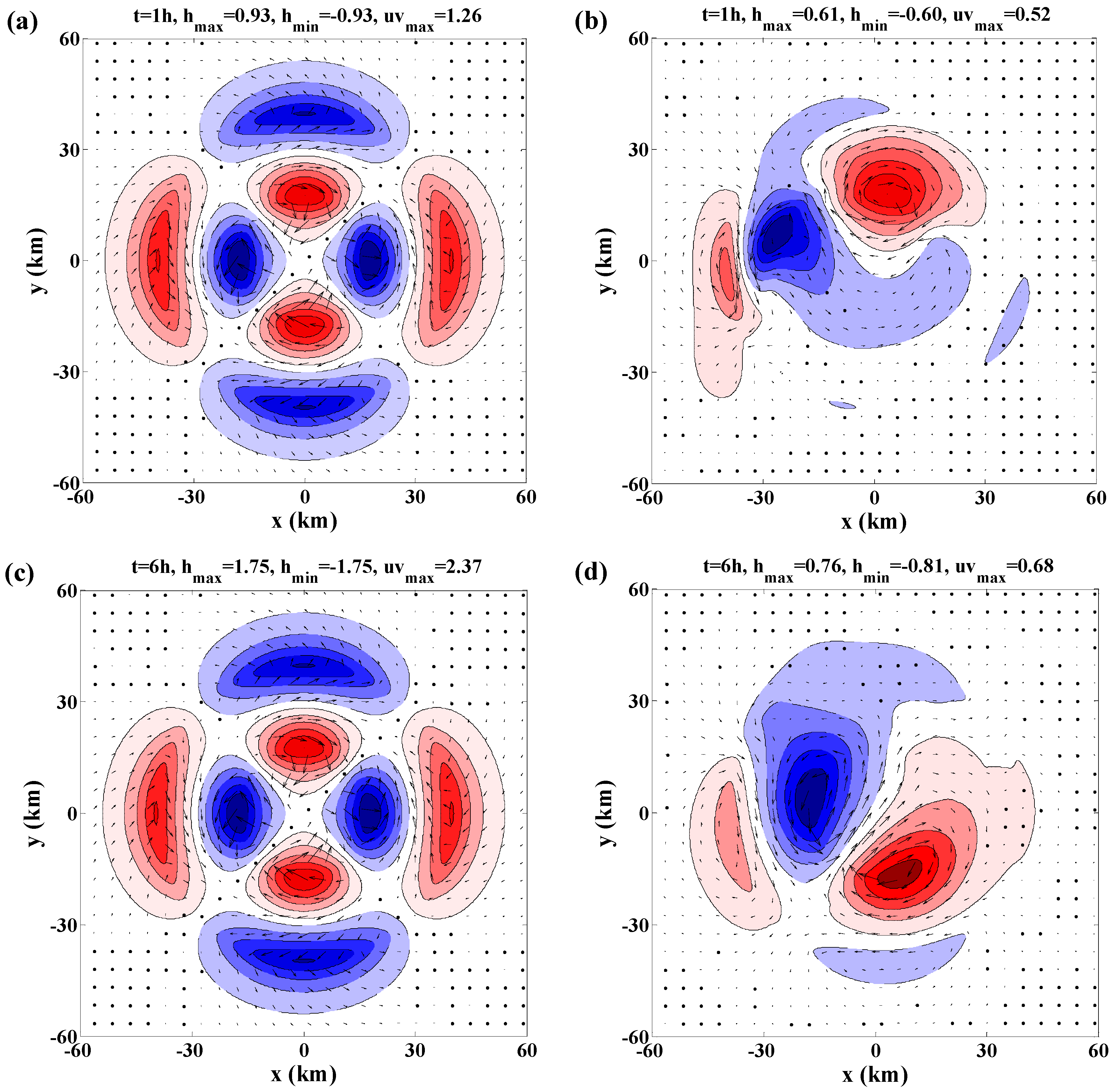
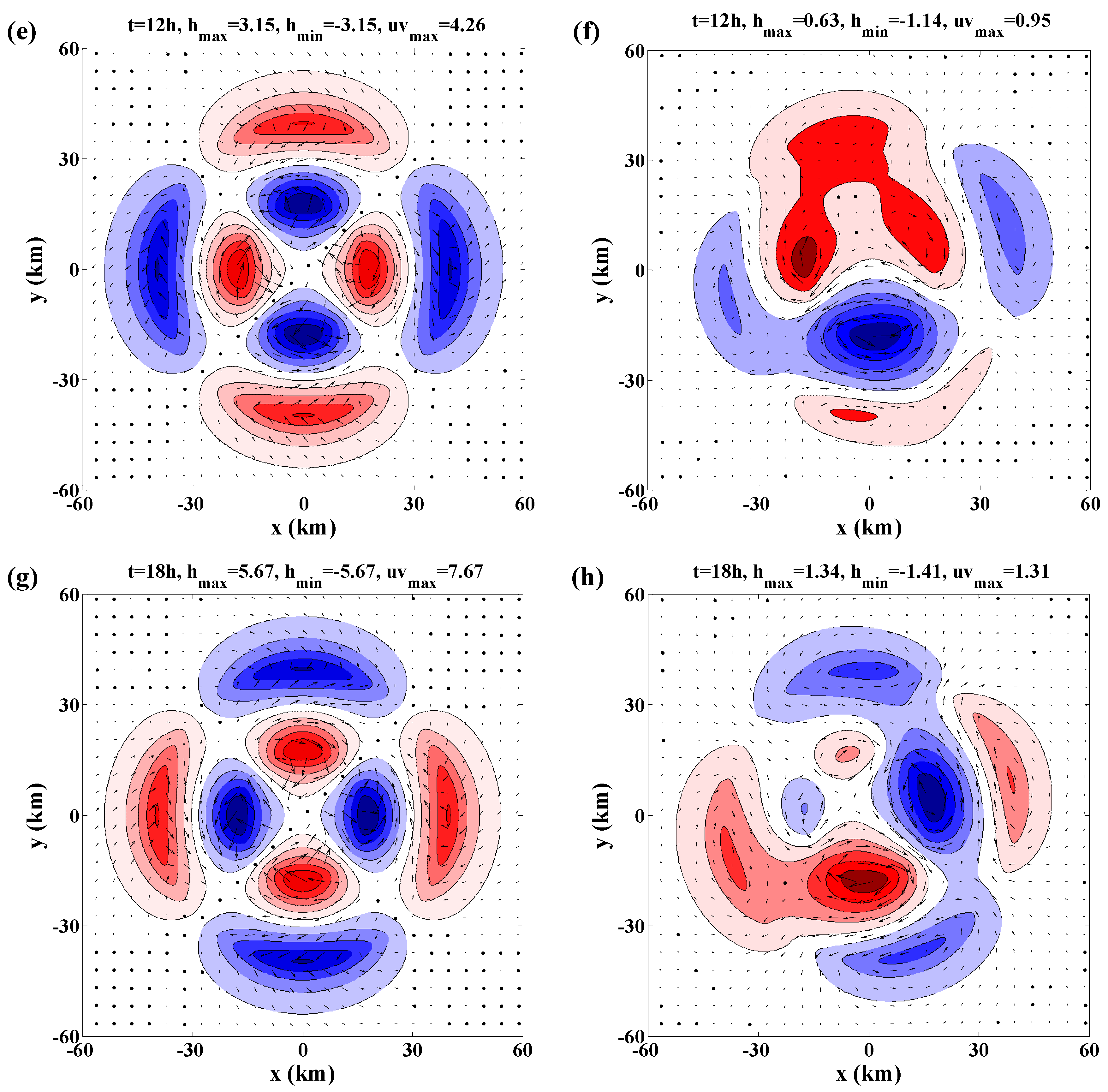
Figure 6 compares the evolution of perturbation height and horizontal flow vectors for WN2 based on results of the mode analysis and numerical integration approaches. The perturbation height of the most unstable mode has two distinct extremum regions, respectively located at the inner and outer edges of the eyewall, which consist of two symmetrical maximum centers and two symmetrical minimum centers that rotate along the tangential direction with the same angular velocity. It is found that the perturbation height is well correlated with wind vectors in the most unstable mode at WN2, with a higher (lower) free surface corresponding to clockwise (counter-clockwise) circulation. However, the wind vectors obviously move across the contours. Thus, the wave exhibits the typical characteristics of mixed VRIGWs [31]. The perturbation fields of the most unstable mode at WN2 gradually increase because of the presence of the dynamic instability, but the structures do not change. In contrast, the structure evolution of the system is more complicated in the early stage of disturbance development due to the common role of different WN disturbances obtained from the numerical integration approach. In the first 6 h, the disturbance mainly exhibits the characteristics of two positive centers and one negative center that alternately emerge in the inner-core region. The extreme centers with positive and negative staggered distribution gradually form in the inner and outer edges of the eyewall at t = 12 h as the disturbance continuously strengthens. The distinct large centers appear in the inner and outer edges of the eyewall at t = 18 h, showing a clear WN2 wave structure. In addition, the growing amplitude of the perturbation height in the first 18 h of integration is similar in magnitude to that of the most unstable mode, which increases by an order of magnitude from 10−1 to 100. This indicates that the disturbance development during this period is mainly affected by the dynamic instability. Since then, however, the growth rate of the disturbance significantly reduces. The maximum absolute value of the perturbation height is 6.05 at t = 30 h, while the eigen-variables of the most unstable mode still grows by at least one order of magnitude within 18 h with the maximum exceeding 33 m. The above results demonstrate that the disturbance development is also affected by other factors after integration of 18 h, while the role of unstable growth is no longer prominent. Apparently, a higher (lower) free surface corresponds to the clockwise (counter-clockwise) circulation, and wind vectors are mainly along the contour embodying a clear balanced characteristic. This is because the superposition of the numerical integration results for different WNs contains all types of waves that can affect the disturbance development. In summary, the disturbance development in the hollow vortex system is mainly affected by the dynamic instability, which is closely related to the most unstable mode for WN2. Moreover, it has been found that the wave structure of the most unstable mode has the characteristics of the mixed VRIGWs.
5. Conclusions
Previous studies [19,20] have confirmed that given initial perturbations, the eigenmode linear superposition (ELS) method can be used to examine the disturbance development at a certain azimuthal WN based on the linear dynamics. The ELS method is used to discuss the frequencies of the eigenmodes and the role of their instability in the intensity and structure change of the TC-like vortex, on the basis that the regularization approach has tackled the ill-posed problem occurred in analyzing the dynamic instability of the TC-like vortex by the ELS method.
In this study, the distribution characteristics of the instability as a function of wavenumbers for the basic state with the hollow vorticity ring are examined based on the linear barotropic shallow water equations. It is found that the disturbances for low wavenumbers are associated closely with the instability of the vortex system and eigenfrequencies correspond to the spectrum range within the coincidence between the frequencies of the VRWs and those of the mixed VRIGWs. The GCV method and L-curve method are used to determine the regularization parameters, which is the key to the regularization method. The radial distributions of the initial perturbation height obtained from the inversion results based on the two approaches are compared with the pre-specified initial perturbation height. It is found that the results of the GCV method are closer to the pre-specified initial condition in the solution of the inverse problem of the vortex system. Therefore, the GCV method is finally selected to solve the ill-posed problem with its regularization parameter α = 1.10 × 10⁻¹¹.
The frequency distribution, the growth rate and corresponding weight coefficient of various eigenmodes at the most unstable wavenumber are further discussed. Results show that the eigenmodes possessing large values of coefficients rapidly decay in the process of disturbance development and have little impact on the system development. Thereby, the above results indicate that the disturbance development is mainly affected by the unstable modes that is consistent with the results of mode linear superposition. The results of the ELS method show that the short-period obvious oscillation of perturbation variables appear along the radial direction in the early stage of disturbance development, which are closely related to the rapid outward energy dispersion of high-frequency waves. As the perturbation develops continuously, the dominant role of the most unstable mode in the disturbance development becomes more prominent. After a while, the most unstable mode is almost exactly the same in the structure and magnitude as the results of linear superposition of all eigenmodes. The magnitude of radial perturbation wind is equivalent to that of the radial flows in real TCs. This indicates that the WN2 disturbance is completely controlled by the most unstable mode, and its change caused by the mode superposition is large enough to affect the structure and intensity change of the vortex system.
Finally, the influence of the most unstable mode on the overall change of the hollow vortex is discussed by the product of the eigenfunction for the most unstable mode and its weight coefficient obtained from the regularization method. In the early stage of disturbance development (within integration of the first 18 h), the intensity and structure change are mainly affected by the dynamic instability, and the most unstable mode has a dominant role in the growth rate and the horizontal distribution of intense disturbance in the near-core region. Moreover, it has been found that the wave structure of the most unstable mode possesses typical characteristics of mixed VRIGWs.
In conclusion, the regularization method can effectively solve the ill-posed problem appearing in eigenmode linear superposition. The ELS method provides a new research idea for understanding the dynamic mechanism that impacts intensity and structural change of TCs. In the future, we will continue to use the ELS method to further study waves and their stability in TCs.
Acknowledgments
The research was supported by the National Natural Science Foundation of China (41275002), the National Natural Science Foundation of China (41175089), the National Natural Science Foundation of China (41475021), the National Natural Science Foundation of China (41775055), and the State Key Program of National Natural Science Foundation of China (41230421).
Author Contributions
Wei Zhong conceived and designed the experiments; Shuang Liu performed the experiments; Wei Zhong and Shuang Liu analyzed the data; Yudi Liu and Jie Xiang contributed analysis tools; Shuang Liu wrote the paper.
Conflicts of Interest
The authors declare no conflict of interest.
References
- Montgomery, M.T.; Kallenbach, R.J. A theory for vortex Rossby-waves and its application to spiral bands and intensity changes in hurricanes. Q. J. R. Meteorol. Soc. 1997, 123, 435–465. [Google Scholar] [CrossRef]
- Schubert, W.H.; Montgomery, M.T.; Taft, R.K.; Guinn, T.A.; Fulton, S.R.; Kossin, J.P.; Edwards, J.P. Polygonal eyewalls, asymmetric eye contraction, and potential vorticity mixing in hurricanes. J. Atmos. Sci. 1999, 56, 1197–1223. [Google Scholar] [CrossRef]
- Wang, Y. Vortex Rossby waves in a numerically simulated tropical cyclone. Part I: Overall structure, potential vorticity, and kinetic energy budgets. J. Atmos. Sci. 2002, 59, 1213–1238. [Google Scholar] [CrossRef]
- Wang, Y. Vortex Rossby waves in a numerically simulated tropical cyclone. Part II: The role in tropical cyclone structure and intensity changes. J. Atmos. Sci. 2002, 59, 1239–1262. [Google Scholar] [CrossRef]
- Schecter, D.A.; Montgomery, M.T. Damping and pumping of a vortex Rossby wave in a monotonic cyclone: Critical layer stirring versus inertia-buoyancy wave emission. Phys. Fluids 2004, 16, 1334–1348. [Google Scholar] [CrossRef]
- Schecter, D.A.; Montgomery, M.T. Conditions that inhibit the spontaneous radiation of spiral inertia–gravity waves from an intense mesoscale cyclone. J. Atmos. Sci. 2006, 63, 435–456. [Google Scholar] [CrossRef]
- Schecter, D.A. The spontaneous imbalance of an atmospheric vortex at high Rossby number. J. Atmos. Sci. 2008, 65, 2498–2521. [Google Scholar] [CrossRef]
- Montgomery, M.T.; Nicholls, M.E.; Cram, T.A.; Saunders, A. A vortical hot tower route to tropical cyclogenesis. J. Atmos. Sci. 2006, 63, 355–386. [Google Scholar] [CrossRef]
- Nguyen, S.; Smith, R.; Montgomery, M.T. Tropical-cyclone intensification and predictability in three dimensions. Q. J. R. Meteorol. Soc. 2008, 134, 563–582. [Google Scholar] [Green Version]
- Moller, J.; Montgomery, M.T. Vortex Rossby waves and hurricane intensification in a barotropic model. J. Atmos. Sci. 1999, 56, 1674–1687. [Google Scholar] [CrossRef]
- Moller, J.; Montgomery, M. Tropical cyclone evolution via potential vorticity anomalies in a three-dimensional balance model. J. Atmos. Sci. 2000, 57, 3366–3387. [Google Scholar] [CrossRef]
- Nolan, D.S.; Montgomery, M.T. Nonhydrostatic, three-dimensional perturbations to balanced, hurricane-like vortices. Part I: Linearized formulation, stability, and evolution. J. Atmos. Sci. 2002, 59, 2989–3020. [Google Scholar] [CrossRef]
- Kossin, J.P.; Eastin, M.D. Two distinct regimes in the kinematic and thermodynamic of the hurricane eye and eyewall. J. Atmos. Sci. 2001, 58, 1079–1090. [Google Scholar] [CrossRef]
- Menelaou, K.; Yau, M.K.; Martinez, Y. On the dynamics of the secondary eyewall genesis in Hurricane Wilma (2005). Geophys. Res. Lett. 2012, 39, L04801. [Google Scholar] [CrossRef]
- Montgomery, M.T.; Shapiro, L.J. Generalized CharneyStern and Fjørtoft theorems for rapidly rotating vortices. J. Atmos. Sci. 1995, 52, 1829–1833. [Google Scholar] [CrossRef]
- Rozoff, C.M.; Kossin, J.P.; Schubert, W.H.; Mulero, P.J. Internal control of hurricane intensity: The dual nature of potential vorticity mixing. J. Atmos. Sci. 2009, 66, 133–147. [Google Scholar] [CrossRef]
- Hendricks, E.A.; Schubert, W.H.; Taft, R.K.; Wang, H.; Kossin, J.P. Life cycles of hurricane-like vorticity rings. J. Atmos. Sci. 2009, 66, 705–722. [Google Scholar] [CrossRef]
- Schecter, D.A.; Dubin, D.H.E.; Cass, A.C.; Driscoll, C.F.; Lansky, I.M.; O’Neil, T.M. Inviscid damping of asymmetries on a two-dimensional vortex. Phys. Fluids 2000, 12, 2397. [Google Scholar] [CrossRef]
- Montgomery, M.T.; Lu, C. Free waves on barotropic vortices. Part I: Eigenmode structure. J. Atmos. Sci. 1997, 54, 1868–1885. [Google Scholar] [CrossRef]
- Zhong, W.; Zhang, D.L. An Eigenfrequency Analysis of Mixed Rossby–Gravity Waves on Barotropic Vortices. J. Atmos. Sci. 2014, 71, 2186–2203. [Google Scholar] [CrossRef]
- Martinez, Y.H.; Brunet, G.; Yau, M.K. On the dynamics of 2D hurricane-like vortex symmetrization. J. Atmos. Sci. 2010, 67, 3559–3580. [Google Scholar] [CrossRef]
- Menelaou, K.; Yau, M.K.; Martinez, Y. Impact of asymmetric dynamical processes on the structure and intensity change of two-dimensional hurricane-like annular vortices. J. Atmos. Sci. 2013, 70, 559–582. [Google Scholar] [CrossRef]
- Flatau, M.; Stevens, D.E. Barotropic and inertial insta-bilities in the hurricane outflow layer. Geophys. Astrophys. Fluid Dyn. 1989, 47, 1–18. [Google Scholar] [CrossRef]
- Nolan, D.S.; Montgomery, M.T.; Grasso, L.D. The wavenumber-one instability and trochoidal motion of TC-like vortices. J. Atmos. Sci. 2001, 58, 3243–3270. [Google Scholar] [CrossRef]
- Tikhonov, A.; Arsenin, V. Solutions to Ill-Posed Problems; V. H. Winston & Sons: Washington, DC, USA, 1977; p. 491. [Google Scholar]
- Shen, Y.Z.; Xu, H. Spectral decomposition formula of regularization solution for ill-posed equation. J. Geod. Geodyn. 2002, 22, 10–14. (In Chinese) [Google Scholar] [CrossRef]
- Zhou, J.W.; Ou, J.K. On alteration of quasi-stable points and some problems concerning free net adjustment. Acta Geod. Cartogr. Sin. 1984, 13, 161–170. (In Chinese) [Google Scholar]
- Tikhonov, A.N. On the solution of incorrectly posed problem and the method of regularization. Sov. Math. 1963, 4, 1035–1038. [Google Scholar]
- Phillips, D.L. A technique for the numerical solution of certain integral equations of the first kind. J. Assoc. Comput. Mach. 1962, 9, 84–97. [Google Scholar] [CrossRef]
- Golub, G.H.; Heath, M.; Wahba, G. Generalized cross-validation as a method for choosing a good ridge parameter. Technometrios 1979, 21, 215–223. [Google Scholar] [CrossRef]
- Hansen, P.C.; O’Leary, D.P. The use of the L-curve in the regularization of discrete ill-posed problems. SIAM J. Sci. Comput. 1993, 14, 1487–1503. [Google Scholar] [CrossRef]
- Nolan, D.S.; Montgomery, M.T. The algebraic growth of wavenumber one disturbances in hurricane-like vorticies. J. Atmos. Sci. 2000, 57, 3514–3538. [Google Scholar] [CrossRef]
- Zhong, W.; Zhang, D.L.; Lu, H.C. A theory for mixed vortex Rossby-gravity waves in tropical cyclones. J. Atmos. Sci. 2009, 66, 3366–3381. [Google Scholar] [CrossRef]
- Zhong, W.; Lu, H.C.; Zhang, D.L. Mesoscale barotropic instability of vortex Rossby waves in tropical cyclones. Adv. Atmos. Sci. 2010, 27, 243–252. [Google Scholar] [CrossRef]
- Kossin, J.P.; Schubert, W.H. Mesovortices, polygonal flow patterns, and rapid pressure falls in hurricane-like vortices. J. Atmos. Sci. 2001, 58, 2196–2209. [Google Scholar] [CrossRef]
- Hendricks, E.A. Tropical Cyclone Evolution via Internal Asymmetric Dynamics. Ph.D. Thesis, Colorado State University, Fort Collins, CO, USA, 2008; 150p. [Google Scholar]
- Hendricks, E.A.; Schubert, R.K.; Chen, Y.H. Hurricane eyewall evolution in a forced shallow-water model. J. Atmos. Sci. 2014, 71, 1623–1643. [Google Scholar] [CrossRef]
- Liu, S.; Zhong, W.; Lu, H.C.; Liu, J.C. The contribution of structure and evolution of potential vorticity tower to the intensity change of Hurricane Wilma (2005). Chin. J. Geophys. 2015, 58, 1513–1525. (In Chinese) [Google Scholar] [CrossRef]
- Boyd, J.P. Chebyshev and Fourier Spectral Methods; Courier Corporation Press: Mineola, NY, USA, 2001; 689p. [Google Scholar]
- Lonfat, M.; Chen, S.S.; Mark, F.D. Precipitation distribution in tropical cyclones using the Tropical Rainfall Measuring Mission (TRMM) microwave imager: A global perspective. Mon. Weather Rev. 2004, 132, 1645–1660. [Google Scholar] [CrossRef]
- Yang, L.; Fei, J.-F.; Huang, X.-G. Asymmetric distribution of convection in tropical cyclones over the Western North Pacific Ocean. Adv. Atmos. Sci. 2016, 33, 1306–1321. [Google Scholar] [CrossRef]
Figure 1.
Radial distribution of (a) relative vorticity (10−3 s−1); (b) azimuthal velocity (ms−1); (c) angular velocity (10−3 s−1); (d) fluid depth (km) with a hollow vortex as the basic state.
Figure 1.
Radial distribution of (a) relative vorticity (10−3 s−1); (b) azimuthal velocity (ms−1); (c) angular velocity (10−3 s−1); (d) fluid depth (km) with a hollow vortex as the basic state.
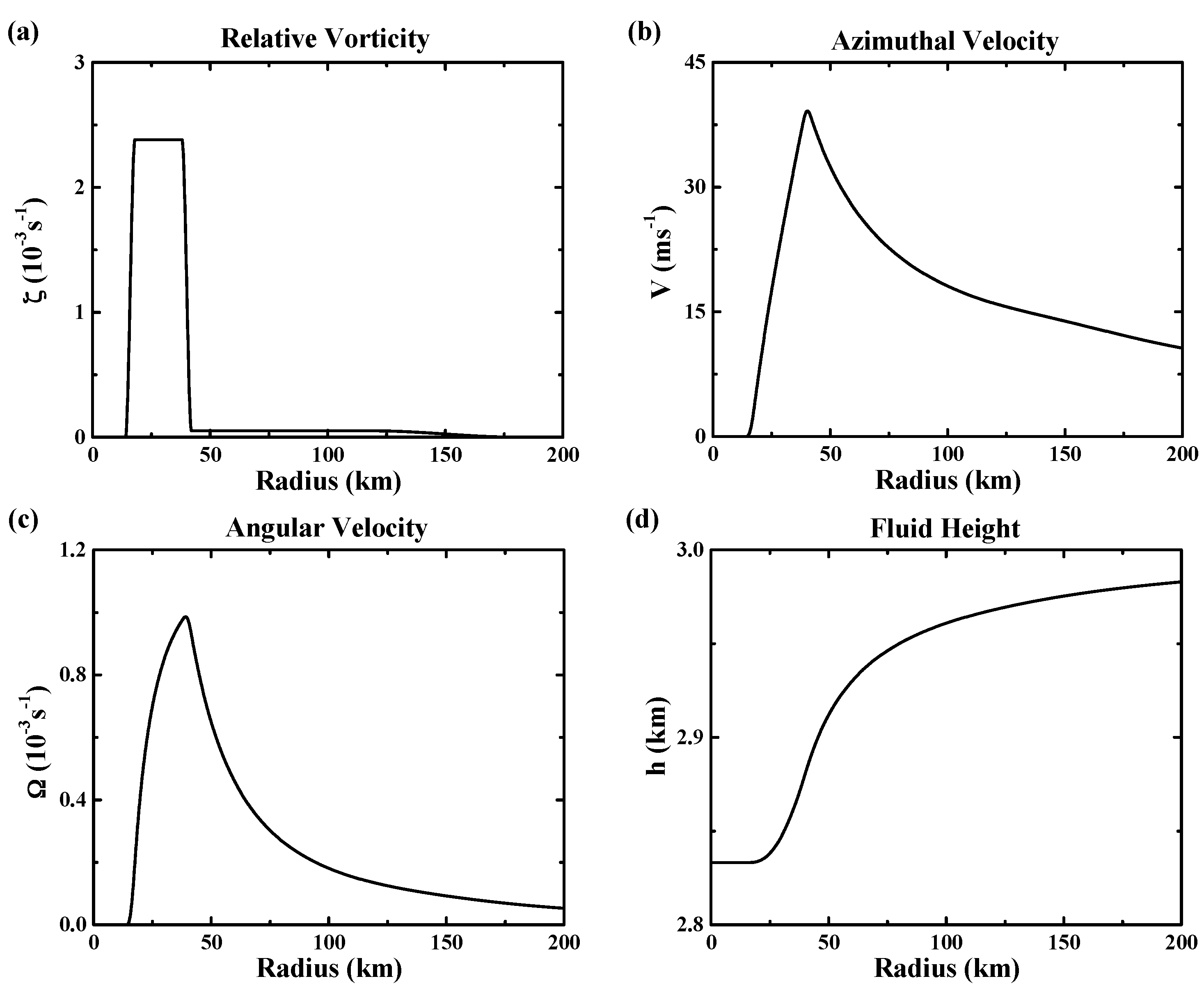
Figure 2.
The eigenfrequencies (solid line) and the growth rates (dash line) of the most unstable mode as a function of azimuthal WN (n = 1–10) in association with the hollow vortex in Figure 1.
Figure 2.
The eigenfrequencies (solid line) and the growth rates (dash line) of the most unstable mode as a function of azimuthal WN (n = 1–10) in association with the hollow vortex in Figure 1.

Figure 3.
Radial distributions of the perturbation height at initial time: (a) the result of the given initial condition; (b) the inverse result based on the GCV method; (c) the inverse result based on the L-curve method.
Figure 3.
Radial distributions of the perturbation height at initial time: (a) the result of the given initial condition; (b) the inverse result based on the GCV method; (c) the inverse result based on the L-curve method.

Figure 4.
The unstable modes and the damping modes at WN 2, correspond to the scatterplots of (a); (b) growth rate; (c,d) eigenfrequency; and (e,f) the absolute values of weight coefficients.
Figure 4.
The unstable modes and the damping modes at WN 2, correspond to the scatterplots of (a); (b) growth rate; (c,d) eigenfrequency; and (e,f) the absolute values of weight coefficients.
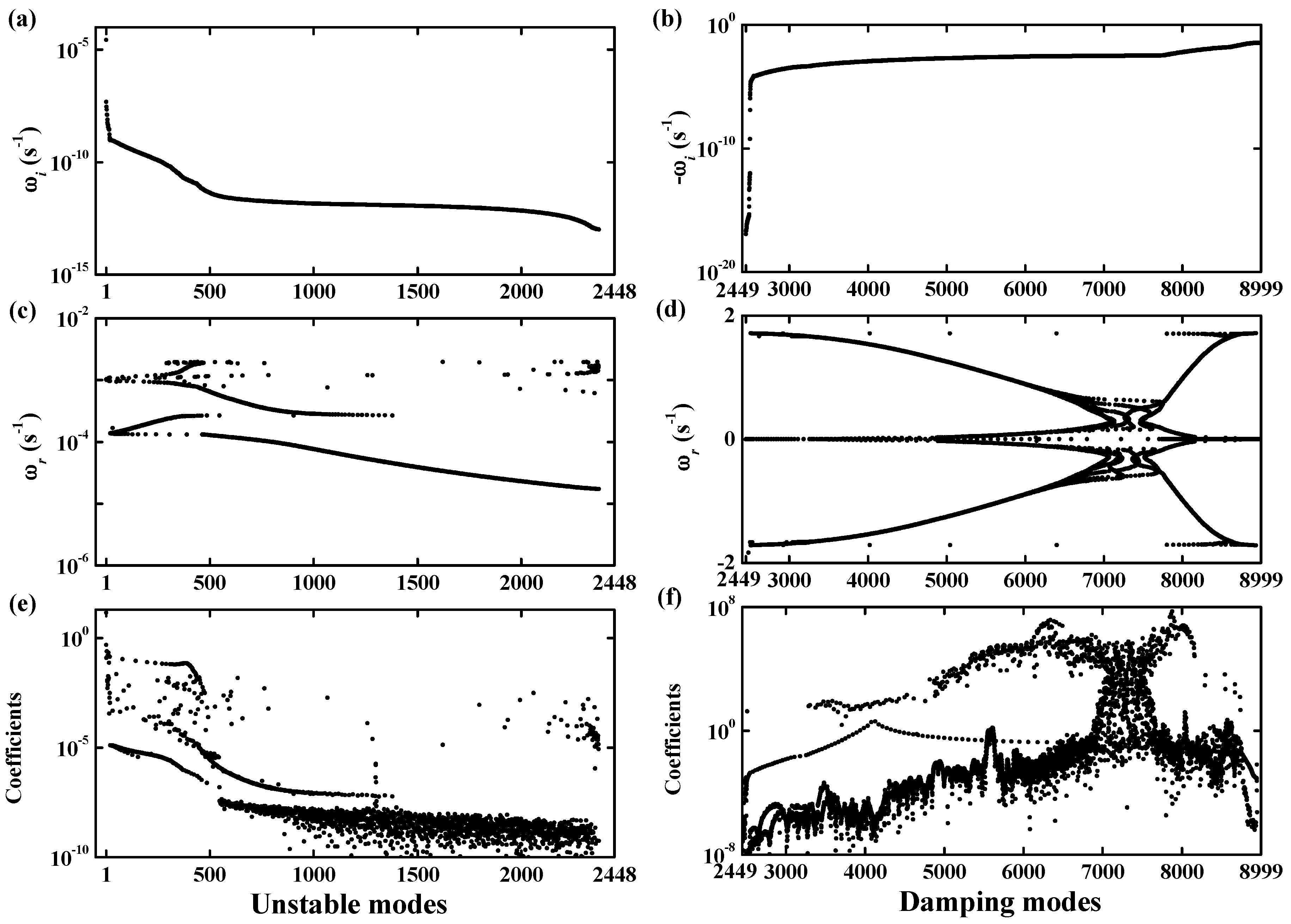
Figure 5.
The evolution of the radial perturbation wind obtained from the most unstable mode (black lines) and the linear-superimposed all eigenmodes (red lines). (a) the integration time from 0.5–2 h; (b) the integration time from 3–12 h; (c) the integration time from 15–24 h.
Figure 5.
The evolution of the radial perturbation wind obtained from the most unstable mode (black lines) and the linear-superimposed all eigenmodes (red lines). (a) the integration time from 0.5–2 h; (b) the integration time from 3–12 h; (c) the integration time from 15–24 h.
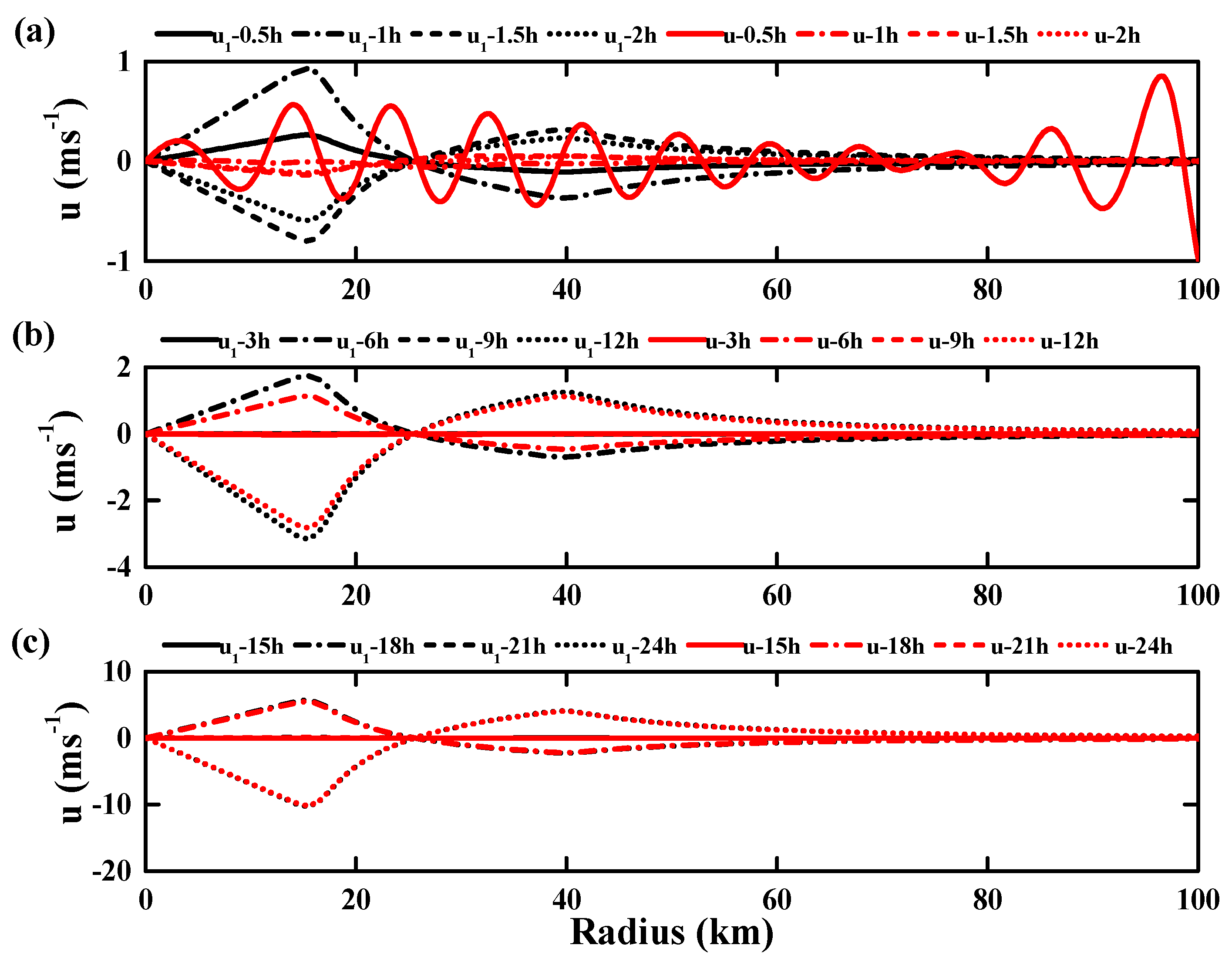
Figure 6.
The evolution of perturbation height (m; shaded, red is positive and blue is negative) and horizontal flow vectors (ms−1) obtained from (a,c,e,g) the most unstable mode and (b,d,f,h) superposition of the numerical integration results for different azimuthal WNs at t = 1 h, t = 6 h, t = 12 h and t = 18 h.


Table 1.
Parameters for the basic state relative vorticity profile.
| Parameter | ζ1 (s−1) | ζ2 | ζ3 | r1 (km) | r2 | r3 | r4 | r5 | r6 |
|---|---|---|---|---|---|---|---|---|---|
| value | 0.0 | 1.68 × 10⁻³ | 1.0 × 10⁻⁴ | 14 | 18 | 38 | 42 | 120 | 180 |
© 2018 by the authors. This article is an open access article distributed under the terms and conditions of the Creative Commons Attribution license (http://creativecommons.org/licenses/by/4.0/).
Share and Cite
MDPI and ACS Style
Liu, S.; Zhong, W.; Liu, Y.; Xiang, J. An Analysis of Dynamic Instability on TC-Like Vortex Using the Regularization-Based Eigenmode Linear Superposition Method. Atmosphere 2018, 9, 26. https://doi.org/10.3390/atmos9010026
AMA Style
Liu S, Zhong W, Liu Y, Xiang J. An Analysis of Dynamic Instability on TC-Like Vortex Using the Regularization-Based Eigenmode Linear Superposition Method. Atmosphere. 2018; 9(1):26. https://doi.org/10.3390/atmos9010026
Chicago/Turabian StyleLiu, Shuang, Wei Zhong, Yudi Liu, and Jie Xiang. 2018. "An Analysis of Dynamic Instability on TC-Like Vortex Using the Regularization-Based Eigenmode Linear Superposition Method" Atmosphere 9, no. 1: 26. https://doi.org/10.3390/atmos9010026
Note that from the first issue of 2016, this journal uses article numbers instead of page numbers. See further details here.