1. Introduction
The societal impact of fog has significantly increased during the modern era, mainly as a hindrance to marine, air and road traffic. In industrial regions, fog also greatly impacts air quality: air pollutants from combustion processes can dissolve in fog water particles, generating toxic acids that can damage various surfaces and cause fatal diseases when inhaled. Furthermore, the tops of fog layers reflect solar radiation, which reduces air exchange fluxes when temperature inversions are present [
1]. In contrast to these negative effects, fog is often considered as a positive element in hydrology as it can supply otherwise arid ecosystems with moisture [
2,
3].
Operational spatio-temporal observation is hampered by the sparse density of existing observation networks, especially in complex terrain [
4,
5]. To tackle this problem, different methods for operational fog forecasting and nowcasting have been developed in the past (see Gultepe et al. [
6] for an overview). A major problem with numerical models is the uncertainty in the parameterization of turbulence and microphysical processes, as the processes involved are not fully understood and there is a lack of empirical data that could provide better information [
7]. One problem with satellite-based nowcasting methods is the reliable distinction between ground fog and low stratus layers [
8]. Bendix et al. [
9] and Cermak and Bendix [
10] used (sub)adiabatic approximations of the vertical liquid water content (LWC) profile to retrieve cloud thickness, which, in turn, was used for the distinction between ground fog and low stratus layers. The approximations can lead to inaccuracies, however, as computed cloud thickness is highly sensitive to the assumed LWC profile and the integrated liquid water path (LWP) [
10].
Many of the above-mentioned methods would largely benefit from information about the vertical distribution of LWC with a high temporal resolution over the whole fog life cycle. Unfortunately, few data are available concerning the LWC for complete fog events, as well as for single fog life cycle stages. Airborne measurements are impossible due to the narrow vertical profile of fog. Balloon-borne systems are also unsuitable for continuous measurement of the vertical fog structure. One possible solution comprises millimeter-wavelength cloud radars that could provide continuous LWC measurements in a high temporal resolution [
4,
11]. Especially radars using the frequency-modulated continuous wave technique (FMCW) are able to provide measurements of very low fog layers due to their small near-field of about 30 m [
4,
12].
Reliable Z-LWC relationships for fog events are paramount to retrieving LWC profiles from radar reflectivity (Z). Existing procedures use empirically-derived static relationships that do not account for different fog types, vertical drop size distribution (DSD) differences or life cycle stages, e.g., [
13,
14,
15,
16]. More advanced methods try to compensate for these shortcomings by including additional instrumentation, e.g., LiDAR ceilometers [
17] or a combination of passive and active microwave profilers [
18], and by considering the effect of different DSDs. However, assumptions about the shape of the DSD (e.g., lognormal or gamma distributed, temporally-fixed DSD) and/or the droplet concentration (fixed total drop count
) also lead to inaccuracies in retrieved Z-LWC relationships [
18,
19]. This is due to the fact that Z is proportional to the sixth moment of the DSD while LWC is proportional to the third moment of the DSD. Therefore, variations in the DSD strongly influence the Z-LWC relationship [
4,
20].
Concerning the high temporal dynamics of fogs, such assumptions about the DSD are not suitable for a proper retrieval of LWC from Z. Several authors have identified different evolutionary stages with a strong influence on DSD, and thus, the relationship between Z and LWC (e.g., [
21,
22,
23,
24]). As the variability of the droplet spectrum is a function of the development stage, taking the development stages associated with the nebular dynamics into consideration thus forms the essential basis for deriving the LWC profile more reliably [
20,
25]. In a sensitivity study, Maier et al. [
4] showed that there is a direct, but nonlinear relationship between Z and LWC, which can be described by specific DSD characteristics according to the fog life cycle stage. Maier et al. [
4] differentiated different life cycle stages during radiation fog events by means of the measured DSD.
In the present study, the temporal variability of DSD and its influence on the Z-LWC relationship were investigated for radiation fog events using data obtained at the Marburg Ground Truth and Profiling Station in Linden-Leihgestern, Germany. This study tested whether (1) different fog life cycle stages show significantly different DSD, (2) a characteristic DSD can be identified for each life cycle stage and (3) it is possible to derive reliable Z-LWC relationships by means of the assigned characteristic DSD. If the study questions can be affirmed, a next logical step could be to investigate the vertical variation of the DSD over the whole fog life cycle. By means of a balloon-borne measurement platform, it would then be possible to determine if a vertical stratification of the fog layer exists as stated, e.g., by Cermak and Bendix [
10], and if there is a relationship between the vertical DSDs and the ground-measured DSDs with respect to the identified development stages. Based on such relationships, the ground-based DSD measurements could be used to retrieve Z-LWC equations applicable to the reflectivity profile of cloud radars. Using balloon-borne DSD measurements, Egli et al. [
26] investigated the LWC profile during two fog events in 2011 and 2012 at the Marburg Ground Truth and Profiling Station. No indication for a vertical dependency of the DSD parameters was identified based on the limited dataset. However, the variability within the measurements suggested that more DSD profiles during a variety of different fog events should be collected for a more representative investigation of the vertical and temporal dependency of the DSD profiles.
Reliable Z-LWC relationships based on DSD information could be applied to our 94 GHz FMCW cloud radar profiler in Linden-Leihgestern. The millimeter-wavelength makes it highly sensitive to cloud and fog droplets, while the signal attenuation in the relevant atmospheric range is relatively low. Furthermore, the maximum temporal resolution of 10 s, the maximum vertical resolution of 4 m and the minimal height of the reflectivity profile of 30 m make it very suitable to investigate fog properties. The continuously-retrieved LWC profiles would be very helpful to understand fog dynamics in general and to improve satellite-based fog detection schemes, as well as numerical fog modeling approaches.
The article is structured as follows:
Section 2 gives an overview of the instruments used, the fog data acquired and the processing steps.
Section 3 presents the results, which are then discussed in
Section 4. A conclusion and a short outlook are given in
Section 5. A theoretical background concerning the Z-LWC relationships can be found in the
Appendix A.
3. Results
The following section presents findings in regards to the temporal variability of DSD and its influence on the Z-LWC relationship. First, the different fog life cycle stages are checked for significantly different DSD characteristics. Next, we investigate if characteristic DSDs can be identified for the life cycle stages. Finally, we examine the possibility of deriving reliable Z-LWC relationships by means of a characteristic DSD.
3.1. Visual Analysis of DSD Differences for Different Fog Life Cycle Stages
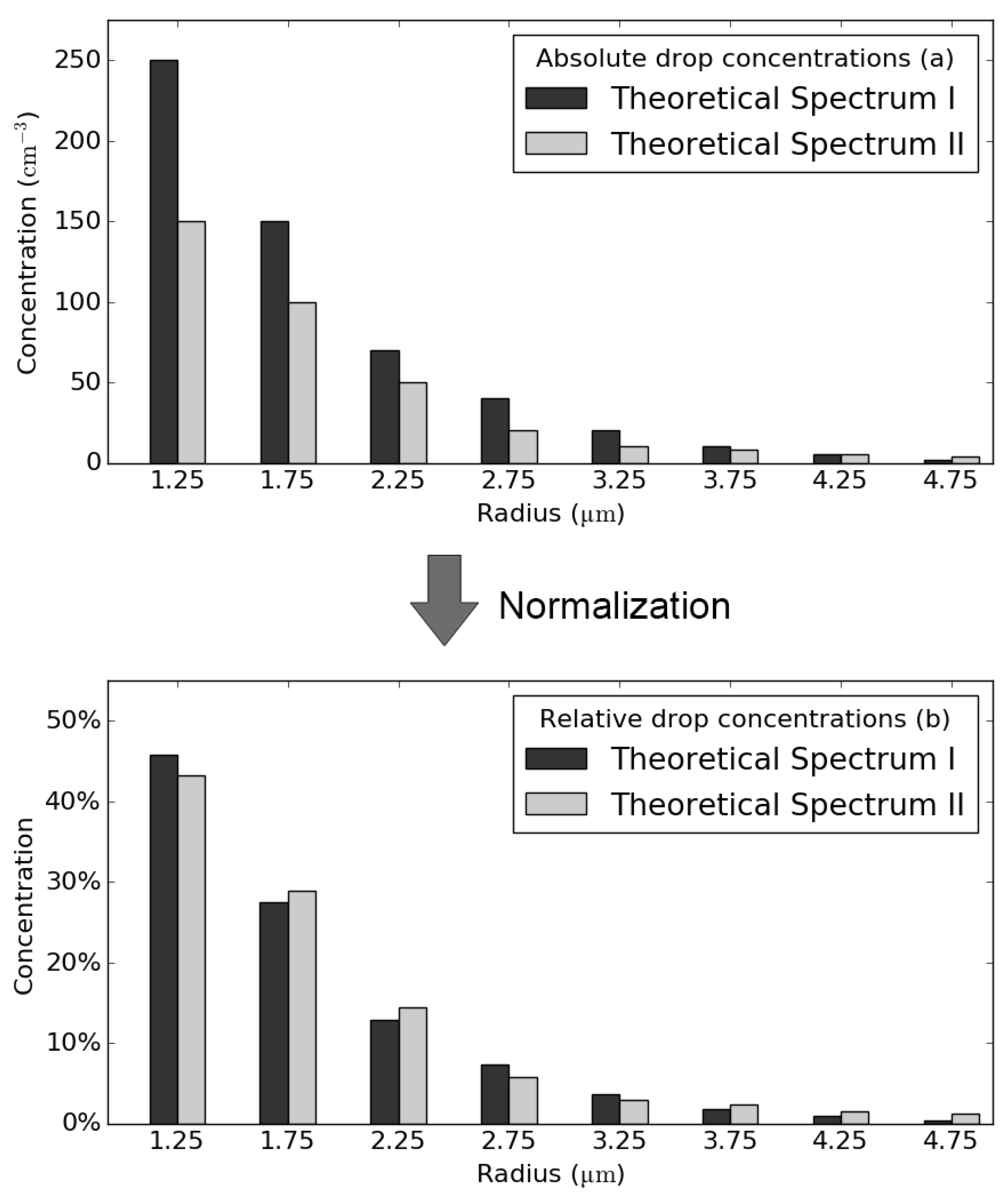
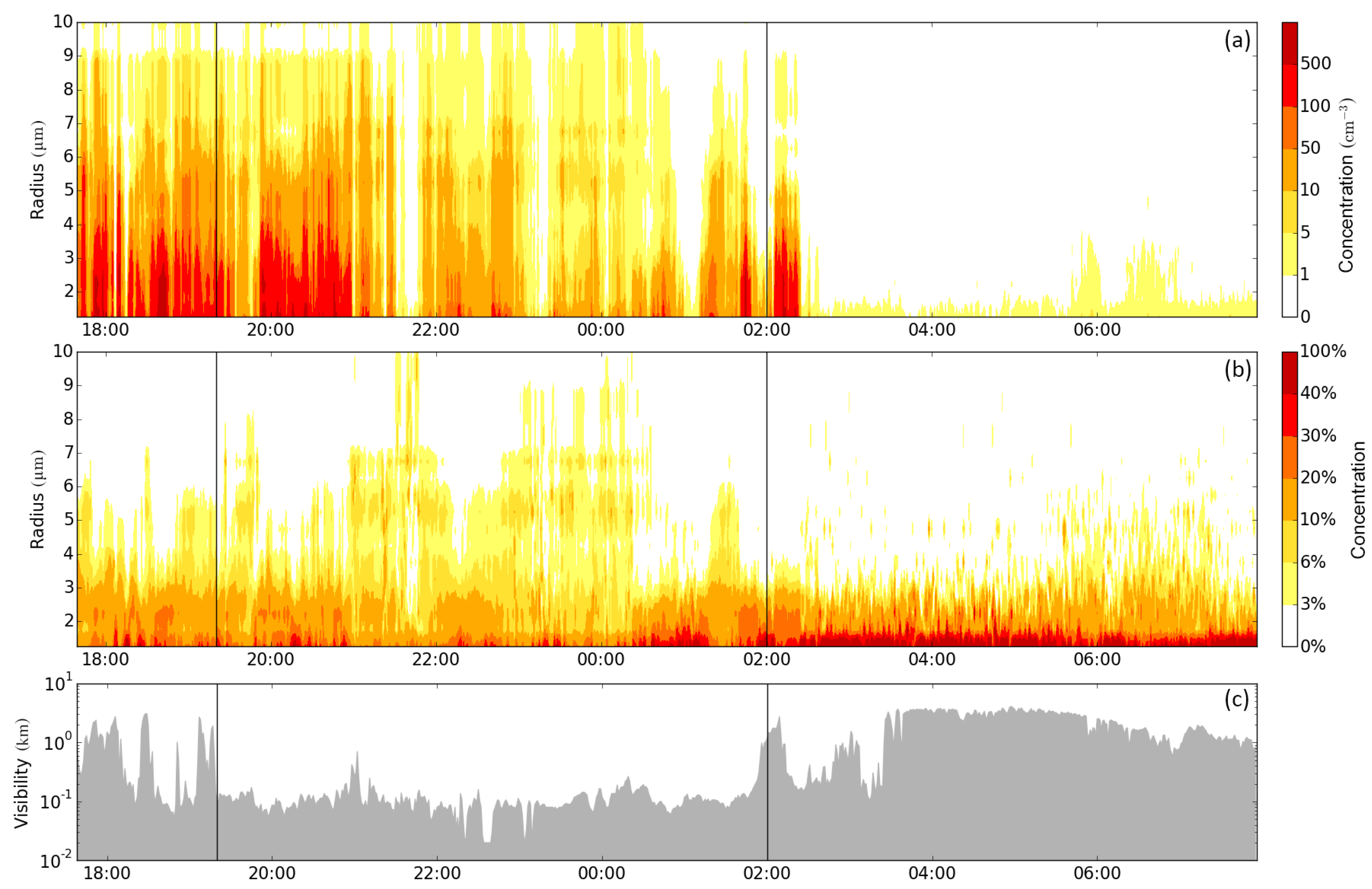
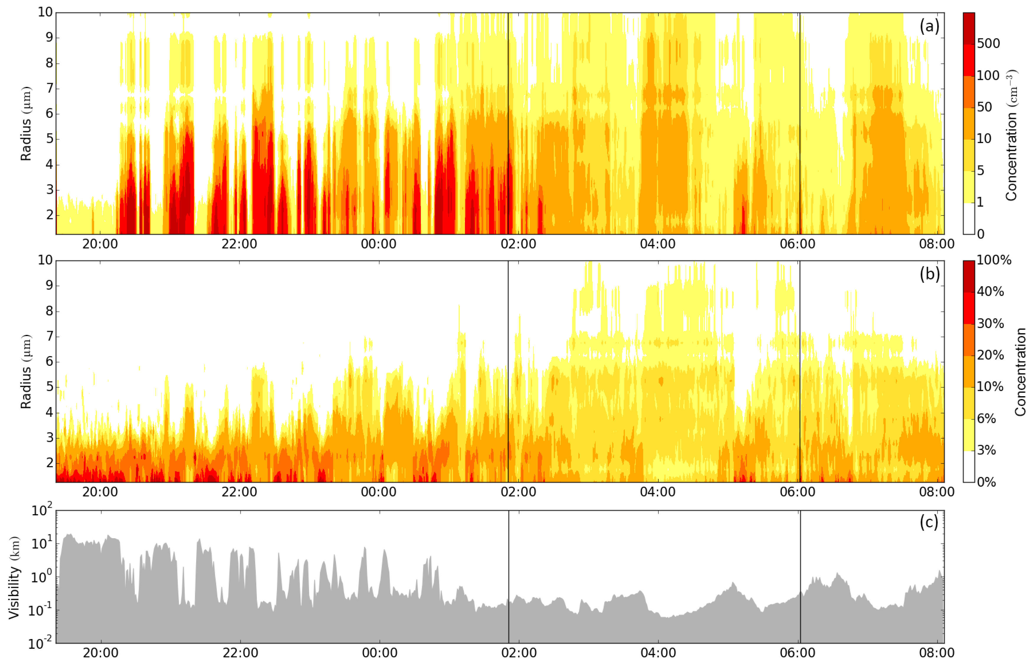
Figure 2 shows the most important parameters measured during Fog Event 1, recorded between 26 October 2011 19:21 UTC and 27 October 2011 08:05 UTC. Subplot a shows absolute drop concentrations (number of drops per cm
3 air volume per 0.5 μm radius interval). Subplot b shows relative drop concentrations (percentage of drops per 0.5 μm radius interval). The ordinate in Subplots a and b, representing the drop radii, only reaches 10 μm because the vast majority of drops had a measured radius between 1 μm and 10 μm. Intervals in which the drop concentration is higher are marked red, whereas intervals with low drop counts are colored white.
During the formation stage, the largest average drop counts of up to were measured, while the mode radius largely remained below 3 μm. However, drop counts showed great temporal variability, as can be seen when looking at the vertical stripe pattern of the absolute drop spectra in this stage. During the mature stage, drop counts decreased to an average of , and the temporal variation in the drop spectra decreased compared to the formation stage. In this stage, mode radii were slightly larger than during fog formation, and a second, smaller local maximum appears at 7 μm in many spectra. This could possibly be the result of an instrument issue, as the maxima around 7 μm are very consistent over all measurements. As these maxima are comparatively small and the MGD has a unimodal shape with maxima usually found around 2 μm to 3 μm, these maxima are flattened out in the fitting procedure of the MGD and thus do not significantly interfere with the results.
Drop counts, mode radii and temporal variation during fog dissipation remained comparable to the values of the mature stage. During fog formation, horizontal visibility was highly variable between and with a general downward trend that reached close to zero by the end of the first stage. Visibility maintained approximately the same level in the mature stage, whereas during dissipation, it rose again, reaching 1.60 km at the end of the event.
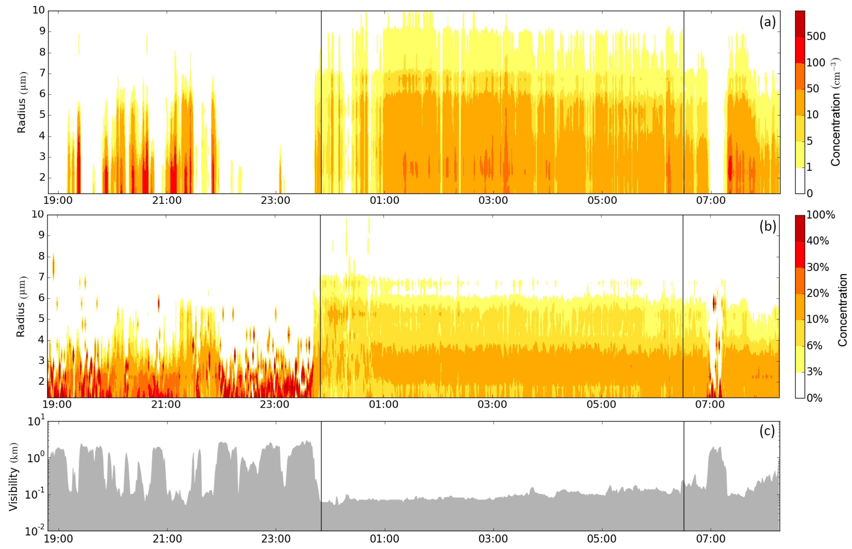
Figure 3 shows the same information for Fog Event 2 recorded between 31 October 2011 17:38 UTC and 1 November 2011 07:55 UTC. This formation stage was also characterized by relatively large drop counts and small mode radii, which never exceeded 3 μm. During the first third of mature fog, large drop counts and small mode radii persisted; in the second third, the drop counts were significantly lower while mode radii rose to 6.75 μm. Towards the end of the mature stage and in the beginning of dissipation, drop counts increased again, while mode radii decreased to values below 2.5 μm. Subplot b reveals a local maximum at 7 μm, similar to the mature stage during the first fog event. After the last drop count maximum in the beginning of the dissipation period, values remained very low and never exceeded
. Visibility values varied between 3.08 km and
during formation, never exceeded 1.00 km during mature fog and, after some hesitation, rose to values between 2.00 km and 4.00 km during dissipation. At the very end of the fog event, it decreased again to
.
The collected data from Fog Event 3, recorded between 13 November 2011 18:48 UTC and 14 November 2011 08:15 UTC are depicted in
Figure 4. The first two thirds of the formation stage were characterized by large drop counts in combination with small mode radii. After that, very few drops were measured over a long period until the beginning of the mature stage when drop radii and counts increased rapidly. Throughout the whole mature stage, drop size spectra with large mode radii up to 7 μm were recorded. This stage was marked by very little variation in both drop counts and mode radii. Besides an abrupt decline around 07:00 UTC, during dissipation, drop radii and counts remained on a relatively even level. Visibility values during fog formation varied between
and 2.95 km with no obvious trend. At the beginning of the mature stage, values decreased very abruptly to below
and remained at this level throughout the entire mature stage. During dissipation, visibility values climbed up to 1.98 km for a short time, fell below
again and then slowly rose to reach values of about
.
In summary, maximal total drop counts appeared during the formation stage of each fog event investigated. The maximal values then continuously decreased through the mature and into the dissipation stages. The same pattern can be seen in the behavior of the mode radius drop counts (
). The highest maximal values of
were recorded during formation and continuously decreased until dissipation. During all three events, mode radii reached the highest recorded values during mature fog and the lowest values during dissipation. Maximal visibility values were observed in the formation stage of each event, but never exceeded 1.00 km during mature fog. During dissipation, a general uptick in visibility, albeit with high variability, could be detected. A brief overview of the information gathered during the three fog events is presented in
Tables S1 and S2 (Supplementary Material), which summarize minimal and maximal values of the most important variables recorded.
3.2. Representativity of Average DSDs for Different Fog Life Cycle Stages
Average spectra were derived separately for each stage of each recorded fog event, as well as for the three combined life cycle stages of all fog events. In addition to the average spectra of the absolute values, the equivalent spectra of the relative values were calculated.
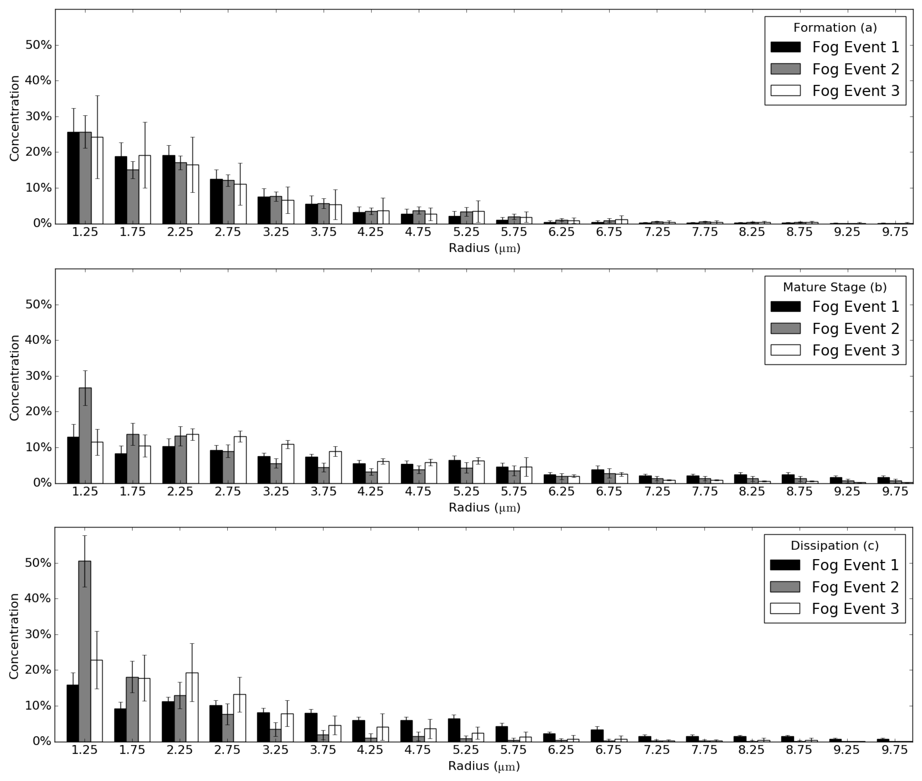
Figure 5 and
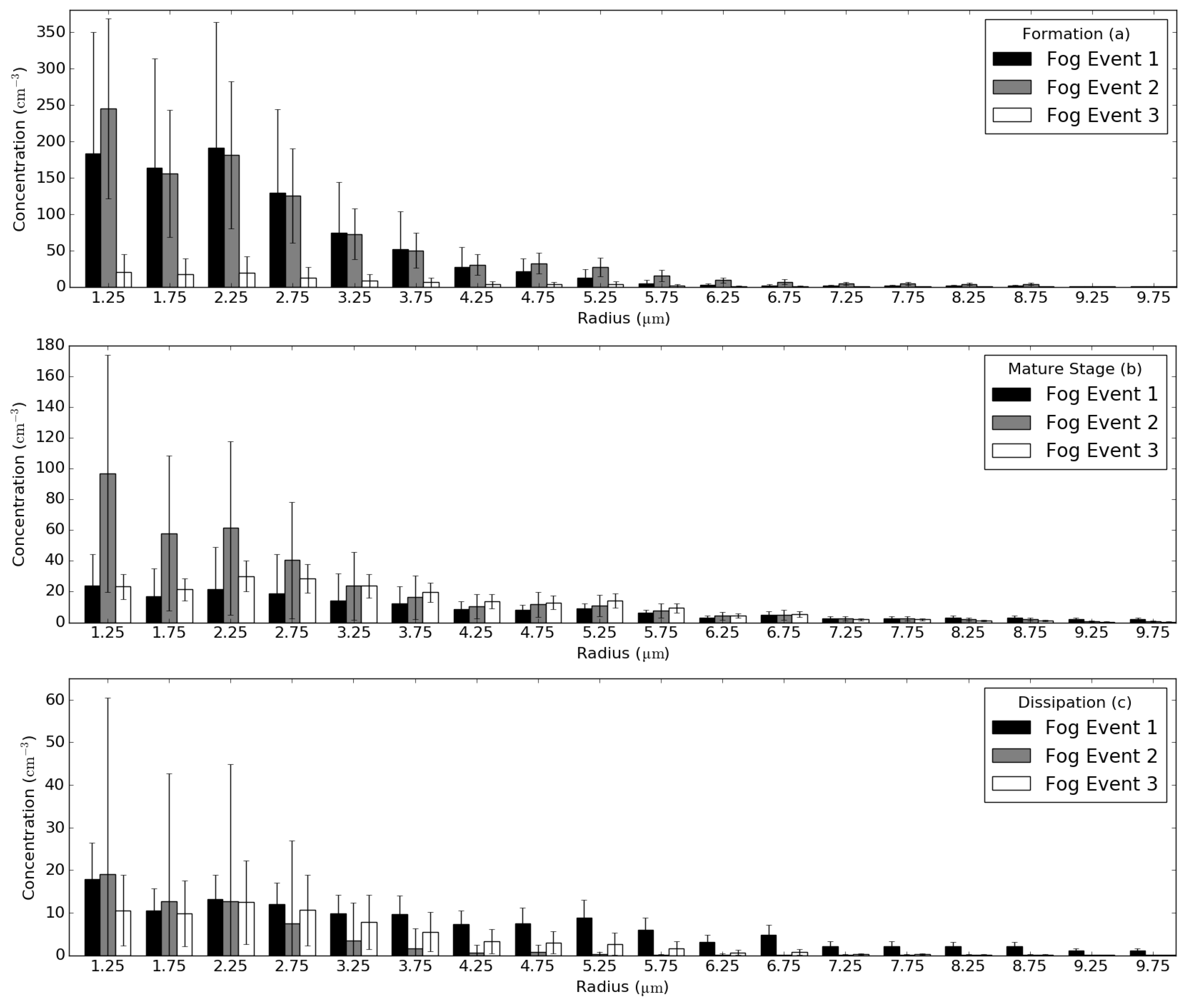
Figure 6 depict the absolute and relative average spectra separately for each stage. Although drop radii ranging from 1 μm to 25 μm were measured, only the first 19 intervals are shown as very few drops above 10 μm were recorded. The bar plots show the formation, mature fog and dissipation stage. Bars indicate stage-averaged values, while error bars denote the standard deviation. Note that the y-axis scale of
Figure 5 is not uniform: absolute drop count averages were generally highest in the formation and lowest in the dissipation stage. All spectra show a slight bimodal structure with local maxima at 1.25 μm and 2.25 μm, although the second maximum is less pronounced than the first one. After the second maximum, the count generally decreases as the radius increases. The standard deviation is highest for small drop radii, where average count values are also highest. During Fog Event 1, most drops were recorded between 1.25 μm and 2.25 μm with a steep decline towards higher radii in the formation stage. In mature fog and during the dissipation stage, small droplets are less present, and the curve takes a more balanced shape. The spectra from the second fog event showed a similar behavior during formation, remained on a relatively high level for small radii in the mature stage, but then rapidly fell to smaller values, although drops with small radii between 1.25 μm and 2.75 μm were generally most frequent. The third fog event showed very similar average spectra in all stages, although drop counts were relatively small as compared to the other two fog events. Here too, small drop radii were best represented. However, during mature fog, the absolute maximum lay at 2.25 μm and drops with higher radii were significantly more common during this stage.
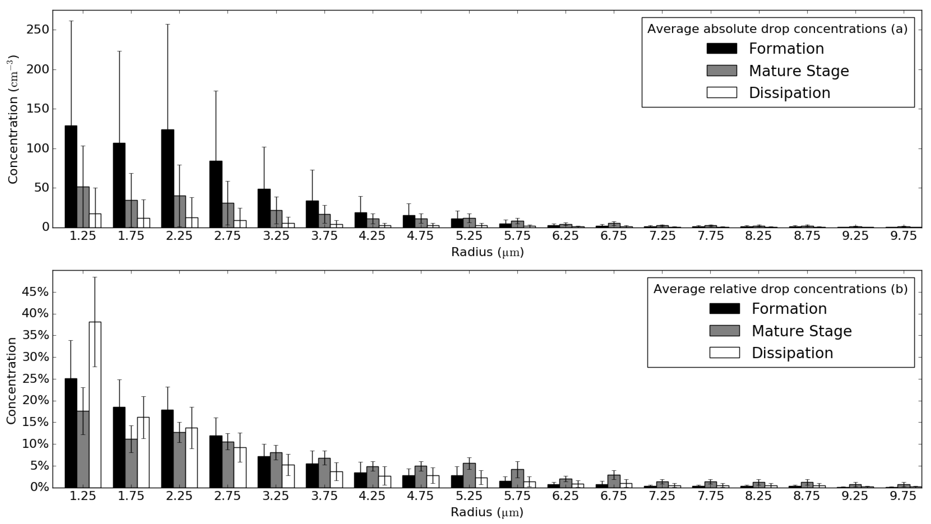
Figure 7 presents absolute and relative average spectra aggregated across all of the fog events in the study. Here, average spectra of all three fog life cycle stages are plotted on one chart. In most cases, absolute drop count averages reached their highest values in the formation stage and lowest in the dissipation stage. Here, considerable variation among small drop radii, the most commonly-occurring drop size, was recorded. All stages showed the previously-mentioned bimodal structure. During the formation stage, average drop counts were higher between radii of 1.25 μm and 2.25 μm although the difference from the other stages became less noticeable with increasing radii. The mature stage was characterized by lower drop counts for smaller radii and relatively high counts for larger radii, surpassing values of the formation stage from 5.25 μm upwards. This gives the average spectrum of the mature stage a more balanced form. Average drop counts during dissipation were generally very small compared to the other stages, and the absolute values showed a flat decline.
Noteworthy is that the values of the relative average spectra were highest during dissipation, which steadily declined as radii increased. Here, the formation and dissipation stage spectra were unimodal (maximum at 1.25 μm). Only the mature stage spectrum continued to show the previously-mentioned bimodal structure, and the relative drop counts were comparably low at smaller radii and high at larger radii, exceeding the values of formation and dissipation at 3.25 μm and upwards. The representativity index of Equation (
A2) was used to evaluate the explanatory power of the stage-averaged spectra.
Table 2 depicts the results: the values represent the mean deviation of all spectra of one stage from the average spectrum of the respective stage, e.g., in the formation stage of Fog Event 1, the recorded spectra deviated from the mean spectrum by
(absolute value) and by 46% (relative value). The absolute spectra always showed highest deviations during the formation and the lowest in the dissipation stage. Overall, formation deviated most from the mean during Fog Event 1 with
, while Fog Event 2 showed the highest deviations in the mature and dissipation stages (
and
, respectively). For all three stages, Fog Event 3 displayed the smallest values for stage-internal deviations from the absolute spectra. Deviations from the relative spectra are marked by different characteristics. Here, maximal deviations were observed during formation and dissipation in Fog Event 3 (79% and 65%, respectively). Compared to Fog Event 3 (19%), the mature stage showed higher values in Fog Events 1 (34%) and 2 (43%). Within the relative spectra, there was no identifiable general trend in the fog life cycle stages. Although Fog Event 1 still reflected the pattern: formation > mature fog > dissipation, this was reversed in Fog Event 2, where the highest deviation values were reached in dissipation (43%) and the lowest values in formation (30%). Fog Event 3 showed yet another behavior with minimal values during mature fog (19%) and far higher values in formation and dissipation (79% and 65%, respectively). The last line in
Table 2 lists deviation values of all spectra of one stage from the respective average spectrum aggregated across all investigated fog events (cf.
Figure 7). Similar to the absolute data of the single fog events, the overall deviations were highest for the formation stage (
) and lowest for the dissipation stage (
). The relative spectra showed the highest deviations for the dissipation stage (60%) and the lowest for mature fog (41%).
3.3. The Z-LWC Relationship
3.3.1. Derived Parameters of the Modified Gamma Distribution
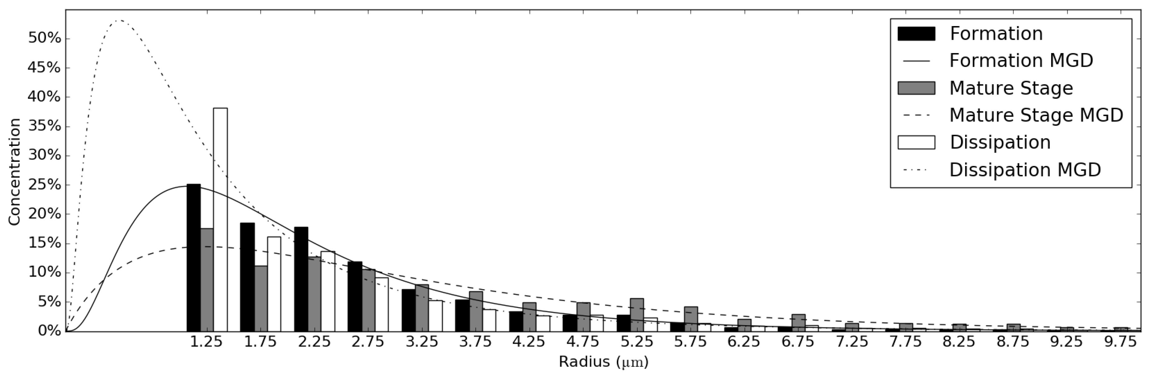
Parameters of the modified gamma distribution (MGD) were derived for each minute-averaged spectrum, as well as for the three stage-averaged spectra. The MGD parameters of the stage-averaged spectra and the respective graphs of the functions over all fog events are presented in
Table 3 and
Figure 8.
values were similar in formation and mature fog, but differed considerably from the dissipation stage (0.50 μm). The Kolmogorov–Smirnov test was applied to each measured 1 min spectrum and its corresponding MGD fit. The acceptance rate at the
significance level was 87.1%, 91.8% and 97.8% for formation, mature stage and dissipation. The good performance of the fits can partly be attributed to the fact that many DSDs showed small total droplet numbers
, which naturally results in larger
p values.
3.3.2. The Proportionality Factor Ω
As a last step, Ω values were derived from each MGD parameter set presented in the previous section. Large Ω values mean that LWG values are large in comparison to the corresponding
Z values (cf. Equation (
A18)). This ratio arises, when the DSD is strongly right-skewed, meaning there are many small droplets and very few large droplets. On the other hand, small Ω values mean that LWG values are small in comparison to the corresponding
Z values, which is the result of a more balanced DSD with fewer small droplets and more large droplets.
Table 4 gives an overview of the most important descriptive measures of Ω in the different fog events (Nos. 1, 2 and 3) and life cycle stages: formation (F), mature stage (M) and dissipation (D). The smallest range, standard deviation and maximum values of Ω were detected in the dissipation stage of Fog Event 1, whereas the largest range and largest maximum values were found in the formation stage of Fog Event 2. Combined over all investigated fog events, the formation stage showed the highest range and the highest maximum with
. The mature stage showed minimal values in range and standard deviation with
and
, respectively. However, these trends are not evident when the single fog events are viewed separately. While the range and standard deviation values decreased throughout the life cycle of Fog Event 1, Fog Event 2 showed the opposite behavior with minimal values in formation and maximum values in dissipation.
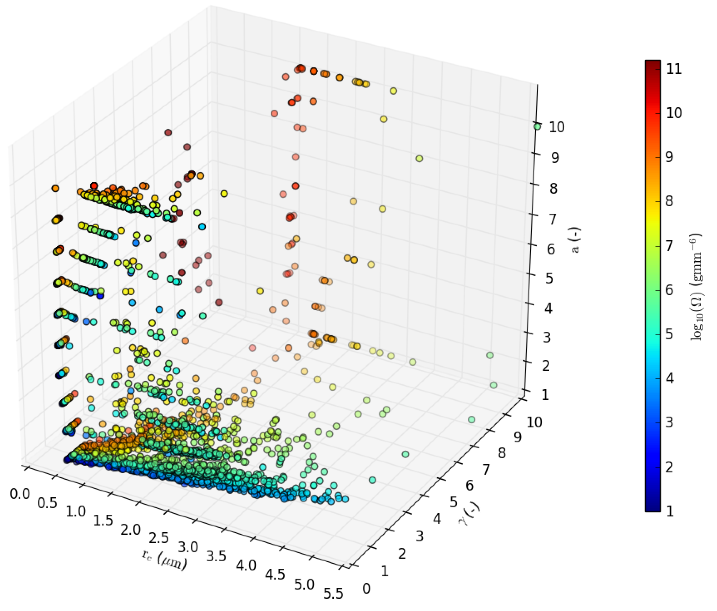
Figure 9 provides an overview of the MGD parameters
,
and
while considering the Z-LWC relationship factor Ω. Each parameter set is colored according to its corresponding Ω value. Ninety percent of the values lay between
and
. Minimal Ω values were only found where all parameters simultaneously had small values. A strip cluster of “blue” sets along the
-axis indicates Ω values that lie below
.
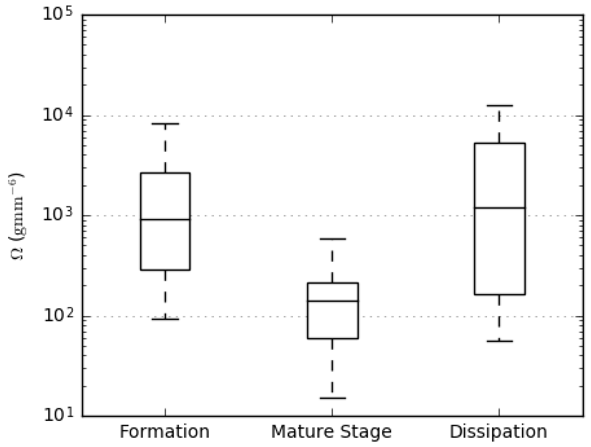
Figure 10 shows the general tendencies of the different Ω distributions. Median Ω values of
in formation,
in mature fog and
in dissipation indicate differences between all three stages.
To test for statistically-significant differences between the three distributions, the non-parametric Kruskal–Wallis one-way analysis of variance by ranks [
39] was conducted, as the data were not normally distributed. Outliers of more than three standard deviations were excluded. Of the 98.77% of the data included, the test reported a statistically-significant difference between the fog life cycle stages (
). In order to determine between which of the three fog life cycle stages these statistically-significant differences can be found, three post hoc Mann–Whitney U-tests [
31] were conducted. The Bonferroni method was used to correct the level of significance, which yielded a total of
. The results showed a significant difference between formation and mature fog (
), as well as between mature fog and dissipation (
). However, no significant difference at the corrected significance level was found between the formation and dissipation distributions (
).
3.3.3. Derivation of Reliable Z-LWC Relationships by Means of Stage-Dependent Characteristic DSDs
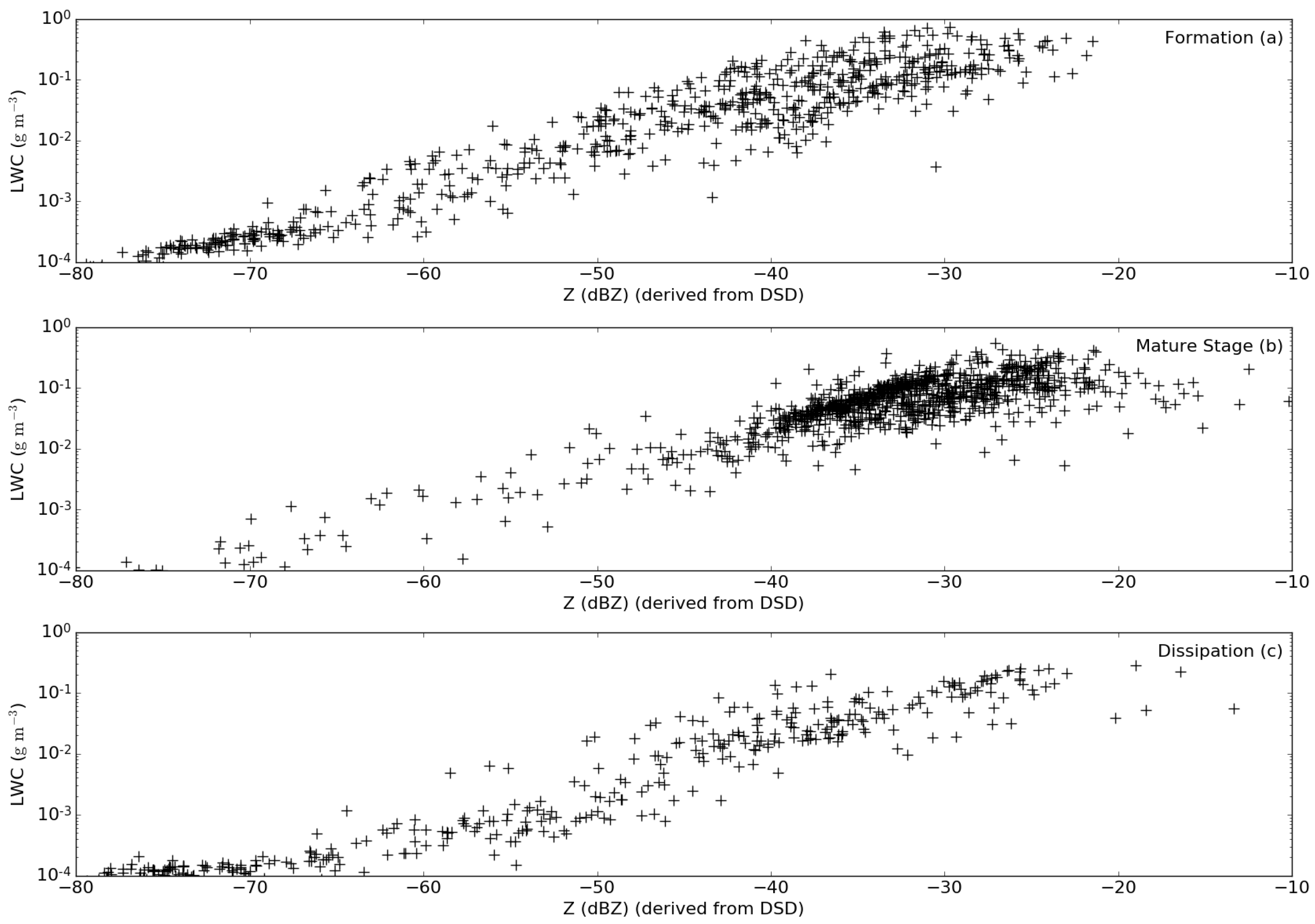
The scatterplots depicted in
Figure 11 show the relationship between Z and LWC for each fog life cycle stage. Both Z and LWC were derived from the MGD parameters using Equations (
A14) and (
A17) in the
Appendix A. The formation stage showed a wide range of Z values with 5% and 95% percentiles at −46.1 dBZ and −28.4 dBZ. No unique LWC value could be assigned to one specific Z value between −45.0 dBZ and −30.0 dBZ, as a vast dispersion of LWC values ranging between
and
occurred. For Z below −60.0 dBZ, the corresponding LWC diminished to marginally small values (
Figure 11a). During mature fog, the range of Z values narrowed considerably, with 90% of the data between −32.7 dBZ and −22.0 dBZ. Nonetheless, the values were generally higher with a mean of −34.3 dBZ compared to −54.1 dBZ in the formation stage. In the mature stage, unique LWC values could be assigned to the respective Z values more precisely, as the dispersion of LWC values was smaller in this stage for constant Z values (
Figure 11b). During the dissipation stage, the range on the Z-axis rose again with 90% of the values between −68.7 dBZ and −27.5 dBZ. The spread of LWC values decreased to a range of
. Due to the narrow range of LWC values for constant Z values, Z values were most accurately assigned to the respective LWC values in the dissipation stage.
The results of the sensitivity tests are listed in
Table 5. The Z values represent values derived from 5% and 95% confidence intervals, as well as median LWC values and the corresponding average spectrum Ω. The minimum of −74.9 dBZ was reached for the formation average spectrum, whereas the maximum was recorded in the mature stage with −25.2 dBZ. LWC values were derived from 5% and 95% confidence intervals, as well as median Z values of the corresponding stage in combination with its average spectrum Ω. The maximum (
) was found in the mature stage, whereas the minimum (
) was found in the dissipation stage.
5. Conclusions
This study investigated the temporal variability of the DSD of fog and its influence on the Z-LWC relationship. In this context, microphysical data of three radiation fog events were analyzed for stage-dependent differences. In addition, fog life cycle stages were tested to determine whether they show typical DSD characteristics, which could be used to separately infer a static relationship between Z and LWC for each stage. As a last step, this information was used to test the feasibility of deriving LWC values directly from radar reflectivity measurements by means of the established relationship factor Ω.
Reliable Z-LWC relationships would enable the retrieval of LWC profiles from cloud radar reflectivity with high temporal and vertical resolution. Besides a better understanding of the microphysical processes involved in fog formation and dissipation, satellite-based fog detection techniques, e.g., Cermak and Bendix [
10], could be improved if reliable LWC profiles were available for initialization and validation. Straightforward fog models, e.g., Reudenbach and Bendix [
47], that rely on columnar LWC data would be able to provide better results if precise LWC input data from radar-based retrievals were available. Finally, these improvements could lead to more precise fog detection and forecasting results.
The results showed that the average DSD of each stage differed from those of the other stages in mode radius, kurtosis and skewness. However, general DSD characteristics for the stages could not be derived because of their inherent heterogenic structure. The variability within each stage combined with the fact that each stage showed different properties dependent on the particular fog event prevented the identification of one specific fog-independent relationship factor for the life cycle stages. To gain more significant results, more continuous DSD measurements during different radiation fog events on the ground, as well as vertical profiles are needed.
Concerning the applied MGD, it has to be mentioned that every fitting approach has its intrinsic limits and errors, which affect the output results. Following former studies related to fog DSD, the MGD is appropriate for reliably representing the various DSDs during the respective development stages of radiation fog events, e.g., Tampieri and Tomasi [
48], Tomasi and Tampieri [
49] and Maier et al. [
4]. However, studies related to DSD of raindrops indicated that even the three-parameter MGD shows limitations comparing the modeled to the measured DSDs, e.g., Joss and Gori [
50], Ulbrich [
51] and Adirosi et al. [
38]. To some extent these limitations can also be stated for the derived MGD parameters in this study. For example, due to the lack of information about droplet counts in the radius range between 0 μm and 1 μm, the derived MGD parameters might be imprecise. With respect to the relationship between Z and LWC, it would be possible to retrieve both parameters from the measured DSDs and to use a nonlinear regression to obtain coefficients relating LWC to Z, instead of using the proportionality factor Ω. One disadvantage in the mentioned approach, however, would be the complete omission of the small droplet sizes below 1 μm radius, which might also lead to inaccuracies in the retrieved Z-LWC relationship. Furthermore, it would be difficult to relate the differing Z-LWC relationship directly to the high temporal DSD dynamics during fog development. By using the derived MGD parameters, the comparison with other studies, e.g., Harris [
40], Tampieri and Tomasi [
48], Tomasi and Tampieri [
49], Maier et al. [
4] and Maier et al. [
30] is facilitated. Nevertheless, the difference between both procedures should be investigated in future studies, using more continuous DSD measurements during different radiation fog events.
The DSD measurements for the fog events observed will be made freely available for download at
www.lcrs.de (data).


