Article

A Matrix-Free Posterior Ensemble Kalman Filter Implementation Based on a Modified Cholesky Decomposition

by
Elias D. Nino-Ruiz
Applied Math and Computational Science Laboratory, Department of Computer Science, Universidad del Norte, Barranquilla 080001, Colombia
Atmosphere 2017, 8(7), 125; https://doi.org/10.3390/atmos8070125
Submission received: 31 March 2017 / Revised: 10 July 2017 / Accepted: 12 July 2017 / Published: 18 July 2017
(This article belongs to the Special Issue Efficient Formulation and Implementation of Data Assimilation Methods)

Abstract

:
In this paper, a matrix-free posterior ensemble Kalman filter implementation based on a modified Cholesky decomposition is proposed. The method works as follows: the precision matrix of the background error distribution is estimated based on a modified Cholesky decomposition. The resulting estimator can be expressed in terms of Cholesky factors which can be updated based on a series of rank-one matrices in order to approximate the precision matrix of the analysis distribution. By using this matrix, the posterior ensemble can be built by either sampling from the posterior distribution or using synthetic observations. Furthermore, the computational effort of the proposed method is linear with regard to the model dimension and the number of observed components from the model domain. Experimental tests are performed making use of the Lorenz-96 model. The results reveal that, the accuracy of the proposed implementation in terms of root-mean-square-error is similar, and in some cases better, to that of a well-known ensemble Kalman filter (EnKF) implementation: the local ensemble transform Kalman filter. In addition, the results are comparable to those obtained by the EnKF with large ensemble sizes.

1. Introduction

Data Assimilation is the process by which imperfect numerical forecasts and sparse observational networks are fused in order to estimate the state x * R n × 1 of a system [1] which (approximately) evolves according to some model operator,
x p * = M t p 1 t p x p 1 * , for 1 p M ,
where, for instance, M : R n × 1 R n × 1 is a numerical model which mimics the ocean and/or the atmosphere dynamics, n is the number of model components, M is the number of observations (which form the assimilation window), and p denotes time index at time t p . Sequential and smoothing methods are commonly utilized in order to perform the estimation process [2,3,4]. In the context of sequential data assimilation, a forecast state x b R n × 1 is adjusted according to a real observation y R m × 1 , where m is the number of observed components from the numerical grid. When Gaussian assumptions are done over background and observational errors, background (forecast) errors can be characterized by,
x N x b , B ,
while observational errors are described by,
y N H x , R ,
where B R n × n is the unknown background error covariance matrix, H : R n × 1 R m × 1 is the observation operator, and R R m × m stands for the data error covariance matrix. By using Bayes rule, the prior (2) and the likelihood (3) distributions can be harnessed in order to estimate the posterior error distribution,
P x | y exp J ( x ) ,
where
J ( x ) = 1 2 · x x b B 1 2 + 1 2 · y H x R 1 2 ,
is well-known as the three dimensional variational cost function. The posterior mode of the distribution (4) can be computed via the minimizer of the cost function (5),
x a = arg min x J ( x ) ,
where x a R n × 1 is well-known as the analysis state. The solution of the optimization problem (6) can be computed as follows,
x a = x b + A · H T · R 1 · y H x b R n × 1 ,
where H ( x ) H T R n × m is a linearized observation operator (with the linearization performed about the background state) and the analysis covariance matrix reads,
A = B 1 + H T · R 1 · H 1 R n × n .
Typically, the moments of the prior distribution can be estimated based on an ensemble of model realizations [5]. However, since ensemble members come at high computational costs owing to current operational data assimilation settings (i.e., numerical grid resolutions), ensemble sizes are bounded by the hundreds while their underlying error distributions range in the order of billions [6]. Consequently, sampling errors can impact the quality of the analysis state [7]. In practice, localization methods can be utilized in order to mitigate the impact of sampling errors during the assimilation steps [8]. For instance, in the EnKF implementation based on a modified Cholesky decomposition (EnKF-MC) [9,10], the covariance matrix estimator proposed by Bickel and Levina in [11] and the conditional independence of model components regarding their spatial distances are exploited in order to estimate a sparse precision matrix of the background distribution, to reduce the computational cost of the analysis step, and to mitigate the impact of spurious correlations during the assimilation of observations. Given the relation between A and B 1 in (7b) and by using the Bickel and Levina estimator, we think that a sparse precision matrix of the analysis distribution can be estimated without the needing of actually computing (7b), and therefore, the assimilation of observations can be efficiently performed.
This paper is organized as follows: in Section 2, efficient implementations of the EnKF which account for localization are discussed, Section 3 presents a matrix-free posterior ensemble Kalman filter implementation based on a modified Cholesky decomposition; in Section 4, experimental tests are performed making use of the Lorenz-96 model in order to assess the accuracy of the proposed method, and finally, Section 5 states the conclusions of this research.

2. Preliminaries

2.1. The Ensemble Kalman Filter

The ensemble Kalman filter (EnKF) is a sequential Monte-Carlo method for parameter and state estimation in highly non-linear models [12]. The popularity of the EnKF owes to his simple formulation and relatively ease implementation [13]. In the EnKF context, an ensemble of model realizations is utilized,
X b = x b [ 1 ] , x b [ 2 ] , , x b [ N ] R n × N ,
in order to estimate the moments of the background error distribution (2) via the empirical moments of the ensemble,
x b x ¯ b = 1 N · e = 1 N x b [ e ] R n × 1 ,
and,
B P b = 1 N 1 · Δ X · Δ X T R n × n ,
where N is the number of ensemble members, x b [ e ] R n × 1 denotes the e-th ensemble member, for 1 e N , x ¯ b is the ensemble mean, P b is the ensemble covariance matrix, and
Δ X = X b x ¯ b · 1 T R n × N ,
is the matrix of member deviations with 1 being a vector of consistent dimension whose components are all ones. When an observation y becomes available, the analysis ensemble can be computed as follows,
X a = X b + P a · Δ Y R n × N ,
where the scaled matrix of innovations on the perturbed observations Δ Y reads,
Δ Y = H T · R 1 · y · 1 T + R 1 / 2 · E H · X b R n × N ,
the columns of matrix E R m × N are samples from a multivariate standard Normal distribution, and
P a = P b 1 + H T · R 1 · H 1 R n × n ,
is the analysis ensemble covariance matrix.

2.2. Localization Methods

As we mentioned before, the ensemble size is much lower than the model resolution ( N n ) and as a consequence, P b is rank-deficient which implies that, the precision matrix (9c) can not be computed. In practice, localization methods are commonly utilized in order to artificially increase the rank of P b and to mitigate the impact of spurious correlations during the analysis steps [14]. In general, we can think in two different flavours of localization: covariance matrix localization [15,16], and spatial localization [17].
In the context of covariance matrix localization, a decorrelation matrix Λ ^ R n × n is typically utilized in order to dissipate spurious correlations between distant model components,
P ^ b = Λ ^ P b R n × n ,
where ∘ denotes component-wise multiplication, P ^ b is a localized covariance matrix, and the components of the localization matrix Λ ^ , for instance, reads,
Λ ^ i , j = exp 1 2 · d i , j 2 r 2 , for 1 i , j n ,
where r is the localization radius, and d i , j stands for the spatial distance between components i and j.
In spatial localization schemes, each model component is surrounded by a local box of radius r and all the information contained within such box is utilized in order to perform a local assimilation step [18]. All local analysis components are then mapped back to the global domain from where a global analysis state is estimated. Some examples of spatial localization are shown in Figure 1 for a two dimensional domain. In general, radius sizes can vary among different model components.
It is important to note that, the use of covariance matrix localization or spatial localization during the assimilation of observations should rely, mainly, on computational aspects [19].

2.3. Efficient EnKF Implementations: Accounting for Localization

An efficient EnKF implementation in the context of spatial localization is the local ensemble transform Kalman filter (LETKF) which belongs to the family of deterministic EnKF formulations [20,21,22,23]. This method has been sucesfully tested in operational data assimilation centres for weather forecast [24]. In the LETKF, the mode of the analysis distribution is estimated in the ensemble space as follows,
x ¯ a = x ¯ b + Δ X · w a R n × 1 ,
where w a = P a ˜ · H · Δ X T · y H x ¯ b R N × 1 , and P a ˜ R N × N is a projection of the analysis covariance matrix (9c) onto such space wherein the ensemble covariance matrix (8c) is well-conditioned. The analysis ensemble is then built about the estimated state (11a) as follows,
X a = x ¯ a · 1 T + N 1 · Δ X · P a ˜ 1 / 2 R n × N .
The assimilation step (11) is applied to each model component for a given radius of influence r from where the global analysis state is obtained. Hence, since the most expensive computation during the assimilation step of LETKF is the inversion of P a ˜ , the computational effort of the LETKF reads,
O φ · n · N 3 ,
where φ denotes the local box sizes.
Another efficient EnKF implementation which makes use of covariance matrix localization is the EnKF based on a modified Cholesky decomposition (EnKF-MC) [25]. In this context, given a radius of influence r, uncorrelated errors are assumed between the component i and the model components P ( i , r ) , for 1 i n , where P ( i , r ) stands for the predecessors of component i whose spatial distances do not exceed r. For a component i, the predecessors P ( i , r ) depend on some ordering of grid components, for instance, Figure 2 shows an example for a two dimensional domain when r = 1 , i = 6 , and grid components are labelled by using column-major format. In the EnKF-MC, the resulting estimator B ^ 1 can be obtained in terms of Cholesky factors by using the Bickel and Levina estimator,
B 1 B ^ 1 = L T · D 1 · L R n × n ,
where L R n × n is a lower triangular matrix,
L i , j = β i , j , j P ( i , r ) 1 , i = j 0 , o t h e r w i s e ,
whose non-zero sub-diagonal elements are obtained by fitting models of the form,
x [ i ] T = j P ( i , r ) β i , j · x [ j ] T + γ i R N × 1 , 1 i n ,
x [ i ] T R N × 1 denotes the i-th row (model component) of the ensemble (8a), and the components of vector γ i R N × 1 are samples from a zero-mean Normal distribution with unknown variance σ 2 . Likewise, D R n × n is a diagonal matrix whose diagonal elements read,
D i , i = var ^ x [ i ] T j P ( i , r ) β i , j · x [ j ] T 1 var γ i 1 = 1 σ 2 > 0 , with D 1 , 1 = var ^ x [ 1 ] T 1 ,
where var ( ) and var ^ ( ) denote the actual and the empirical variances, respectively.
By using the precision matrix (12a), the analysis covariance matrix (7b) can be estimated as follows,
A ^ = B ^ 1 + H T · R 1 · H 1 R n × n .
Thusly, the posterior ensemble is given by,
X a = X b + A ^ · Δ Y R n × N .
Notice, since the number of predecessors for each model component depends on r, the resulting factor (12b) can be sparse, this implies huge savings in terms of memory usage under current operational data assimilation settings wherein n can be very large. Besides, B ^ 1 can be represented in terms of his Cholesky factors and therefore, efficient manners to compute the ensemble (12f) can be derived. Since the number of predecessors is some multiple of the local box sizes, the computational effort of the analysis step in the EnKF-MC can be expressed as follows,
O φ 2 · m · n + φ 2 · n ,
which is linear with regard to n and m. Note that, the EnKF-MC and the LETKF provide similar computational costs.
We think that, by updating the Cholesky factors of (12e) it is possible to obtain an estimate of the precision matrix A 1 in terms of sparse Cholesky factors which can be exploited during the assimilation step (12f) in order to avoid the explicit solution of the linear system,
B ^ 1 + H T · R 1 · H · Z = Δ Y ,
and yet, to derive another efficient implementation of the assimilation cycle. The next section presents an EnKF implementation based on this general idea.

3. A Posterior Ensemble Kalman Filter Based On Modified Cholesky Decomposition

Before we start the derivation of our filter implementation, we assume that, the observational operator is nearly linear and/or it can be easily applied [26], the data error covariance matrix possesses a simple structure and/or it can be easily decomposed [27], and that observational networks are sparse [28].

3.1. General Formulation of the Filter

To be concise, we want to obtain an estimate of the precision matrix for (12e) of the form,
A ^ 1 = B ^ 1 + H T · R 1 · H = L T · D · L + H T · R 1 · H = L ^ T · D ^ · L ^ R n × n ,
where L ^ R n × n is a sparse lower triangular matrix whose diagonal elements are all ones and D ^ R n × n is a diagonal matrix. In this manner, we can approximate the posterior mode of the error distribution,
x ¯ a = x ¯ b + B ^ 1 + H T · R 1 · H 1 · Δ y = x ¯ b + Δ x a ,
via the solution of a lower and an upper triangular system of equations,
L ^ T · D ^ · L ^ · Δ x a = Δ y R n × 1 ,
which can be solved by using forward and backward substitutions, where Δ y = H T · R 1 · y H x ¯ b R n × 1 is the scaled innovation vector on the observations. Note that, by using x ¯ a and A ^ , an estimate of the posterior error distribution can be proposed as follows:
x N x ¯ a , A ^ ,
and therefore, the posterior ensemble (the analysis ensemble members) can be approximated by either
  • drawing samples from the Normal distribution (15),
    X a = x ¯ a · 1 N T + A ^ 1 / 2 · E = x ¯ a · 1 N T + V a ,
    where V a R n × N is given by the solution of an upper triangular system of equations,
    A ^ 1 / 2 · V a = L ^ T · D ^ 1 / 2 · V a = E R n × N ,
    and the columns of E R n × N are samples from a multivariate standard Normal distribution, or
  • using the synthetic data (9b),
    X a = x ¯ b · 1 N T + A ^ · Δ Y = x ¯ b · 1 N T + V ^ a ,
    where V ^ a R n × N is given by the solution of the next linear system of equations,
    L ^ T · D ^ · L ^ · V ^ a = Δ Y .
Note that, the use of x ¯ b instead of x b [ i ] in Equation (17) does not change the statistical moments of the posterior ensemble, consider, for instance, the e-th column x a [ e ] of matrix X a , for 1 e N ,
E x a [ e ] = E x ¯ b + A ^ · Δ y [ e ] = E x ¯ b + E A ^ · Δ y [ e ] = E 1 N · e = 1 N x b [ e ] + E A ^ · Δ y [ e ] = 1 N · e = 1 N E x b [ e ] + E A ^ · Δ y [ e ] = 1 N · e = 1 N x b + E A ^ · Δ y [ e ] = x b + E A ^ · Δ y [ e ] = E x b [ e ] + E A ^ · Δ y [ e ] = E x b [ e ] + A ^ · Δ y [ e ] ,
where Δ y [ e ] R n × 1 is the e-th column of matrix Δ Y .
The approximation (16) is named the posterior ensemble Kalman filter (P-EnKF) since the analysis ensemble is built based on samples from the posterior distribution (15) while the approximation (17) is called the synthetic posterior ensemble Kalman filter (P-EnKF-S) since synthetic data is utilized in order to compute the analysis increments as is commonly done in stochastic EnKF formulations. Details about the computations of L ^ and D ^ are discussed next.

3.2. Computing the Cholesky Factors of the Precision Analysis Covariance

By letting Z = H T · R 1 / 2 R n × m in (13), the precision analysis covariance matrix can be written as follows,
A ^ 1 = B ^ 1 + Z · Z T = L T · D · L + Z · Z T = L T · D · L + j = 1 m · z [ j ] · z [ j ] T ,
where z [ j ] R n × 1 is the j-th column of matrix Z R n × m , for 1 j m . Consider the sequence of matrices,
A ^ ( 0 ) = L ( 0 ) T · D ( 0 ) · L ( 0 ) = L T · D · L = B ^ 1 , A ^ ( 1 ) = A ^ ( 0 ) + z [ 1 ] · z [ 1 ] T = L ( 1 ) T · D ( 1 ) · L ( 1 ) , A ^ ( 2 ) = A ^ ( 1 ) + z [ 2 ] · z [ 2 ] T = L ( 2 ) T · D ( 2 ) · L ( 2 ) , A ^ ( m ) = A ^ ( m 1 ) + z [ m ] · z [ m ] T = L ( m ) T · D ( m ) · L ( m ) = L ^ T · D ^ · L ^ = A ^ 1 ,
where L ( 0 ) R n × n and D ( 0 ) R n × n are the Cholesky factors of B ^ 1 , note that, at any intermediate step j, for 1 j m , we have,
A ^ ( j ) = L ( j 1 ) T · D ( j 1 ) · L ( j 1 ) + z [ j ] · z [ j ] T = L ( j 1 ) T · D ( j 1 ) + p ( j ) · p ( j ) T · L ( j 1 ) ,
where L ( j 1 ) T · p ( j ) = z [ j ] R n × 1 . By computing the Cholesky decomposition of,
D ( j 1 ) + p ( j ) · p ( j ) T = L ˜ ( j 1 ) T · D ( j ) · L ˜ ( j 1 ) ,
from Equation (19), A ^ ( j ) can be written as follows,
A ^ ( j ) = L ˜ ( j 1 ) · L ( j 1 ) T · D ( j ) · L ˜ ( j 1 ) · L ( j 1 ) = L ( j ) T · D ( j ) · L ( j ) ,
where L ( j ) = L ˜ ( j 1 ) · L ( j 1 ) R n × n . In Equation (20), the components of the factors L ˜ ( j 1 ) and D ˜ ( j ) can be easily computed from the elements of D ( j 1 ) and p ( j ) based on the Dolittle’s method for matrix factorization, it is enough to note that,
L ˜ ( j 1 ) T · D ( j ) · L ˜ ( j 1 ) i , k = δ i , k · D ( j 1 ) i , i + p ( j ) i · p ( j ) k ,
from which, the next equations are then obtained,
D ( j ) n , n = p ( j ) n 2 + D ( j 1 ) n , n ,
L ˜ ( j 1 ) i , k = 1 D ( j ) i , i · p ( j ) i · p ( j ) k q P ( i , r ) D ( j ) q , q · L ˜ ( j 1 ) q , i · L ˜ ( j 1 ) q , k ,
and
D ( j ) i , i = p ( j ) i 2 + D ( j 1 ) i , i q P ( i , r ) D ( j ) q , q · L ˜ ( j 1 ) q , i 2 ,
for n 1 i 1 and k P ( i , r ) , where δ i , j is the Kronecker delta function, and the diagonal elements of L ˜ ( j 1 ) are all ones. In Algorithm 1 the updating process for a column z [ j ] is detailed while the computations of factors L ^ and D ^ for A ^ 1 are shown in Algorithm 2. We also report an estimate of the number of multiplications performed at each step of the proposed algorithms. φ denotes the maximum number of predecessors across all model components. Typically, it will be a function of the radius of influence r with φ n . Note that, since the index k is constrained to the predecessors of component i, the structure of L ( j 1 ) is replicated in L ˜ ( j 1 ) and therefore, the structure of L ( j 1 ) is preserved in L ( j ) . Consequently, the sparsity pattern of L ^ equals that of L .
Algorithm 1 Rank-one update for the factors L ( j 1 ) and D ( j 1 ) .
  1:
function Upd_Cholesky_factors( L ( j 1 ) , D ( j 1 ) , z [ j ] )         ▹COST
  2:
    Compute p ( j ) from L ( j 1 ) T · p ( j ) = z [ j ] .             ▹ O φ · n
  3:
    Compute D ( j ) n , n via Equation (21a).               ▹ O 1
  4:
    for i = n 1 1 do         ▹ n 1 times lines 5–9, O φ 2 · n
  5:
        Set L ˜ ( j 1 ) i , i 1 .                       ▹ O 1
  6:
        for k P ( i , r ) do                 ▹ φ times line 7, O φ 2
  7:
           Compute L ˜ ( j 1 ) i , k according to (21b).            ▹ O φ
  8:
        end for
  9:
        Compute D ( j ) i , i via Equation (21c).               ▹ O φ
10:
    end for
11:
    Set L ( j ) L ˜ ( j 1 ) · L ( j 1 ) .                    ▹ O φ 2 · n
12:
    return L ( j ) , D ( j )
13:
end function
Algorithm 2 Computing the factors L ^ and D ^ of A ^ 1 = L ^ T · D ^ · L ^ .
1:
function Compute_analysis_factors( L ( 0 ) , D ( 0 ) , H , R )               ▹COST
2:
    Set Z H T · R 1 / 2 .                           ▹ O m · n
3:
    for j = 1 m do                    ▹m times line 4, O φ 2 · m · n
4:
        Set [ L ( j ) , D ( j ) ] Upd_Cholesky_factors L ( j 1 ) , D ( j 1 ) , z [ j ]       ▹ O φ 2 · n
5:
    end for
6:
    return L ( m ) as L ^ , D ( m ) as D ^ .
7:
end function

3.3. Computational Cost of the Analysis Step

Once the Cholesky factors of the matrix (13) are estimated, the posterior state (14) can be computed and the analysis ensemble (16) can be built. Putting it all together, the assimilation step of the P-EnKF is detailed in Algorithm 3. Based on the Algorithms 1 and 2, it is clear that the computational effort of the P-EnKF is,
O φ 2 · m · n + φ 2 · n ,
which is linear with regard to the number of model components n and the number of observed components from the model domain m. This computational effort obeys, mainly, to the special structure of the Cholesky factors L ( j ) and L ˜ ( j ) , for 1 j m , and how these structures can be exploited in practice in order to reduce the overall computational effort of the analysis step, for instance, the backward substitution in line 2 of Algorithm 1 can be efficiently performed as follows,
p ( j ) n i + 1 = z [ j ] n i + 1 k P ( i , r ) p ( j ) k · L ( j 1 ) i , k , for 1 i n ,
and therefore, the number of multiplications in this computation is bounded by O φ · n while the matrix multiplication in line 11 can be performed as follows,
L ( j ) i , k = q P ( i , r ) P ( k , r ) L ˜ ( j 1 ) i , q · L ( j 1 ) q , k , for 1 i n , and k P ( i , r ) ,
where, evidently, the maximum number of elements in P ( i , r ) P ( k , r ) is bounded by φ and therefore, the total number of multiplications is bounded by O φ 2 · n . Notice, since the matrices L ( j ) and L ˜ ( j ) are sparse and lower triangular, their non-zero bands can be represented by one-dimensional arrays. In this manner, for instance, the computations derived for the elements of L ( j ) and L ˜ ( j ) can be performed on the elements of such vectors. Efficient matrix storage schemes are now proposed by the literature [29,30] as well as scientific computational languages which exploit such structures in order to speed-up matrix computations and to save memory usage [31]. From here, matrix-free implementations of the P-EnKF can be easily derived in order to make it practical under operational data assimilation settings.
Algorithm 3 Assimilation of observations via the posterior ensemble Kalman filter (16).
1:
function Analysis_P-EnKF( X b , L , D , y , H , R )         ▹ Having, B ^ 1 = L T · D · L .
2:
    Set [ L ^ , D ^ ] Compute_analysis_factors L , D , H , R .
3:
    Compute x ¯ a according to Equation (14).
4:
    Compute the posterior ensemble X a based on Equation (16).
5:
    return X a .
6:
end function
Readily, the computational effort of the P-EnKF-S is similar to that of the P-EnKF. We detail the assimilation step of the P-EnKF-S in Algorithm 4.
Algorithm 4 Assimilation of observations via the posterior ensemble Kalman filter (17) .
1:
function Analysis_P-EnKF( X b , L , D , y , H , R )            ▹ Having, B ^ 1 = L T · D · L .
2:
    Set [ L ^ , D ^ ] Compute_analysis_factors L , D , H , R .
3:
    Compute the posterior ensemble X a based on Equation (17).
4:
    return X a .
5:
end function

3.4. Inflation Aspects

While localization methods reduce the impact of spurious correlations, covariance inflation mitigates the impact of under-estimation of sample variances [32,33,34,35]. Typically, ensemble members are inflated prior the forecast step in order to enrich the background error information for the next assimilation cycle and to reduce the odds of ensemble collapsing. For instance, after the assimilation step of EnKF, the ensemble members (9a) are inflated by a factor of ρ > 1 about the analysis mean,
X a , ρ = x ¯ a · 1 T + ρ · Δ X a ,
where Δ X a = X a x ¯ a · 1 T R n × N are the innovations about the analysis mean. Thus, the (co) variances in P a are inflated by a factor of ρ 2 . This idea can be incorporated in the P-EnKF by noting that, the estimated precision analysis covariance matrix can be inflated as follows,
ρ 2 · A ^ 1 ρ 2 · A ^ 1 = L ^ T · 1 ρ 2 · D ^ · L ^ ,
and therefore, the inflation can be performed before the analysis members are drawn from the distribution (15),
X a , ρ = x ¯ a · 1 T + Z ^ ,
where Z ^ R n × N is given by the solution of the sparse upper triangular system of equations,
L ^ T · 1 ρ · D ^ 1 / 2 · Z ^ = E .
Recall that, the columns of matrix E are samples from a multivariate standard Normal distribution. Note that, the use of covariance inflation does not increase the computational effort of the P-EnKF. Similarly, inflation can be applied to the assimilation step in the P-EnKF-S formulation.

3.5. Main Differences Between the EnKF-MC, the P-EnKF, and the P-EnKF-S

In essence, the EnKF-MC, the P-EnKF, and the P-EnKF-S are stochastic filters based on a modified Cholesky decomposition [11]. Nevertheless, the manner how they operate is quite different. Consider again the analysis covariance matrix (13),
A ^ = B ^ 1 + H T · R 1 · H 1 ,
technically speaking, in the context of the EnKF-MC, the posterior ensemble is built by solving the linear system of equations,
A ^ · Z ^ = Δ Y , with Δ Y = H T · R 1 · y · 1 T + R 1 / 2 · E H · X b ,
where the columns of E R n × N follows a standard Normal distribution. Z ^ can be computed by using the iterative Sherman Morrison formula [36] in order to avoid the direct inversion of A ^ while the trivial linear system,
L ^ T · D ^ 1 / 2 · V a = E ,
is the one to solve in order to compute the analysis increments for the background members in the P-EnKF formulation. Likewise, the linear system to solve in the P-EnKF-S case depends on the Cholesky factors and the synthetic data (9b),
L ^ T · D ^ · L ^ · V a ^ = Δ Y ,
whose solution can be obtained by using backward and forward substitutions. Yet another important difference is that, in the P-EnKF, the computation of the posterior mode is similar to that of square root filter formulations,
x ¯ a = x ¯ b + Δ x a , with L ^ T · D ^ · L ^ · Δ x a = H T · R 1 · y H x ¯ b ,
while the analysis mean,
x ¯ a = 1 N · e = 1 N x a [ e ] R n × 1 ,
provides the estimator of x a in the EnKF-MC and the P-EnKF-S methods.

4. Experimental Results

In this section, we tests the proposed EnKF implementations and compare our results with those obtained by the EnKF-MC and the LETKF implementations discussed in Section 2. We make use of the Lorenz-96 model [37] as our surrogate model during the experiments. The Lorenz-96 model is described by the following set of ordinary differential equations [38]:
d x j d t = x 2 x n 1 · x n x 1 + F for j = 1 , x j + 1 x j 2 · x j 1 x j + F for 2 j n 1 , x 1 x n 2 · x n 1 x n + F for j = n ,
where F is external force and n = 40 is the number of model components. Periodic boundary conditions are assumed. When F = 8 units the model exhibits chaotic behavior, which makes it a relevant surrogate problem for atmospheric dynamics [39,40]. A time unit in the Lorenz-96 represents 7 days in the atmosphere. The experimental settings are described below:
  • An initial random solution is integrated over a long time period in order to obtain an initial condition x 2 * R n × 1 dynamically consistent with the model (22).
  • A perturbed background solution x ˜ 2 b is obtained at time t 2 by drawing a sample from the Normal distribution,
    x ˜ 2 b N x 2 * , 0 . 05 2 · I ,
    this solution is then integrated for 10 time units (equivalent to 70 days in the atmosphere) in order to obtain a background solution x 1 b consistent with the numerical model.
  • An initial perturbed ensemble is built about the background state by taking samples from the distribution,
    x ˜ 1 b [ e ^ ] N x 1 b , 0 . 05 2 · I , for 1 e ^ N ^ ,
    and in order to make them consistent with the model dynamics, the ensemble members are propagated for 10 time units, from which the initial ensemble members x 0 b [ e ^ ] R n × 1 are obtained. We create the initial pool X b ^ 0 of N ^ = 10 6 members.
  • The assimilation window consists of M = 25 observations. These are taken every 3.5 days and their error statistics are associated with the Gaussian distribution,
    y k N H k · x k * , 0 . 01 2 · I , for 1 k M .
    where the number of observed components from the model space is m = 30 . The components are randomly chosen at the different assimilation steps. Thus, H k is randomly formed at the different assimilation cycles.
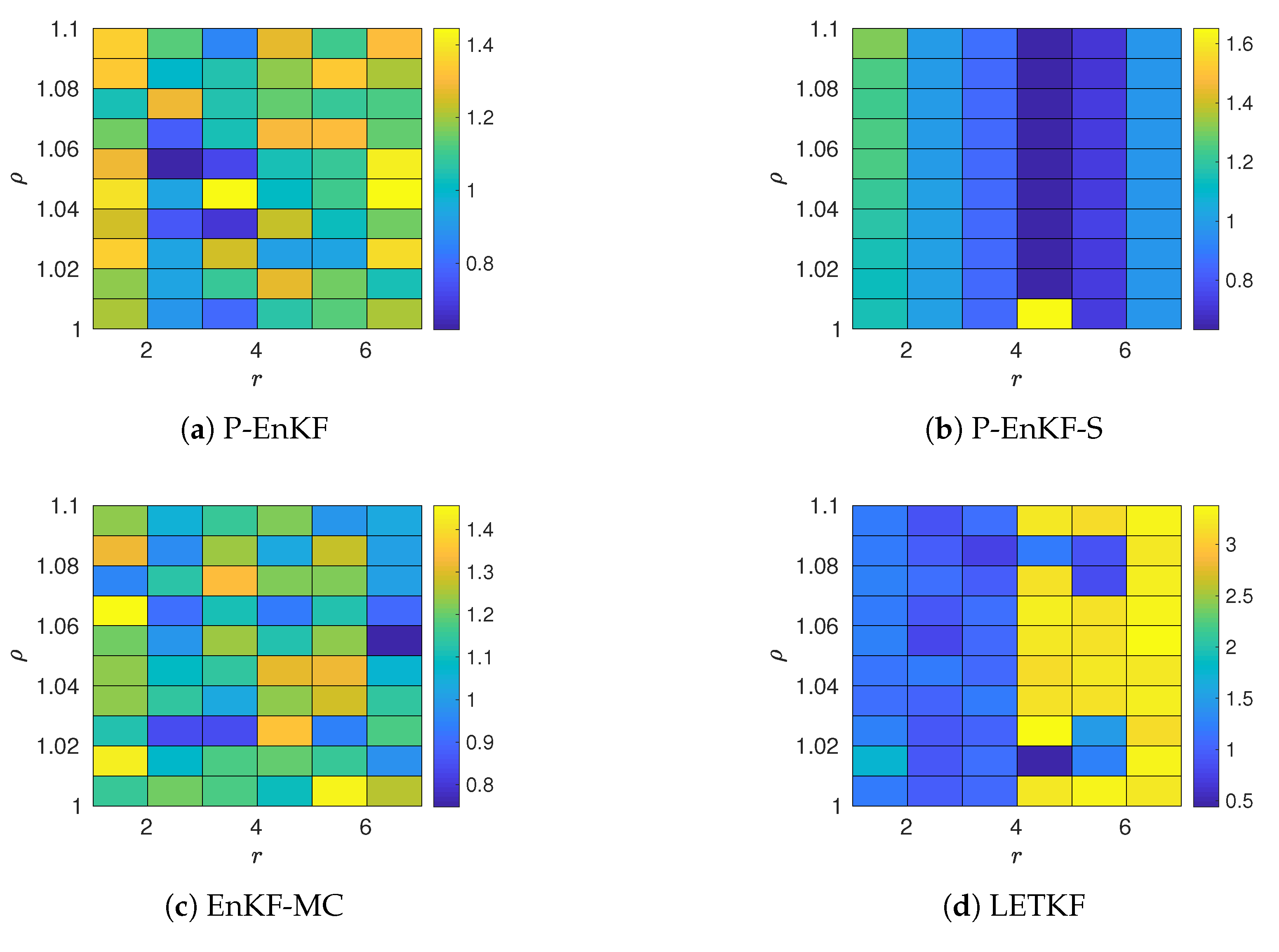
  • Values of the inflation factor ρ are ranged in 1 ρ 1 . 1 .
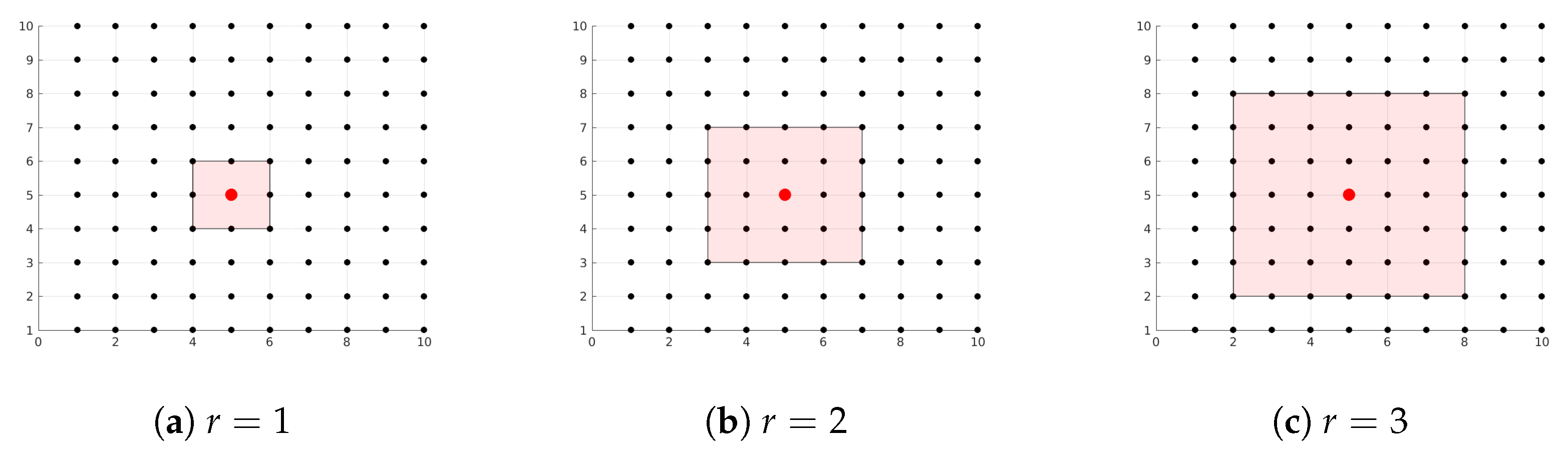
  • We try different values for the radii of influence r, these range in 1 r 7 .
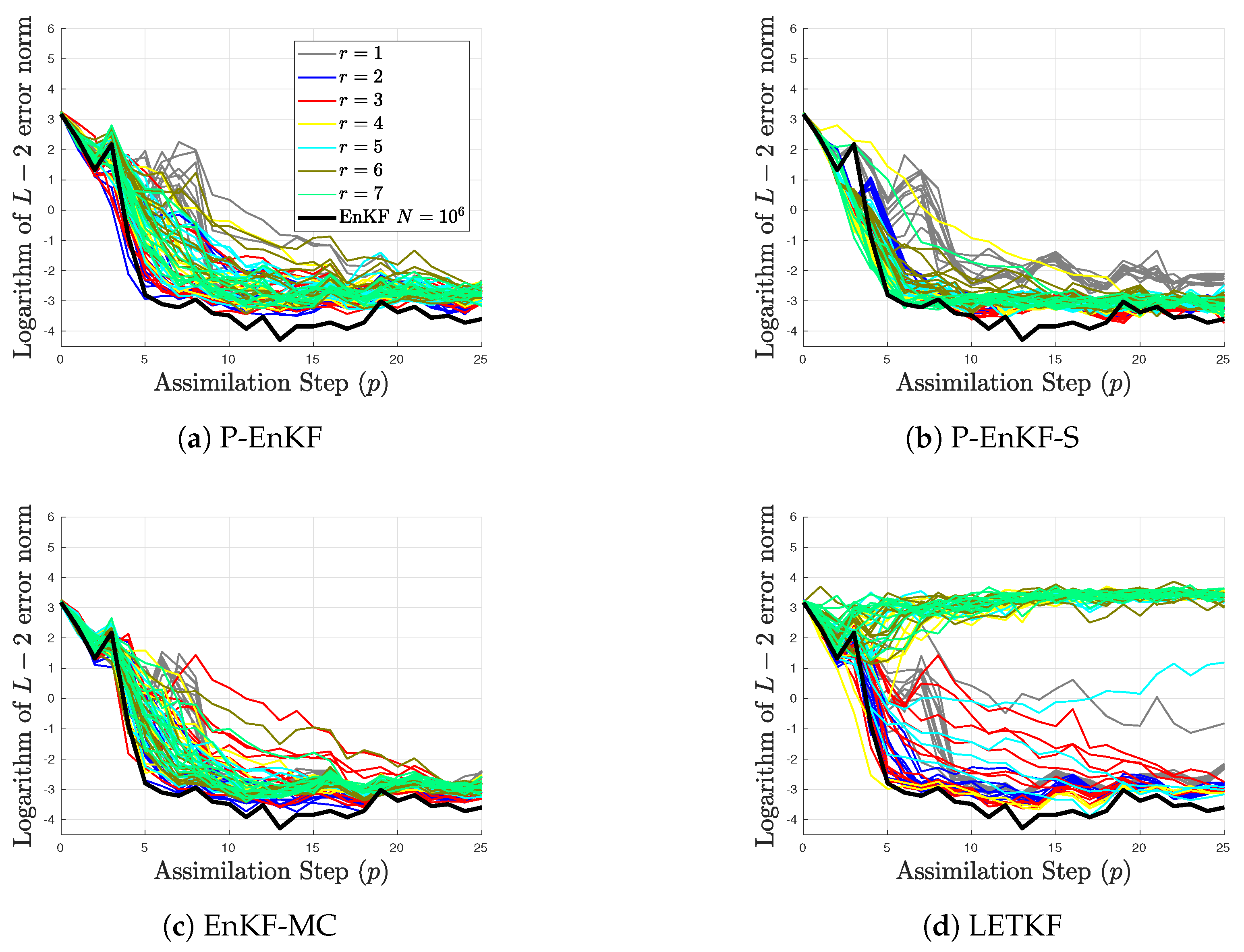
  • The ensemble size for the benchmarks is N = 20 . These members are randomly chosen from the pool X b ^ 0 for the different pairs ( r , ρ ) in order to form the initial ensemble X 0 b for the assimilation window. Evidently, X 0 b X b ^ 0 .
  • The assimilation steps are also performed by the EnKF with full size of X b ^ 0 in order to obtain a reference solution regarding what to expect from the EnKF formulations. Note that, the ensemble size is large enough in order to dissipate the impact of sampling errors. No inflation is needed as well.
  • The L-2 norm of the error is utilized as a measure of accuracy at the assimilation step p,
    λ p = x p * x p a T · x p * x p a ,
    where x p * and x p a are the reference and the analysis solutions, respectively.
  • The Root-Mean-Square-Error (RMSE) is utilized as a measure of performance, in average, on a given assimilation window,
    ϵ = 1 M · p = 1 M λ p 2 .
In Figure 3, the results are shown in terms of L 2 error norms and assimilation steps (p) for the compared methods, we group the results by radius sizes. As can be seen, there are parameter values for r and ρ in which the results proposed by the filters are comparable with those obtained by the EnKF with a large ensemble size of N = 10 6 . This supports the theory that, all filters can provide good approximations of posterior states with just a few ensemble members. However, the performance of the LETKF degrades as the radius size is increased, this can be explained as follows: in the LETKF, local background error correlations are estimated based on a local ensemble covariance matrix, therefore, sampling noise can easily impact the sample covariance matrix when the ensemble size is not much larger than the number of components within the local boxes. Such cases are not evident in the EnKF implementations based on a modified Cholesky decomposition. All these filters perform remarkably well and in all cases, the initial error (uncertainty) is decreased. The importance of having filters which are not so sensible to the parameters r and ρ is that, in practice, such parameters can be hard to tune. Thus, one can prefer filter formulations whose accuracy is not highly impacted by changes in those parameters.
We can analyze the results in terms of RMSE values as well. Those are reported in Figure 4. Note that, as we mentioned before, the accuracy of the LETKF can be sensible to the radius size regardless the inflation factor. After r = 3 , the quality of the analysis obtained by this filter is clearly affected by sampling errors. On the other hand, the proposed filters behave similarly to the EnKF-MC since their background error correlations are estimated making use of the same estimator (12a).

5. Conclusions

This paper proposes a posterior ensemble Kalman filter based on a modified Cholesky decomposition which works as follows: the precision matrix of the background error distribution is estimated in terms of Cholesky factors via a modified Cholesky decomposition, these factors are updated making use of a series of rank-one updates in order to estimate a precision matrix of the posterior distribution. By using this matrix, the posterior mode of the error distribution can be estimated. The posterior ensemble can be built by either sampling from the posterior distribution or making use of synthetic data. Experimental tests are performed in order to assess the accuracy of the proposed method as the inflation factor and the localization radius are varied. The numerical model operator utilized during the experiments is the Lorenz-96 model. The results reveal that the accuracy in terms of root-mean-square-error of the proposed methods are similar to that of the local ensemble transform Kalman filter and even more, our results are comparable to those obtained by the EnKF with large ensemble sizes.

Acknowledgments

This work was supported by the Applied Math and Computer Science Laboratory (AML-CS) at Universidad del Norte, BAQ, COL.

Conflicts of Interest

The author declare no conflict of interest.

References

  1. Lorenc, A.C. Analysis methods for numerical weather prediction. Q. J. R. Meteorol. Soc. 1986, 112, 1177–1194. [Google Scholar] [CrossRef]
  2. Buehner, M.; Houtekamer, P.; Charette, C.; Mitchell, H.L.; He, B. Intercomparison of variational data assimilation and the ensemble Kalman filter for global deterministic NWP. Part I: Description and single-observation experiments. Mon. Weather Rev. 2010, 138, 1550–1566. [Google Scholar] [CrossRef]
  3. Buehner, M.; Houtekamer, P.; Charette, C.; Mitchell, H.L.; He, B. Intercomparison of variational data assimilation and the ensemble Kalman filter for global deterministic NWP. Part II: One-month experiments with real observations. Mon. Weather Rev. 2010, 138, 1567–1586. [Google Scholar] [CrossRef]
  4. Caya, A.; Sun, J.; Snyder, C. A comparison between the 4DVAR and the ensemble Kalman filter techniques for radar data assimilation. Mon. Weather Rev. 2005, 133, 3081–3094. [Google Scholar] [CrossRef]
  5. Nino-Ruiz, E.D.; Sandu, A. Ensemble Kalman filter implementations based on shrinkage covariance matrix estimation. Ocean Dyn. 2015, 65, 1423–1439. [Google Scholar] [CrossRef]
  6. Anderson, J.L. Localization and Sampling Error Correction in Ensemble Kalman Filter Data Assimilation. Mon. Weather Rev. 2012, 140, 2359–2371. [Google Scholar] [CrossRef]
  7. Jonathan, P.; Fuqing, Z.; Weng, Y. The Effects of Sampling Errors on the EnKF Assimilation of Inner-Core Hurricane Observations. Mon. Weather Rev. 2014, 142, 1609–1630. [Google Scholar]
  8. Buehner, M. Ensemble-derived Stationary and Flow-dependent Background-error Covariances: Evaluation in a Quasi-operational NWP Setting. Q. J. R. Meteorol. Soc. 2005, 131, 1013–1043. [Google Scholar] [CrossRef]
  9. Nino-Ruiz, E.D.; Sandu, A.; Deng, X. A parallel ensemble Kalman filter implementation based on modified Cholesky decomposition. In Proceedings of the 6th Workshop on Latest Advances in Scalable Algorithms for Large-Scale Systems, Austin, TX, USA, 15–20 November 2015; p. 4. [Google Scholar]
  10. Nino-Ruiz, E.D.; Sandu, A.; Deng, X. A parallel implementation of the ensemble Kalman filter based on modified Cholesky decomposition. J. Comput. Sci. 2017. [Google Scholar] [CrossRef]
  11. Bickel, P.J.; Levina, E. Regularized estimation of large covariance matrices. Ann. Stat. 2008, 36, 199–227. [Google Scholar] [CrossRef]
  12. Evensen, G. The Ensemble Kalman Filter: Theoretical Formulation and Practical Implementation. Ocean Dyn. 2003, 53, 343–367. [Google Scholar] [CrossRef]
  13. Lorenc, A.C. The potential of the ensemble Kalman filter for NWP—A comparison with 4D-Var. Q. J. R. Meteorol. Soc. 2003, 129, 3183–3203. [Google Scholar] [CrossRef]
  14. Hamill, T.M.; Whitaker, J.S.; Snyder, C. Distance-dependent filtering of background error covariance estimates in an ensemble Kalman filter. Mon. Weather Rev. 2001, 129, 2776–2790. [Google Scholar] [CrossRef]
  15. Cheng, H.; Jardak, M.; Alexe, M.; Sandu, A. A Hybrid Approach to Estimating Error Covariances in Variational Data Assimilation. Tellus A 2010, 62, 288–297. [Google Scholar] [CrossRef]
  16. Chatterjee, A.; Engelen, R.J.; Kawa, S.R.; Sweeney, C.; Michalak, A.M. Background Error Covariance Estimation for Atmospheric CO2 Data Assimilation. J. Geophys. Res. Atmos. 2013, 118. [Google Scholar] [CrossRef]
  17. Keppenne, C.L. Data Assimilation into a Primitive-Equation Model with a Parallel Ensemble Kalman Filter. Mon. Weather Rev. 2000, 128, 1971–1981. [Google Scholar] [CrossRef]
  18. Buehner, M. Evaluation of a Spatial/Spectral Covariance Localization Approach for Atmospheric Data Assimilation. Mon. Weather Rev. 2011, 140, 617–636. [Google Scholar] [CrossRef]
  19. Sakov, P.; Bertino, L. Relation between two common localisation methods for the EnKF. Comput. Geosci. 2011, 15, 225–237. [Google Scholar] [CrossRef]
  20. Tippett, M.K.; Anderson, J.L.; Bishop, C.H.; Hamill, T.M.; Whitaker, J.S. Ensemble Square Root Filters. Mon. Weather Rev. 2003, 131, 1485–1490. [Google Scholar] [CrossRef]
  21. Bishop, C.H.; Toth, Z. Ensemble Transformation and Adaptive Observations. J. Atmos. Sci. 1999, 56, 1748–1765. [Google Scholar] [CrossRef]
  22. Ott, E.; Hunt, B.R.; Szunyogh, I.; Zimin, A.V.; Kostelich, E.J.; Corazza, M.; Kalnay, E.; Patil, D.J.; Yorke, J.A. A local ensemble Kalman filter for atmospheric data assimilation. Tellus A 2004, 56, 415–428. [Google Scholar] [CrossRef]
  23. Hunt, B.R.; Kostelich, E.J.; Szunyogh, I. Efficient data assimilation for spatiotemporal chaos: A local ensemble transform Kalman filter. Phys. D: Nonlinear Phenom. 2007, 230, 112–126. [Google Scholar] [CrossRef]
  24. Ott, E.; Hunt, B.; Szunyogh, I.; Zimin, A.V.; Kostelich, E.J.; Corazza, M.; Kalnay, E.; Patil, D.J.; Yorke, J.A. A Local Ensemble Transform Kalman Filter Data Assimilation System for the NCEP Global Model. Tellus A 2008, 60, 113–130. [Google Scholar]
  25. Nino, E.D.; Sandu, A.; Deng, X. An Ensemble Kalman Filter Implementation Based on Modified Cholesky Decomposition for Inverse Covariance Matrix Estimation. arXiv, 2016; arXiv:arXiv:1605.08875. [Google Scholar]
  26. Sakov, P.; Evensen, G.; Bertino, L. Asynchronous data assimilation with the EnKF. Tellus A 2010, 62, 24–29. [Google Scholar] [CrossRef]
  27. Evensen, G. The ensemble Kalman filter for combined state and parameter estimation. IEEE Control Syst. 2009, 29. [Google Scholar] [CrossRef]
  28. Anderson, J.L. An ensemble adjustment Kalman filter for data assimilation. Mon. Weather Rev. 2001, 129, 2884–2903. [Google Scholar] [CrossRef]
  29. Smailbegovic, F.; Gaydadjiev, G.N.; Vassiliadis, S. Sparse matrix storage format. In Proceedings of the 16th Annual Workshop on Circuits, Systems and Signal Processing, Veldhoven, The Netherlands, 17–18 November 2005; pp. 445–448. [Google Scholar]
  30. Langr, D.; Tvrdik, P. Evaluation criteria for sparse matrix storage formats. IEEE Trans. Parallel Distrib. Syst. 2016, 27, 428–440. [Google Scholar] [CrossRef]
  31. Dongarra, J.J.; Demmel, J.W.; Ostrouchov, S. LAPACK: A Linear Algebra Library for High-Performance Computers. In Computational Statistics: Volume 1, Proceedings of the 10th Symposium on Computational Statistics; Springer Science & Business Media: Berlin, Germany, 2013; p. 23. [Google Scholar]
  32. Westgate, P.M. A covariance correction that accounts for correlation estimation to improve finite-sample inference with generalized estimating equations: A study on its applicability with structured correlation matrices. J. Stat. Comput. Simul. 2016, 86, 1891–1900. [Google Scholar] [CrossRef] [PubMed]
  33. Lei, L.; Whitaker, J.S. Evaluating the tradeoffs between ensemble size and ensemble resolution in an ensemble-variational data assimilation system. J. Adv. Model. Earth Syst. 2017. [Google Scholar] [CrossRef]
  34. Lee, Y.; Majda, A.J.; Qi, D. Preventing catastrophic filter divergence using adaptive additive inflation for baroclinic turbulence. Mon. Weather Rev. 2017, 145, 669–682. [Google Scholar] [CrossRef]
  35. Putnam, B.J.; Xue, M.; Jung, Y.; Snook, N.A.; Zhang, G. Ensemble Probabilistic Prediction of a Mesoscale Convective System and Associated Polarimetric Radar Variables using Single-Moment and Double-Moment Microphysics Schemes and EnKF Radar Data Assimilation. Mon. Weather Rev. 2017. [Google Scholar] [CrossRef]
  36. Ruiz, E.D.N.; Sandu, A.; Anderson, J. An efficient implementation of the ensemble Kalman filter based on an iterative Sherman—Morrison formula. Stat. Comput. 2015, 25, 561–577. [Google Scholar] [CrossRef]
  37. Lorenz, E.N. Designing Chaotic Models. J. Atmos. Sci. 2005, 62, 1574–1587. [Google Scholar] [CrossRef]
  38. Fertig, E.J.; Harlim, J.; Hunt, B.R. A comparative study of 4D-VAR and a 4D ensemble Kalman filter: Perfect model simulations with Lorenz-96. Tellus A 2007, 59, 96–100. [Google Scholar] [CrossRef]
  39. Karimi, A.; Paul, M.R. Extensive chaos in the Lorenz-96 model. Chaos: An Interdiscip. J. Nonlinear Sci. 2010, 20, 043105. [Google Scholar] [CrossRef] [PubMed]
  40. Gottwald, G.A.; Melbourne, I. Testing for chaos in deterministic systems with noise. Phys. D: Nonlinear Phenom. 2005, 212, 100–110. [Google Scholar] [CrossRef]
Figure 1. Local domains for different radii of influence r. The red dot is the model component to be assimilated, the red square denotes components within the scope of r, and components outside the region are unused during the local assimilation process.
Atmosphere 08 00125 g001
Figure 2. Local model components (local box) and local predecessors for the model component 6 when r = 1 . Column-major ordering is utilized to label the model components. (a) In blue, local box for the model component 6 when r = 1. (b) In blue, predecessors of the model component 6 for r = 1.
Atmosphere 08 00125 g002
Figure 3. Experimental results with the Lorenz-96 model (22). The results are grouped by values of r. inflation factors are ranged in 1 ρ 1.1 for each group.
Atmosphere 08 00125 g003
Figure 4. Experimental results with the Lorenz-96 model (22). The The Root-Mean-Square-Error (RMSE) values are shown for the compared filter implementations for different values of r and ρ .
Atmosphere 08 00125 g004

