Abstract
Many researchers have failed to utilize back-calculation to estimate traffic emissions effectively or have obtained unclear results. In this study, the back-calculation of traffic-related PM10 emission factors based on roadside concentration measurements was analyzed. Experimental conditions were considered to ensure the success of back-calculation. Roadside measurements were taken in a street canyon in Shanghai, China. Concentrations from a background site were often found to exceed the measured concentrations at the roadside on polluted days as more errors occurred in the background concentrations. On clean days, these impacts were negligible. Thus, only samples collected on clean days were used in back-calculation. The mean value from back-calculation was 0.138 g/km, which was much smaller than the results obtained using official emission models. Emission factors for light-duty vehicles (LDV), medium-duty vehicles (MDV), heavy-duty vehicles (HDV), and motorcycles were approximately 0.121, 0.427, 0.445, and 0.096 g/km, respectively. The fleet-averaged non-exhaust emission factor was approximately 0.121 g/km, indicating that road dust accounted for 87.7% of the roadside concentration increments. According to the dispersion simulation of reserved samples, the concentrations simulated using back-calculated emission factors were in better agreement with the measured data than the concentrations derived using modeled emission factors.
1. Introduction
Road traffic is a major source of PM in urban air [1,2,3]. However, the quantitative evaluation of its contribution to airborne PM concentrations encounters significant challenges, and the contribution of traffic emissions to air pollution has always been different in the literature. Different approaches have been employed to characterize road traffic emissions [1,4,5]. Research that is based on emission models is common in China. According to the estimations by Wang et al. [6] in Beijing, the ratio of PM10 emission factors from road dust (EFd) to the emission factors from vehicle exhaust (EFe) in 2012 ranged from 19.2 to 184.1, depending on the vehicle type. In 2004, road dust emissions in Shanghai occurred at nearly 146.7 times the rate of PM10 from the vehicle’s exhaust according to a PM10 emissions inventory that was compiled in a previous study [7], in which the authors used the Compilation of Air Pollutant Emission Factors (Ap-42) to evaluate road dust emissions. However, the road dust emissions in this study may have been overestimated because the AP-42 data are based on measurements near dusty roads [8]. EFd derived from field measurements in other countries has not been shown to be significantly greater than EFe. Harrison et al. [9] reported that vehicle-induced resuspension provided a source of strength for road dust (represented by PM2.5-10) approximately equal to that of exhaust emissions (represented by PM2.5) at a roadside in London. According to positive matrix factorization outputs, the PM10 EFd to EFe ratios for LDV and HDV in an urban street canyon in Weststrasse, Zürich were 0.1 and 1.7, respectively [10]. In addition, Abu-Allaban et al. [11] reported that the EFd to EFe ratios for PM10 varied from 1.0 to 18.8 for heavy-duty diesel vehicles and varied from 0.7 to 45.8 for light-duty spark ignition vehicles in Reno when estimated using the chemical mass balance. These studies suggest that the measured emission factors on real roads significantly vary from the results estimated by AP-42. In addition to the difference of applied approaches, the differences of ratios between China and other countries also resulted from many other factors such as the climate and road conditions [12,13,14].
Current research has shown that back-calculations based on concentration measurements can be used to assess emission factors or source strength [15,16,17,18]. Primary back-calculation methods include dispersion models [17,19] and receptor models [20,21,22]. The tracer method has been one of the most popular methods used to back-calculate traffic-related emissions [5,10,23,24]. Gas tracers such as NOx, CO2, and SF6 have been commonly used in studies, whereas reference emission factors for these tracers are typically estimated by emission models. As a result, the accuracy of the emission model is critical to the accuracy of the derived PM10 emission factors. Therefore, the use of the tracer method is not recommended if no proper emission model exists for the tracer. This study addressed back-calculations using dispersion models because dispersion models can be easily modified for use in other locations compared with emission models. Several dispersion models are available for mobile sources, including American Meteorological Society/Environmental Protection Agency Regulatory Model (AERMOD), California Puff Model (CALPUFF), Advanced air dispersion model (ADMS) [25]; Highway air pollution model (HIWAY), Third California Line Source Dispersion Model with queuing and hot spot calculations (CAL3QHC) [26,27]; Fourth California Line Source Dispersion Model (CALINE4) [28]; and Operational Street Pollution Model (OSPM) [29].
However, research that employs back-calculations has often failed to estimate emission factors for roadside emissions or has yielded unclear results. For example, Thorpe et al. [5] reported that roadside PM10 concentrations were lower than background concentrations in some cases. Bukowiecki et al. [10] needed to omit many unqualified samples to ensure the accuracy of their results. The PM2.5 emission factors obtained by Ferm et al. [30] contained great uncertainties as a result of the small PM2.5 concentration increments at the roadside. Generally, uncertainties in the back-calculation of emission factors or source strengths come from measurement and modeling errors [31,32,33]. To estimate traffic-related PM10 emission factors, the ideal concentration increments must be obtained. Particles in urban air come from not only road transport, but also many other sources. Concentration increments must be large enough to ensure the accuracy of the back-calculation [17,34]. Therefore, factors such as the location of the background site, traffic volume, and the diffusion conditions must be considered in the design of any experiment. The impact of these factors has been revealed in previous studies, although this has not been deliberately examined. Many researchers have tended to select background sites near their location of interest. For example, the background site in the study performed by Ketzel et al. [35] was established approximately 500 m from the sampling site. Bukowiecki et al. [10] set their background site approximately 600 m from the sampling site and only kept those samples whose roadside NOx increments were greater than 20 μg/m3. Generally, a nearby site is always superior, unless it is excessively biased. For example, Thorpe et al. [5] found that a greater number of negative roadside PM10 increments appeared when a nearby background site was used. Theoretically, concentration increments are sensitive to road structure, traffic volume, and meteorological conditions. Wang et al. [6] measured PM10 concentrations in a street canyon, an open road, and an intersection in Beijing; the PM10 levels in the street canyon were often significantly greater than those along the open road and in the intersection, while the traffic volume in the street canyon was less than half that along the open road. Previous studies have back-calculated traffic-related emission factors for both open roads and street canyons. In measurements carried out by Abu-Allaban et al. [36], the PM10 levels in a street canyon were found to be higher than those on an open road, while the vehicle volume in the street canyon was lower than that on the open road. Bukowiecki et al. [10] carried out measurements on a freeway and in a street canyon. The freeway was an open road with a large traffic volume of approximately 2083 veh/h, whereas the street canyon was a narrow, occlusive road with only 833 veh/h. Ketze et al. [35] and Amato et al. [23] also examined two street canyons, which registered 1083 veh/h and 792 veh/h, respectively. Conducting measurements in a street canyon appears to support the measurement of high concentration increments under a low traffic volume due to the occlusion of the street canyon. Nevertheless, there is still a dearth of knowledge related to the experimental conditions necessary for successful back-calculations.
In 2014, shortly before this study was conducted, the Ministry of Environmental Protection of China (MEP) released two technical guides for compiling emission inventories of air pollutants associated with road transport. Two emission models were provided to estimate the EFd and EFe of PM10. Compared with exhaust emissions, particles from road dust are more difficult to handle in emission modelling for many reasons [37]. Previous studies have shown that particles from non-exhaust emissions are the predominant source of PM at roadside locations [38,39], whereas the value of dust emission factors was extremely variable. For example, Rauterberg-wulff et al. [40] discovered that the Swedish Meteorological and Hydrological Institute model (SMHI) [41] predicted significantly lower emission factors for road dust than the emission factors obtained by the AP-42 method; Gustafsson et al. [37] summarized the studies of resuspension PM emission factors related to roads. The available studies and emission models provide emission factors that vary over several orders of magnitude, from less than 100.0 mg/km to several thousand mg/km for passenger cars, and a maximum of several tens of thousands mg/km for HDV; Nicholson et al. [42] obtained an estimated PM10 value for resuspended material in the UK of 40.0 mg/km for the vehicle fleet composition; and Luhana et al. [43] recorded significantly lower PM10 emission factors for resuspension: 0.8 mg/km for LDV and 14.4 mg/km for HDV in the UK based on measurements in a tunnel. Therefore, these emission models, especially the dust emission model, need to be examined. However, few published papers have employed emission models released by the MEP to calculate the emission factors.
In this study, traffic-related PM10 emission factors were estimated by both emission models and back-calculation based on roadside concentration measurements, and the results of these two methods were examined by a dispersion simulation. The back-calculation of emission factors was investigated to obtain additional information related to the experimental conditions that are necessary to perform successful back-calculations.
2. Methods
The analysis of this study can be divided into three parts. Part 1 is the back-calculation of traffic-related emission factors: (1) The roadside measurements were carried out to obtain data in the back-calculation, including roadside PM10 concentrations, background PM10 concentrations, traffic volumes, and meteorological conditions. The sampling site and the measurements of parameters are introduced in Section 2.1.1; (2) A dispersion model (OSPM) was used to simulate the dispersion of pollutants in the street canyon. The fleet-averaged emission factor (EFf) was estimated by calculating the source strength in OSPM. Details of the OSPM can be found in Section 2.1.2; (3) Emission factors for different vehicles were calculated using a multiple regression analysis (Section 2.1.3); (4) The fleet-averaged non-exhaust emission factor (EFf,ne) was estimated (Section 2.1.4). Part 2 is the estimation of emission factors with emission models provided by MEP. The exhaust and dust emission models will be introduced in Section 2.2.1 and Section 2.2.2, respectively. Part 3 is the validation of emission factors (Section 2.3).
2.1. Back-Calculation
2.1.1. Roadside Measurements
Sampling Site
Roadside measurements were conducted in a regular urban street canyon in Shanghai (Figure 1). The width of the street canyon was approximately 23 m. Buildings approximately 18 m high were evenly distributed along both sides of the site. The road was a secondary trunk road in an educational and commercial district in the northeast region of Shanghai. Road transport was the primary source of local airborne PM10 in this district. Regular daily cleaning of this road included four manual sweeps, three mechanical sweeps, and two high-pressure washings [44]. As a result, the road was very clean during our field measurements. There were two vehicle lanes and two bicycle lanes. Traffic was dominated by passenger cars interspersed with a small number of vans, buses, and motorcycles. While medium and light trucks were allowed, heavy-duty trucks were prohibited from traveling on the road. A national Phase V emission standard for motor vehicles was brought into effect in Shanghai in 2014. There were approximately 3.04 million vehicles in Shanghai by the end of 2014 [45]. Of the total vehicle population in 2014, approximately 0.6%, 7.4%, 18.2%, 69.0%, and 4.8% met the Phase I, Phase II, Phase III, Phase IV, and Phase V emission standards, respectively. The nearest environmental monitoring station (YP) was located on the roof platform of a five-storey building in a residential area, and next to Yangpu Park. There is no industrial emission source around Station YP, but some low-volume roads are located in the area. The data from Station YP were not directly employed as background concentrations because Station YP was approximately 5.2 km from the measurement site. A background site was established approximately 730 m from the measurement site (Figure 1). The background site was set at an atmospheric environmental monitoring supersite on the roof platform of a five-storey building at Fudan University. There is no industrial emission source at the study area, with the exception of transportation.
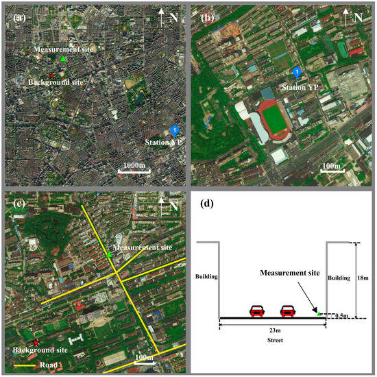
Figure 1.
Measurement and background sites. (a) Locations of measurement site, background site and Station YP; (b) Surroundings of Station YP; (c) Surroundings of measurement site and background site; (d) Measurement site in the street canyon.
Measurements
PM10 mass concentrations were measured with a DustTrakTM dust monitor (Model 8530, Trust Science Innovation, Shoreview, MN, USA) from March to May 2015. The sampling site was located on the pavement near an intersection, as required by the OSPM model. The dust monitor was installed approximately 0.5 m above the ground and 0.5 m from the curb. PM10 concentrations were recorded every minute and averaged every 30 min to reduce the impact of traffic fluctuations on roadside PM10 concentrations. During the roadside concentration measurements, traffic on the street canyon was videotaped by a digital video. The numbers of LDV, MDV, HDV, and motorcycles were also recorded at 30-minute intervals by counting. The LDV included cars and light trucks; the MDV were vans; and the HDV were buses. The average traffic volume was 1135 veh/h, with a maximum volume of 1386 veh/h and a minimum volume of 954 veh/h. The average fleet contained 79.1% LDV, 3.4% MDV, 3.2% HDV, and 14.3% motorcycles. The roadside measurements were conducted during the period of 10:00–12:00 a.m. and 13:00–15:00 p.m. During these periods, the road was accessible and free from congestion according to the videos, so the traffic speeds were relatively stable. The average speed was approximately 25 km/h.
The concentrations at the background site were not measured with the DustTrak concurrently when the roadside concentration measurements were conducted. However, the real-time hourly concentrations at Station YP were recorded during our field measurements. Background concentrations at the background site were corrected from the real-time data at Station YP.
where, (μg/m3) is the background concentration during roadside measurements; (μg/m3) is the real-time data at Station YP during roadside measurements; is the average concentration ratio on individual days; is the real-time data at Station YP before and after roadside measurements; is the concentrations at the background site before and after roadside measurements; and n is the number of records on individual days.
Before and after all the roadside concentration measurements on each sampling day, the DustTrak was moved to the background site for concentration measurements. The concentration data at the background site were collected every minute, and averaged every one hour. Then, these hourly averages were compared with the hourly data released by Station YP in the same period to determine the concentration ratios. Overall, 48 hourly records were obtained (Figure 2) on 13 sampling days. The variations in the hourly concentrations at the background site were relatively consistent with the data at Station YP, with a correlation coefficient of 0.88. The concentration ratios of Station YP and our background site were in the range of 0.82–1.37. The average concentration ratio for the 48 records was 1.08. The average ratios on individual days were also calculated. There were 13 average ratios corresponding to 13 sampling days. These average ratios were in the range of 0.96–1.22. To minimize errors, background concentrations were extrapolated with the average ratios on individual days and real-time data provided by Station YP. Meteorological data from a national monitoring site in Baoshan District were released by the National Meteorological Centre (http://www.nmc.cn/) and were used in the dispersion modeling.
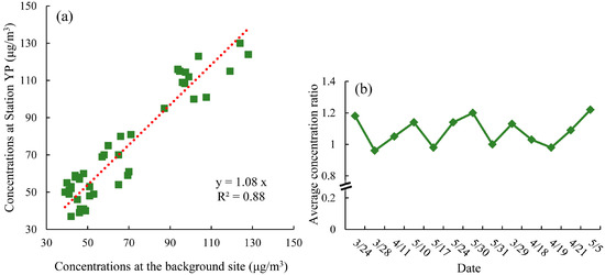
Figure 2.
Comparison of PM10 concentrations at the background site and Station YP (μg/m3). (a) Concentrations at the background site and Station YP; (b) Average concentration ratios on individual days.
A total of 82 samples were obtained of which 27 samples were collected on polluted days (Background concentrations were higher than 90 μg/m3) and 55 were collected on clean days (Background concentrations were lower than 90 μg/m3). The samples were divided into two groups according to the pollution level because some differences exist in the dispersion modeling for stable and unstable atmospheric conditions. Sample details are presented in Section 3.1. The meteorological data and background PM10 concentrations are displayed in Table 1. The average wind speed was approximately 3.4 m/s on clean days and 2.0 m/s on polluted days; the corresponding PM10 background concentrations ranged from 42.3 to 63.5 μg/m3 and 92.7 to 138.4 μg/m3, respectively.

Table 1.
Descriptions of meteorological conditions and background concentrations of PM10 (μg/m3).
2.1.2. The OSPM Model
If the source strength of traffic emission is known, the traffic-related PM10 emission factor can be calculated by Equation (3):
where Q (g/km∙s) is the source strength of traffic emission calculated from the OSPM model and N is the amount of traffic.
A dispersion model (OSPM) can be used to estimate the source strength of traffic emissions. Given the concentrations at the measurement site and the other relevant parameters in the dispersion model, the source strength of traffic emission can be back-calculated. The OSPM model was developed by the Danish National Environmental Research Institute to calculate pollutant concentrations in street canyons [29]. This street canyon model is popular in the literature [5,46,47]. Simplified circulation zone theory was adopted to simulate the turbulence characteristics in the study. The Gaussian diffusion model and a box model were used to simulate the diffusion characteristics of traffic-related pollutants in the street canyon. The concentration of pollutants within the street (Cst) was given by the expression:
where Cd (g/m3) is the direct diffusion concentration; Cr (g/m3) is the recirculation component due to the flow of pollutants around the horizontal vortex generated within the recirculation zone of the canyon; and Cb (g/m3) is the background concentration. The direct concentration was calculated using a Gaussian plume model:
where Q (g/km∙s) is the release rate of emissions in the street; W (m) is the street width; σz is the vertical dispersion parameter at the measurement site; h0 (m) is a constant that accounts for the height of initial pollutant dispersion; and σw (m/s) is the vertical velocity fluctuation due to the mechanical turbulence generated by wind and vehicle traffic in the street. This is described by the relationship:
where u (m/s) is the street-level wind speed; α is a proportionality constant (empirically assigned a value of 0.1); and σw0 (m/s) is the traffic-induced turbulence (empirically assigned a value of 0.1).
The contribution from recirculation was computed using a simple box model and expressed by the relationship:
where Lr (m), Lt (m), Ls1 (m), and Ls2 (m) are dimensions of the recirculation zone; and σwt (m/s) is the ventilation velocity of the canyon expressed as:
where ut (m/s) is the roof-level wind speed; and α and Froof are proportionality constants with values of 0.1 and 0.4, respectively.
2.1.3. Multiple Regression
Multivariate regression was utilized to apportion on-road PM10 to different vehicle classes. When the number of independent variables is k, the model can be described by the following relationship:
where. These variables are independent and identically distributed normal random variables. (g/km) is the value of EFf; (veh/h) is the number of different vehicle types; and (g/km) represents the emission factors for different vehicle classes.
The least square method was applied to calculate the regression coefficients (). If and make the sum of the squared residuals (Equation (8)) a minimum, then and are considered the estimated values of, respectively.
The confidence level for the regression analysis was 0.95 in this study. The intercept was zero because the road was fairly clean, and few emission sources exist, with the exception of transportation.
2.1.4. The Estimation of EFf,ne
The fleet-averaged non-exhaust emission factor was approximated by taking the difference between the EFf obtained by back-calculation and the fleet-averaged emission factor for the vehicle’s exhaust (EFf,e) calculated using the MEP models [48]. The details about the exhaust emission model was displayed in Section 2.2.1.
2.2. Emission Models Recommended by the MEP
PM10 emission factors along the studied road were also estimated using the MEP model. Emission models for wear have not been released by the MEP, so the wear of tires, brakes, and the road surface was not included. The total emission factor was approximated using the sum of the exhaust and road dust:
2.2.1. Exhaust Emission Model
Exhaust emission factors for different vehicle types were calculated using the official emission model [48]:
where (g/km) is the basic emission factor of vehicle i; is the environmental correction factor in area j; is the speed correction factor; is the degradation correction factor; and represents other correction factors, such as the load coefficient and fuel quality. To determine the values of these factors, the proportion of vehicles that met each emission standard was needed. For gasoline vehicles, these values were distributed as follows: 1% Phase I, 10.0% Phase II, 20.0% Phase III, and 69.0% Phase IV. For diesel vehicles, the distribution was 50.0% Phase III and 50.0% Phase IV. LDV and motorcycles were calculated as gasoline vehicles, and MDV and HDV were considered diesel vehicles in this study. For example, according to the documents of EPA [48], when the speed of a vehicle is in the range of 20–30 km/h, the value of is 1.25 for gasoline vehicles; For diesel vehicles, the value of is 1.08 for Phase I to Phase III and 1.12 for Phase IV to Phase V. Therefore, the value of was 1.25 for motorcycles and LDV, and 1.10 for MDV and HDV. The values of these factors are illustrated in Table 2.
Table 2.
Five correction factors of the exhaust emission model.
2.2.2. Dust Emission Model
The emission factor of road dust was determined using the model provided by [49]:
where k (g/km) is the particle size multiplier (0.62 for PM10); SL (g/m2) is the road surface silt loading; W (ton) is the average weight of the vehicles traveling on the road; and is the dust removal efficiency of the pollution control technology. W was estimated according to the following equation:
where (veh/h) is the number of i vehicles; is the proportion of i vehicles; mi (kg) is the average mass of vehicle i; and N is the total number of vehicles. mi values were obtained from the study by [50], and W was set to 1.45 tons in this study. The value of was 55% according to the street cleaning regulations and the dust emission model [44,49].
Road surface silt loading was not measured in this study. The value of SL was taken from the results of [50]. Paved roads in Shanghai were divided into nine types according to traffic volume; SL for the different road types ranged from 0.51 to 4.59 g/m2. The traffic volume for Guoding Road was approximately 1109 PCU/h. According to [50], the value of SL was 3.95 g/m2 when traffic flow ranged from 833 to 1250 PCU/h. This value was used here not only because of the traffic volume, but because the sampling roads in Huang’s study were also located in the central region of the city, and the fleet structures and street cleaning regulations of the sample roads were similar to those of Guoding Road.
2.3. The Validation of Emission Factors
A comparison of the differences between simulated and measured values is a commonly used method to test the results or approach in literatures [6,46]. Several samples were reserved for the validation of emission factors. According to the traffic volumes of these samples and emission factors, the source strengths of emissions from the traffic fleet were estimated with Equation (3). Then, the source strengths of reserved samples were used as the inputs for the OSPM model to simulate the roadside concentrations. By comparing the OSPM modeled concentrations and the measured concentrations, the emission factors were examined. Back-calculated emission factors were also compared with results from other studies in China and other countries to estimate the accuracy of back-calculated emission factors.
3. Results and Discussion
3.1. Roadside Concentration Increments on Clean and Polluted Days
The PM10 concentration increments for different pollution levels are displayed in Figure 3. As shown in Figure 3, the concentration increments on clean days at the sampling site ranged from 7.3 to 24.8 μg/m3 due to local traffic, with a mean concentration increment of approximately 16.5 μg/m3. The concentration increments on polluted days were generally lower than those on clean days, and most of the background concentrations on polluted days were found to be even higher than the concentrations in the street canyon. According to Table 1, the wind direction was variable on both clean and polluted days. However, while negative values appeared under some wind directions on polluted days, they did not appear on clean days under the same wind directions. Therefore, both wind direction was not considered to be the main cause of the occurrence of negative increments. According to the samples collected on polluted days, the wind speeds were 1.5 m/s and 1.7 m/s when large negative increments appeared. The low wind speed and weak turbulence on polluted days may lead to more errors of background concentrations. The concentrations at Station YP were more easily influenced by surrounding sources such as traffic emissions on polluted days because pollutants were hard to diffuse due to the lower wind speed [51,52]. The influence might result in the overestimation of background concentrations indirectly as concentrations at the background site were extrapolated from the data at Station YP. Therefore, there are more errors in the background concentrations on polluted days.
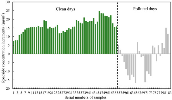
Figure 3.
Roadside concentration increments (μg/m3) on clean days and polluted days.
On polluted days, the estimated background site concentrations were not representative of the background concentrations in the street canyon. Therefore, the samples from polluted days were not utilized in our study. Instead, emission factors were calculated using forty of the samples collected on clean days. The remaining samples were used to validate the obtained emission factors.
The PM10 concentrations on clean days and the corresponding vehicle counts are shown in Figure 4 and Figure 5. ranged from 59.5 to 83.9 μg/m3, while ranged from 42.3 to 63.5 μg/m3. Traffic-related emissions accounted for approximately 24.9% of PM10 concentrations at the sampling site on clean days. The traffic volumes associated with these samples ranged from 954 veh/h to 1386 veh/h. The fleet consisted of an average of 79.1% LDV, 3.4% MDV, 3.2% HDV, and 14.3% motorcycles.
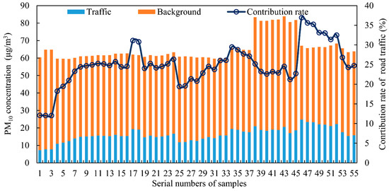
Figure 4.
PM10 concentrations (μg/m3) and contribution rates of traffic to PM10 concentrations (%) in the roadside environment.
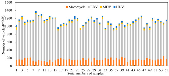
Figure 5.
Number of vehicles per hour (veh/h).
3.2. Emission Factors Calculated Using the MEP Emission Model
Emission factors estimated using the MEP models are listed in Table 3. The results indicated that exhaust-related PM10 was primarily derived from diesel vehicles, especially HDV. As mentioned in Section 2.1.1, buses were the only HDV identified in this study. In the present study, PM10 from one bus was equivalent to PM10 from approximately 45 cars. EFd values for different vehicle classes were not estimated, as the dust emission model was not intended to be used to calculate a separate emission factor for each vehicle weight class. Instead, only one emission factor was calculated to represent the fleet-averaged weight of all vehicles traveling on the road. The average EFf value was 0.017 g/km for the exhaust and 1.423 g/km for road dust. The fleet-averaged emission factor from road dust (EFf,d) was approximately 83.7 times the EFf,e.
Table 3.
Emission factors calculated by emission models (g/km).
3.3. Emission Factors Obtained via Back-Calculation
The EFf values for the 40 samples used in the back-calculation portion of this study varied from 0.085 to 0.183 g/km. The maximum value represented a fleet distribution characterized by 75.8% LDV, 2.9% MDV, 2.9% HDV, and 18.4% motorcycles. The minimum value corresponded to a traffic distribution of 83.0% LDV, 3.6% MDV, 2.1% HDV, and 11.3% motorcycles. The mean EFf was 0.138 g/km. The emission factors for the four vehicle types are shown in Table 4. HDV were associated with the highest emission factor (0.445 g/km), followed by MDV. The HDV and MDV emission factors were over three times greater than the LDV emission factor. Moreover, the standard errors for the HDV and MDV values (0.389 and 0.318 g/km, respectively) were also greater than the LDV value (0.021 g/km). According to the traffic data, LDV occurred at greater rates, and the relative fluctuation of the LDV traffic volume was less than that for HDV and MDV. This may have contributed to the lower standard error for LDV. According to the results of the t-tests, the values of significance for different vehicle classes were smaller than 0.05, which indicated that these results showed statistical significance at the 0.05 significance level. The value of significance for LDV was smallest; it may also be related to the large LDV traffic volume and the low fluctuation of the LDV traffic volume.
Table 4.
Hybrid emission factors for different vehicle classes by multiple regression (g/km).
Based on the modeled EFf,e value, the value of EFf,ne was approximately 0.121 g/km or 7.1 times greater than the EFf,e. Our back-calculation indicated that the contribution of non-exhaust emissions to the overall concentrations was relatively large; however, it was lower than the result obtained using the MEP models
3.4. Comparison of Back-Calculated and Modeled Results
For the reserved 15 samples, the mean concentration increment was approximately 20.1 μg/m3, and the average traffic flow was 1124 veh/h. The average traffic distribution of these 15 samples consisted of 80.0% LDV, 2.7% MDV, 2.8% HDV, and 14.5% motorcycles. The simulated and measured roadside concentrations are both plotted in Figure 6. In Figure 6a, the simulated concentrations ranged from 62.0 to 84.0 μg/m3, and the difference between the measured and simulated concentrations was relatively small. The average relatively difference was 3.6%, with a maximum of 11.6% and a minimum of 0.12%. These values indicated that the simulated concentrations using back-calculated emission factors were consistent with the measured concentrations. Thus, the back-calculated emission factors were considered reliable. In Figure 6b, the corresponding simulated concentrations were in the range of 100.0–290.0 μg/m3, which were much greater than the measured concentrations. The average relatively difference was 156.8%, with a maximum of 245.6% and a minimum of 50.6%, which indicated that the modeled emission factor was substantially overestimated.
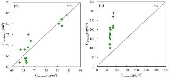
Figure 6.
Comparison of OSPM-simulated and measured roadside concentrations of PM10 (μg/m3). (a) Back-calculated emission factors for different kinds of vehicles were used; (b) Modeled emission factor was used.
The EFf obtained via back-calculation was much lower than that obtained using the emission models. The ratio of the modeled EFf to the back-calculated EFf reached approximately 10.4. The primary difference between the back-calculated results and the modeled results was the non-exhaust emission factor. The modeled EFf,d was approximately 11.8 times that of the back-calculated EFf,ne. Actually, the sampling road was relatively clean due to the regulations of street cleaning, which were even stricter than the regulations in the dust emission model. Therefore, the dust removal efficiency of the pollution control technology () on this road may be higher than the recommended value in the dust emission model. Besides, the average value of SL for secondary trunk roads may overestimate the silt loading level of the Guoding road. These may result in the lower non-exhaust emission factor by back-calculation than that by emission models.
3.5. Comparison with Previous Studies
3.5.1. Fleet-Averaged Emission Factors
Several recent studies have calculated PM10 emission factors based on tunnel tests, roadside tests, or models that provided some basis for comparison with the data presented in this paper. EFf values from recent studies and the value derived in this study are listed in Table 5. Similar results were found in Barcelona, where an emission factor of 0.158 g/km was identified [23]. The EFf value found in the present study was greater than the EFf values found in Los Angeles and Pennsylvania [4,53], Stockholm [54], London [5], Vienna [55], and Zürich and Reiden [10]. This is likely related to the earlier implementation of strict emission standards in Europe and America compared to China. For example, the national Phase V emission standard series came into effect in Shanghai in 2014, while similar standards were adopted six years earlier in the European Union. Nevertheless, the emission factor derived in this study was lower than those identified in Guangzhou and Nanjing [56,57]. The higher percentages of HDV in the Guangzhou and Nanjing fleets (17.6% and 6.3%, respectively) may have contributed to the higher emission factors in these cities. As identified by [58], HDV are a significant source of PM10; therefore, lower HDV numbers relative to the total fleet distribution may result in lower emission levels. The emission factor in the present study was also only a quarter of that estimated for Beijing via AP-42 [6]. The study of [6] was also carried out in spring. Sand storms frequently occurred in Beijing in spring, when road dust may increase significantly due to the sand storms [6]. Although the sand storms formed in the north of China could also influence the PM10 concentrations in Shanghai [59], the influences were much smaller than that in Beijing. Therefore, sand storms may also result in high emission factors in Beijing.
Table 5.
Comparison of the fleet-averaged PM10 emission factor with previous studies (g/km).
3.5.2. Emission Factors for Different Vehicle Types
Emission factors for specific vehicle classes measured in tunnels in other Chinese cities are illustrated in Table 6. Emission levels from the present study were lower than those in Guangzhou, Xiamen, and Nanjing, especially for HDV and motorcycles [56,57,60]. Due to the different regulations of street cleaning in tunnels and on common urban roads, the silt loading in tunnels was generally greater than that on common urban roads, which may be one reason why the PM10 emission factors in tunnel tests are greater than the results found in our study. Differences in speed may also explain the differences in the results. Higher vehicle speeds result in stronger traffic-induced turbulence and wear [61,62]. Studies conducted in other cities also occurred several years earlier than the present study. In the past decade, the Chinese emission standards for vehicle exhausts have become stricter. Vehicle types included in the HDV category may also affect the calculated emission factors for this class. The HDV in the present study were buses; however, other HDV, like heavy trucks, were common in the other studies. For motorcycles, the fuel type affected the emission factor. Motorcycles in the present study were powered by liquefied petroleum gas, while motorcycles in tunnels, e.g., in Xiamen, were powered by gasoline.
Table 6.
Emission factors for different vehicle classes (g/km).
3.6. Uncertainty Analysis of Emission Factors
3.6.1. Uncertainties of Back-Calculation
Dispersion Simulation
The results of back-calculation are dependent on the accuracy of OSPM. The simulation of the concentration with OSPM has inherent uncertainties because OSPM is a simplified empirical model. Previous studies have demonstrated that OSPM is sufficient for the simulation of NO2 in street canyons. Berkowicz et al. [47] compared the measured and modelled concentrations of NO2 at 204 street locations in Copenhagen, and the ratios of the modeled and measured value were 0.88 for monthly concentrations and 0.94 for the average concentrations over six months. Error analyses for the simulation of PM10 using OSPM were limited. However, OSPM has been successfully applied in the simulation of PM10 concentrations in street canyons. For example, Wang et al. [6] compared the OSPM modeled PM10 concentrations in a street canyon with the measured concentrations and found that the modeled concentrations were in close agreement with those of measurements. Additionally, a reasonably good agreement between the measured and OSPM predicted concentrations of PM10 were also observed in the street canyon of Thessaloniki [46].
Measurements
When simulating the dispersion of pollutants in a street canyon, the determination of the meteorological conditions, especially the wind speed and wind direction, plays an important role. For example, concentrations at the leeward side of the street canyon are usually higher than that at the windward side [63]. If the meteorological data is overestimated or underestimated, the dispersion of pollutants would be affected. Then, the estimated emission factor would also be changed. However, meteorological conditions might constantly change, and the variability in meteorological conditions, especially the wind speed and wind direction, would introduce some uncertainties into the results.
No field measurements were performed at the background site at the same time as those in the canyon. Although the background concentrations were corrected from the real-time data at Station YP with average concentration ratios on individual days, uncertainties associated with background concentrations increased, especially on polluted days. The concentrations at Station YP were more easily influenced by surrounding sources on polluted days as the pollutants were hard to diffuse when the wind speeds were low. Therefore, it is important to reduce the influences of surrounding sources on background concentrations. This uncertainty can be mitigated by performing filed measurements at an appropriate background site and performing measurements under favorable weather conditions. Some models such as CFD can be carried out to produce an indication of the potential appropriate background site and favorable weather conditions.
Seasonal Biases
Measurements were performed from March to May in this study. It was spring in China during that period. In some cities of northern China like Beijing, sand storms frequently occurred in spring [6]. Although Shanghai is located at the southeast of China, there were still some influences from sand storms. The PM10 concentrations in spring were much higher than those in summer or autumn [59]. Therefore, the road dust may be higher in spring. Emission factors back-calculated in summer or autumn may be lower than the result in this study.
3.6.2. Uncertainties of Emission Models
Wear Emissions
It’s important to note that the tyre, brake, and road surface wears were not included in this study. Wear is also a very significant source of traffic-related emissions [64,65,66]. USEPA gives an emission factor of 0.005 g/km for tyre wear [67]. In the study of [68], the PM10 emission factors of tyre wear were 0.013 g/km for LDV and 0.200 g/km for HDV; Lükewille et al. [68] indicated that the PM10 emission factors of brake wear were 0.018–0.049 g/km for LDV and 0.035 g/km for HDV; Luhana et al. [43] determined that the LDV and HDV emission factors for road surface wear were 0.003 g/km and 0.029 g/km respectively, although these values were considered highly uncertain. Therefore, the proportion of non-exhaust emission will be greater and the modeled emission factor will be more significantly overestimated if the wear emissions are added.
The Estimation of SL
The value of SL was not measured in this study, although the road type and the traffic volume of the sampling roads in [50] were similar to those in our study. Still, uncertainties would exist in the estimations based on the referenced value. The value 3.95 g/m2 reflected the average level of silt loading on secondary trunk roads in Shanghai, while the value of SL can vary significantly, even on the same type of road [69,70]. It can be seen from the comparison of back-calculated and modeled emission factors, using the average value of SL for a certain type of road, and estimating the dust emission factor may produce some uncertainties. In addition, the value of SL is influenced by not only the road type and traffic volume, but also by many other factors, especially street cleaning. According to the road sweeping records of the Guoding road, the cleaning regulations were strictly met every day. However, the sweeping records of roads in [50] were not available.
The value of SL was changeable, even for the same road, due to the influence of various factors. For example, in 2007, the SL for different types of roads were measured in Beijing [69]. The values of SL were 0.17–1.28 for main road and 0.26–4.43 for the secondary trunk road. In 2014, measurements were performed on the same roads [70]. The values of SL were in the range of 0.17–0.72 g/m2 for the main road and 0.17–1.44 g/m2 for the secondary trunk road. After strengthening the street sweeping, the SL decreased significantly. The values of SL were reduced by 58% and 73% for the main road and the secondary trunk road, respectively. Therefore, the determination of SL in the emission model was highly uncertain.
4. Conclusions
In this study, traffic-related PM10 emission factors for an urban road were back-calculated. The study was performed using data from a street canyon to ensure relatively high concentration increments from local road transportation. Samples collected on clean days were used to successfully back-calculate emission factors. Background concentrations from the background site were not representative of the background concentrations in the street canyon on polluted days. Therefore, the samples collected on polluted days were not utilized in our final back-calculation. Road traffic emission factors were back-calculated using samples from clean days. The mean value of the obtained EFf was 0.138 g/km. The specific emission factors for LDV, MDV, HDV, and motorcycles were approximately 0.121, 0.427, 0.445, and 0.096 g/km, respectively. The EFf,ne value was approximately 0.121 g/km, indicating that road dust was responsible for 87.7% of the concentration increment at the sampling site. The back-calculated emission factors were found to be consistent with observed emission levels on the road, as validated using the reserved samples. The back-calculated emission factors were much smaller than the modeled emission factors. Emission models released by the MEP may have overestimated the road traffic emission levels. Actually, wear emissions were not included in the emission models. The modeled emission factor will be greater if the wear is taken into account.
It is not recommended to measure the PM10 concentrations on polluted days when using the back-calculation method to experimentally determine traffic-related emission factors because there are more errors in the background concentrations on polluted days. The results showed that the success rate of back-calculations could be enhanced by improving the experimental design of a study, particularly by choosing an appropriate background site and optimizing the meteorological conditions under which samples are taken. Some models such as CFD can be carried out to present an indication of the potential appropriate background site and favorable weather conditions before the field measurements are conducted. In addition, the measurements in this study are relatively limited. Therefore, the back-calculation method needs to be tested on more types of streets and roads where the road and climate conditions may be significantly different in the future.
Acknowledgments
This study was supported by the National Natural Science Foundation of China (No. 21107017) and the project of Science and Technology Commission of Shanghai Municipality (No. 15DZ1205303).
Author Contributions
Yuan Wang calculated the data and wrote this paper; Zihan Huang and Yujie Liu conducted the roadside concentration measurements; Qi Yu reviewed the general idea in this paper and the revised paper; and Weichun Ma polished the paper.
Conflicts of Interest
The authors declare no conflict of interest.
Abbreviations
The following abbreviations are used in this manuscript:
| LDV | Light-duty vehicles |
| MDV | Medium-duty vehicles |
| HDV | Heavy-duty vehicles |
| EFd | Emission factor for road dust |
| EFe | Emission factor for vehicle exhaust |
| EFf | Fleet-averaged emission factor |
| EFf,ne | Fleet-averaged non-exhaust emission factor |
| EFf,e | Fleet-averaged exhaust emission factor |
| EFf,d | Fleet-averaged road dust emission factor |
| AERMOD | American Meteorological Society/Environmental Protection Agency Regulatory Model |
| CALPUFF | California Puff model |
| ADMS | Advanced air dispersion model |
| HIWAY | Highway air pollution model |
| CAL3QHC | Third California Line Source Dispersion Model with queuing and hot spot calculations |
| CALINE4 | Fourth California Line Source Dispersion Model |
| OSPM | Operational Street Pollution Model |
| SMHI | Swedish Meteorological and Hydrological Institute Model |
References
- Pant, P.; Harrison, R.M. Estimation of the contribution of road traffic emissions to particulate matter concentrations from field measurements: A review. Atmos. Environ. 2013, 77, 78–97. [Google Scholar] [CrossRef]
- Shen, X.; Yao, Z.; Zhang, Q.; Wagner, D.V.; Huo, H.; Zhang, Y.; Zheng, B.; He, K. Development of database of real-world diesel vehicle emission factors for china. J. Environ. Sci. 2015, 31, 209–220. [Google Scholar] [CrossRef] [PubMed]
- Thomas, K.; Subhasis, B.; Philip, M.F.; Michael, G.; Constantinos, S. Physical and chemical characteristics and volatility of PM in the proximity of a light-duty vehicle freeway. Aerosol. Sci. Technol. 2005, 39, 347–357. [Google Scholar]
- Gillies, J.A.; Gertler, A.W.; Sagebiel, J.C.; Dippel, W.A. On-road particulate matter (PM2.5 and PM10) emissions in the Sepulveda tunnel, Los Angeles, California. Environ. Sci. Technol. 2001, 35, 1054–1063. [Google Scholar] [CrossRef] [PubMed]
- Thorpe, A.J.; Harrison, R.M.; Boulter, P.G.; Mccrae, I.S. Estimation of particle resuspension source strength on a major London road. Atmos. Environ. 2007, 41, 8007–8020. [Google Scholar] [CrossRef]
- Wang, Y.; Li, J.; Cheng, X.; Lu, X.; Sun, D.; Wang, X. Estimation of PM10 in the traffic-related atmosphere for three road types in Beijing and Guangzhou, China. J. Environ. Sci. 2014, 26, 197–204. [Google Scholar] [CrossRef]
- Wu, X.L. The Study of Air Pollution Emission Inventory in Yangtze Delta. Master’s Thesis, Fudan University, Shanghai, China, 30 May 2009. (In Chinese). [Google Scholar]
- CEDA Document Repository. Source Apportionment of Airborne Particulate Matter in the United Kingdom. 1999. Available online: http://cedadocs.ceda.ac.uk/992/ (accessed on 15 January 2017).
- Harrison, R.M.; Yin, J.; Mark, D.; Stedman, J.; Appleby, R.S.; Booker, J.; Moorcroft, S. Studies of the coarse particle (2.5–10 μm) component in UK urban atmospheres. Atmos. Environ. 2001, 35, 3667–3679. [Google Scholar] [CrossRef]
- Bukowiecki, N.; Lienemann, P.; Hill, M.; Furger, M.; Richard, A.; Amato, F.; Prévô, A.S.H. PM10 emission factors for non-exhaust particles generated by road traffic in an urban street canyon and along a freeway in Switzerland. Atmos. Environ. 2010, 44, 2330–2340. [Google Scholar] [CrossRef]
- Abu-Allaban, M.; Gillies, J.A.; Gertler, A.W.; Clayton, R.; Proffitt, D. Tailpipe, resuspended road dust, and brake-wear emission factors from on-road vehicles. Atmos. Environ. 2003, 37, 5283–5293. [Google Scholar] [CrossRef]
- Wang, H.; Chen, C.; Huang, C.; Fu, L. On-road vehicle emission inventory and its uncertainty analysis for Shanghai, China. Sci. Total Environ. 2008, 398, 60–67. [Google Scholar] [CrossRef] [PubMed]
- Han, L.; Zhuang, G.; Cheng, S.; Wang, Y.; Li, J. Characteristics of re-suspended road dust and its impact on the atmospheric environment in Beijing. Atmos. Environ. 2007, 41, 7485–7499. [Google Scholar] [CrossRef]
- Valotto, G.; Rampazzo, G.; Visin, F.; Gonella, F.; Cattaruzza, E.; Glisenti, A.; Formenton, G.; Tieppo, P. Environmental and traffic-related parameters affecting road dust composition: A multi-technique approach applied to Venice area (Italy). Atmos. Environ. 2015, 122, 596–608. [Google Scholar] [CrossRef]
- Chen, Y.H.; Prinn, R.G. Estimation of atmospheric methane emissions between 1996 and 2001 using a three-dimensional global chemical transport model. J. Geophys. Res. 2006, 111, 1984–2012. [Google Scholar] [CrossRef]
- Clarke, K.; Kwon, H.O.; Choi, S.D. Fast and reliable source identification of criteria air pollutants in an industrial city. Atmos. Environ. 2014, 95, 239–248. [Google Scholar] [CrossRef]
- Haupt, S.E.; Young, G.S.; Allen, C.T. A genetic algorithm method to assimilate sensor data for a toxic contaminant release. J. Comput. 2007, 2, 85–93. [Google Scholar] [CrossRef]
- Li, F.; Niu, J. An inverse approach for estimating the initial distribution of volatile organic compounds in dry building material. Atmos. Environ. 2005, 39, 1447–1455. [Google Scholar] [CrossRef]
- Chow, F.K.; Kosovic, B.; Chan, S. Source inversion for contaminant plume dispersion in urban environments using building-resolving simulations. J. Appl. Meteorol. Clim. 2008, 47, 1553–1572. [Google Scholar] [CrossRef]
- Contini, D.; Cesari, D.; Conte, M.; Donateo, A. Application of PMF and CMB receptor models for the evaluation of the contribution of a large coal-fired power plant to PM10 concentrations. Sci. Total Environ. 2016, 560–561, 131–140. [Google Scholar]
- Jaeckels, J.M.; Bae, M.S.; Schauer, J.J. Positive matrix factorization (PMF) analysis of molecular marker measurements to quantify the sources of organic aerosols. Environ. Sci. Technol. 2007, 41, 5763–5769. [Google Scholar] [CrossRef] [PubMed]
- Lan, A.Y.; Jiang, H. Source apportionment of heavy metals in sediment using CMB model. Adv. Mater. Res. 2013, 800, 127–131. [Google Scholar]
- Amato, F.; Nava, S.; Lucarelli, F.; Querol, X.; Alastuey, A.; Baldasano, J.M.; Pandolfi, M. A comprehensive assessment of PM emissions from paved roads: Real-world emission factors and intense street cleaning trials. Sci. Total Environ. 2010, 408, 4309–4318. [Google Scholar] [CrossRef] [PubMed]
- Kam, W.; Liacos, J.W.; Schauer, J.J.; Delfino, R.J.; Sioutas, C. On-road emission factors of PM pollutants for light-duty vehicles (LDVs) based on urban street driving conditions. Atmos. Environ. 2012, 61, 378–386. [Google Scholar] [CrossRef]
- Ministry of Environmental Protection of the People’s Republic of China. Guidelines for Environmental Impact Assessment Atmospheric Environment. 2008. Available online: http://kjs.mep.gov.cn/hjbhbz/bzwb/other/pjjsdz/200901/t20090105_133276.htm (accessed on 15 January 2017). (In Chinese)
- United States Environmental Protection Agency. User’s Guide to CAL3QHC Version 2.0: A Modeling Methodology for Predicting Pollutant Concentrations Near Roadway Intersections. 1992. Available online: http://nepis.epa.gov/Exe/ZyPURL.cgi?Dockey=000033I9.txt (accessed on 15 January 2017).
- United States Environmental Protection Agency. User’s Guide for HIWAY, a Highway Air Pollution Model. 1975. Available online: http://nepis.epa.gov/Exe/ZyPURL.cgi?Dockey=2000X6BE.txt (accessed on 15 January 2017).
- Benson, P.E. Caline4-a Dispersion Model for Predicting Air Pollutant Concentrations Near Roadways; Final report; California Department of Transportation and Federal Highway Administration: Sacramento, CA, USA, 1984.
- Hertel, O.; Berkowicz, R. Operational Street Pollution Model (OSPM); Evaluation of the Model on Data from St. Olavs Street in Oslo. DMU LBFT-Al35; National Environmental Research Institute: Roskilde, Denmark, 1989. [Google Scholar]
- Ferm, M.; Sjöberg, K. Concentrations and emission factors for PM2.5 and PM10 from road traffic in Sweden. Atmos. Environ. 2015, 119, 211–219. [Google Scholar] [CrossRef]
- Gao, Z.; Desjardins, R.L.; Flesch, T.K. Assessment of the uncertainty of using an inverse-dispersion technique to measure methane emissions from animals in a barn and in a small pen. Atmos. Environ. 2010, 44, 3128–3134. [Google Scholar] [CrossRef]
- Lushi, E.; Stockie, J.M. An inverse Gaussian plume approach for estimating atmospheric pollutant emissions from multiple point sources. Atmos. Environ. 2009, 44, 1097–1107. [Google Scholar] [CrossRef]
- Yee, E. Inverse dispersion for an unknown number of sources: Model selection and uncertainty analysis. Isrn. Appl. Math. 2014, 2012, 500–519. [Google Scholar] [CrossRef]
- Zheng, X.; Chen, Z. Inverse calculation approaches for source determination in hazardous chemical releases. J. Loss Prev. Process Ind. 2011, 24, 293–301. [Google Scholar] [CrossRef]
- Ketzel, M.; Wåhlin, P.; Berkowicz, R.; Palmgren, F. Particle and trace gas emission factors under urban driving conditions in Copenhagen based on street and roof-level observations. Atmos. Environ. 2003, 37, 2735–2749. [Google Scholar] [CrossRef]
- Abu-Allaban, M.; Gillies, J.A.; Gertler, A.W. Application of a multi-lag regression approach to determine on-road PM10 and PM2.5 emission rates. Atmos. Environ. 2003, 37, 5157–5164. [Google Scholar] [CrossRef]
- Swedish National Road and Transport Research Institute, Emission of Wear and Resuspension Particles in the Road Environment, 2003. Available online: https://www.vti.se/en/Publications/Publication/emissions-of-wear-and-resuspension-particles-in-th_673864 (accessed on 1 June 2017).
- Forsberg, B.; Hansson, H.C.; Johansson, C.; Areskoug, H.; Persson, K.; Järvholm, B. Comparative health impact assessment of local and regional particulate air pollutants in scandinavia. Ambio J. Hum. Environ. 2005, 34, 11–19. [Google Scholar] [CrossRef]
- Omstedt, G.; Bringfelt, B.; Johansson, C. A model for vehicle-induced non-tailpipe emissions of particles along Swedish roads. Atmos. Environ. 2005, 39, 6088–6097. [Google Scholar] [CrossRef]
- Rauterberg-wulff, E.A. Investigation into the Significance of Dust Resuspension for the PM10 Emission on a Main Road. Report Produced for the Senate Department of Urban Development, Environmental Protection and Technology. Berlin Technical University, 2000. Available online: http://www.dapple.org.uk/Private/DATA/DUST/Berlin%20resuspended%20dust%20report.pdf (accessed on 15 January 2017).
- Johansson, C.; Hadenius, A.; Johansson, P.-Å.; Jonson, T. Shape: The Stockholm Study on Health Effects of Air Pollution and Their Economic Consequences, Part I: NO2 and Particulate Matter in Stockholm, Concentrations and Population Exposure; Vaegverket Publikation: Stockholm, Sweden, 1999. [Google Scholar]
- Department for Environment Food & Rural Affairs. A Review of Emission Factors and Models for Road Vehicle Non-Exhaust Particulate Matter. TRL Report PPR065; 2006. Available online: https://uk-air.defra.gov.uk/assets/documents/reports/cat15/0706061624_Report1__Review_of_Emission_Factors.PDF (accessed on 15 January 2017).
- Luhana, L.; Sokhi, R.; Warner, L.; Mao, H.; Boulter, P.; McCrae, I.S.; Wright, J.; Osborn, D. Measurement of Non-Exhaust Particulate Matter. 5th Framework PARTICULATES project. European Commission Directorate General Transport and Environment, 2004. Available online: http://lat.eng.auth.gr/particulates/deliverables/Particulates_D8.pdf (accessed on 15 January 2017).
- Shanghai Municipal Bureau of Quality and Technical Supervision. Cleaning Quality and Service Requirements for Roads, Public Squares and Accessorial Public Facilities. 2011. Available online: http://www.shzj.gov.cn/art/2011/2/9/art_2828_821.html (accessed on 15 January 2017). (In Chinese)
- Shanghai Statistics Bureau. Shanghai Statistical Yearbook. 2015. Available online: http://www.stats-sh.gov.cn/data/toTjnj.xhtml?y=2015 (accessed on 15 January 2017). (In Chinese)
- Assael, M.J.; Delaki, M.; Kakosimos, K.E. Applying the OSPM model to the calculation of PM10 concentration levels in the historical centre of the city of Thessaloniki. Atmos. Environ. 2008, 42, 65–77. [Google Scholar] [CrossRef]
- Berkowicz, R.; Ketzel, M.; Jensen, S.S.; Hvidberg, M.; Raaschou-Nielsen, O. Evaluation and application of OSPM for traffic pollution assessment for large number of street locations. Environ. Model. Softw. 2008, 23, 296–303. [Google Scholar] [CrossRef]
- Ministry of Environmental Protection of the People’s Republic of China. Technical Guides for Compilation of Air Pollutant Emission Inventory of Road Vehicles (Trial Edition). Beijing, China: Ministry of Environmental Protection of the People’s Republic of China, 2014. Available online: http://www.zhb.gov.cn/gkml/hbb/bgg/201501/W020150107594587831090 (accessed on 15 January 2017). (In Chinese)
- Ministry of Environmental Protection of the People’s Republic of China. Technical Guides for Compilation of Road Dust Emission Inventory (Trial Edition). Beijing, China: Ministry of Environmental Protection of the People's Republic of China, 2014. Available online: http://www.zhb.gov.cn/gkml/hbb/bgg/201501/W020150107594588131490.pdf (accessed on 15 January 2017). (In Chinese)
- Huang, Y.M. Research on Estimation and Distribution Character of Urban Fugitive Dust. Master’s Thesis, East China Normal University, Shanghai, China, 2006. [Google Scholar]
- Zhang, X.W.; Zhu, M.S.; Cao, H.Z.; Wang, H.; Wang, L. Numerical simulation and analysis of pollutant dispersion in the resident district. Low Temp. Archit. Technol. 2008, 1, 121–123. (In Chinese) [Google Scholar]
- Zhuang, S.Q. Study on Mechanism of Gas Flow and Pollutant Dispersion around the Buildings. Master’s Thesis, Northeastern University, Shenyang, China, 2014. [Google Scholar]
- Health Effects Institute. Real-World Particulate Matter and Gaseous Emissions from Motor Vehicles in a Highway Tunnel. 2002. Available online: https://www.healtheffects.org/system/files/GertlerGrosjean.pdf (accessed on 1 June 2017).
- Kristensson, A.; Johansson, C.; Westerholm, R.; Swietlicki, E.; Gidhagen, L.; Wideqvist, U.; Vesely, V. Real-world traffic emission factors of gases and particles measured in a road tunnel in Stockholm, Sweden. Atmos. Environ. 2004, 38, 657–673. [Google Scholar] [CrossRef]
- Handler, M.; Puls, C.; Zbiral, J.; Marr, I.; Puxbaum, H.; Limbeck, A. Size and composition of particulate emissions from motor vehicles in the Kaisermühlen-Tunnel, Vienna. Atmos. Environ. 2008, 42, 2173–2186. [Google Scholar] [CrossRef]
- Wang, B.G.; Zhang, Y.H.; Zhu, C.J.; Yu, K.H.; Chen, L.Y.; Chen, Z.Y. A study on city motor vehicle emission factors by tunnel test. J. Environ. Sci. 2001, 22, 55–59. (In Chinese) [Google Scholar]
- Hu, W.; Qin, Z. A study on PM10 emission factor of motor vehicle by tunnel test in Nanjing city. Chin. J. Environ. Eng. 2009, 3, 1852–1855. (In Chinese) [Google Scholar]
- Li, G.L.; Zhou, M.; Chen, C.H.; Wang, H.L.; Wang, Q.; Lou, S.R.; Qiao, L.P.; Tang, X.B.; Li, L.; Huang, H.Y.; et al. Characteristics of particulate matters and its chemical compositions during the dust episodes in Shanghai in spring, 2011. Chin. J. Environ. Sci. 2014, 35, 1644–1653. (In Chinese) [Google Scholar]
- Durbin, T.D.; Johnson, K.; Miller, J.W.; Maldonado, H.; Chernich, D. Emissions from heavy-duty vehicles under actual on-road driving conditions. Atmos. Environ. 2008, 42, 4812–4821. [Google Scholar] [CrossRef]
- Wang, J. Research on the discharging factor of vehicles in Xiamen. Mod. Sci. Instrum. 2005, 6, 61–64. (In Chinese) [Google Scholar]
- Gustafsson, M.; Blomqvist, G.; Gudmundsson, A.; Dahl, A.; Jonsson, P.; Swietlicki, E. Factors influencing PM10 emissions from road pavement wear. Atmos. Environ. 2009, 43, 4699–4702. [Google Scholar] [CrossRef]
- Jones, A.M.; Harrison, R.M. Estimation of emission factors of particle number and mass fractions from traffic at a site where mean vehicle speeds vary over short distances. Atmos. Environ. 2006, 35, 7125–7137. [Google Scholar] [CrossRef]
- Xie, S.D.; Zhang, Y.H.; Qi, Li.; Tang, X.Y. Spatial distribution of traffic-related pollutant concentration in street canyons. Atmos. Environ. 2003, 37, 3213–3224. [Google Scholar] [CrossRef]
- Thorpe, A.; Harrison, R.M. Sources and properties of non-exhaust particulate matter from road traffic: A review. Sci. Total Environ. 2008, 400, 270–282. [Google Scholar] [CrossRef] [PubMed]
- Denby, B.R.; Sundvor, I.; Johansson, C.; Pirjola, L.; Ketzel, M.; Norman, M.; Kupiainen, K.; Gustafsson, M.; Blomqvist, G.; Omstedt, G. A coupled road dust and surface moisture model to predict non-exhaust road traffic induced particle emissions (NORTRIP). Part 1: Road dust loading and suspension modelling. Atmos. Environ. 2013, 77, 283–300. [Google Scholar] [CrossRef]
- Kwak, J.H.; Kim, H.; Lee, J.; Lee, S. Characterization of non-exhaust coarse and fine particles from on-road driving and laboratory measurements. Sci. Total Environ. 2013, 458–460, 273–282. [Google Scholar] [CrossRef] [PubMed]
- United States Environmental Protection Agency. AP-42: Compilation of Air Pollution Emission Factors. 1995. Available online: https://www.epa.gov/air-emissions-factors-and-quantification/ap-42-compilation-air-emission-factors (accessed on 2 May 2017).
- Lükewille, A.; Bertok, I.; Amann, M.; Cofala, J.; Gyarfas, F.; Heyes, C.; Karvosenoja, N.; Schoepp, W. A Framework to Estimate the Potential and Costs for the Control of Fine Particulate Emissions in Europe; IIASA Interim Report IR-01–023; International Institute for Applied Systems Analysis: Laxenburg, Austria, 2001. [Google Scholar]
- Fan, S.B.; Tian, G.; Li, G.; Shao, X. Emission Characteristics of Paved Roads Fugitive Dust in Beijing. Chin. J. Environ. Sci. 2007, 28, 2396–2399. (In Chinese) [Google Scholar]
- Zhang, D.X.; Fan, S.B.; Lin, Y.N.; Tian, L.D.; Guo, J.J. Evaluation of the effectiveness of road fugitive dust control measures during the APEC conference in Beijing. Acta Sci. Circumst. 2016, 36, 684–689. (In Chinese) [Google Scholar]
© 2017 by the authors. Licensee MDPI, Basel, Switzerland. This article is an open access article distributed under the terms and conditions of the Creative Commons Attribution (CC BY) license (http://creativecommons.org/licenses/by/4.0/).