Recent Enhanced Seasonal Temperature Contrast in Japan from Large Ensemble High-Resolution Climate Simulations

Abstract

Since the late 1990s, land surface temperatures over Japan have increased during the summer and autumn, while global mean temperatures have not risen in this duration (i.e., the global warming hiatus). In contrast, winter and spring temperatures in Japan have decreased. To assess the impact of both global warming and global-scale decadal variability on this enhanced seasonal temperature contrast, we analyzed the outputs of 100 ensemble simulations of historical and counterfactual non-warming climate simulations conducted using a high-resolution atmospheric general circulation model (AGCM). Our simulations showed that atmospheric fields impacted by the La Nina-like conditions associated with Interdecadal Pacific Oscillation (IPO) have predominantly contributed to the seasonal temperature contrast over Japan. Compared with the impact of negative IPO, the influence of global warming on seasonal temperature contrasts in Japan was small. In addition, atmospheric variability has also had a large impact on temperatures in Japan over a decadal timescale. The results of this study suggest a future increase in heatwave risk during the summer and autumn when La Nina-like decadal phenomena and atmospheric perturbations coincide over a background of global warming.

1. Introduction

In the first decade of the 21st century, surface temperatures in Japan have increased during summer and autumn (June–November, hereafter JJASON), and decreased during winter and spring (December–May, hereafter DJFMAM) [1]. Meanwhile, a negative phase of the Interdecadal Pacific Oscillation (IPO) [2,3] has been observed and is associated with conditions analogous to the La Nina phenomenon in the tropical Pacific Ocean. Based on observations, atmospheric re-analysis, and ocean assimilation datasets, Urabe and Maeda [1] showed that the enhanced seasonal temperature contrast in Japan is associated with La Nina-like conditions and large-scale teleconnection patterns. This suggests that warming events during the summer and autumn may increase under negative IPO conditions, which goes against the global warming hiatus (i.e., a slowdown in the global surface temperature rise since the late 1990s) associated with negative IPO [4,5,6,7].

The impacts of tropical Pacific variability on the climate in Japan have been well studied on an interannual timescale. From a statistical analysis, it is well established that El Nino (La Nina) events are associated with a high probability of warm (cold) winters and cold (hot) summers (Japan Meteorological Agency [8]). During an El Nino event, a Rossby response to inactive convection in the western tropical Pacific weakens the Pacific high and brings reduced sunshine and low temperatures during the summer. In contrast, during the winter the Rossby response weakens the seasonal atmospheric pressure pattern around Japan (higher in the west, lower in the east) and brings warmer temperatures [9]. The opposite is true of La Nina events. Thus, El Nino (La Nina) events decrease (increase) seasonal contrast between summer and winter. In addition, a winter-time El Nino also affects East Asian climate in the subsequent summer through the basin-wide warming in the Indian Ocean (so-called Indian Ocean capacitor effect; e.g., [10]) and brings more summer-time rainfall around Japan. Recently, Urabe and Maeda [1] showed that a similar relationship between the equatorial Pacific and Japan’s climate as observed during the development of El Nino/La Nina events is also detectable on a decadal timescale; however, few other studies have considered the effects over a decadal timescale.

A number of studies have considered the impacts of global warming on surface temperature change in East Asia and have identified three factors that contribute to temperature change: direct heating of radiative forcing, sea surface temperature (SST) changes, and dynamic changes in atmospheric circulation. In addition to direct heating by radiative forcing due to greenhouse gas concentrations, a rapid SST warming trend around Japan has been observed. Xie et al. [11] also found a rapid warming rate over global subtropical western boundary currents, including areas surrounding Japan, by analyzing century-long reconstructed SST and reanalysis products. They concluded that a poleward shift of mid-latitude westerlies has played a role in shifting the currents that contribute to increases in SST.

Long-term dynamic atmospheric responses over East Asia may have also played a role in temperature change over Japan; however, Imada et al. [12] showed that trends in atmospheric responses over East Asia are subject to uncertainty in observed SST warming patterns over the equatorial Pacific. Previous studies reported that reconstructed SST datasets might fail to reproduce 20th century trends in the equatorial Pacific Ocean and the Walker circulation owing to changes in SST measurement techniques and different analysis procedures [13,14]. Uncertainty in SST warming trends is also associated with the numerical approach. Christidis and Stott [15] identified a lack of consensus among Coupled Model Intercomparison Project Phase 5 (CMIP5) models on the magnitude and spatial patterns of past anthropogenic changes in SST.

In terms of seasonal contrasts in Japan, the impacts of global warming remain unclear. Based on future projections of CMIP5 models, Hirahara et al. [16] reported the likely northward displacement of subtropical jets over East Asia because of Hadley cell expansion due to global warming (e.g., [17]). However, during the summer, models project an increase in the westerly to the south of the jet axis, which results in decreasing seasonal temperature contrasts.

In summary, decadal temperature trends over Japan during the early 21st century represent a superposition of responses to IPO and global warming. Furthermore, Deser et al. [18] showed that there is uncertainty in probabilistic atmospheric internal variability on a decadal timescale, which is comparable to the global warming trend at the initial stage of warming. Understanding the impact of each factor is important for developing policies of risk adaptation and reduction to manage the impacts of future climate change.

Recently, large, long-term ensembles of historical, counterfactual no-warming, and future climate simulations using high-resolution Atmospheric General Circulation Models (AGCMs) have been released in Japan to meet those requirements (i.e., the “Database for Policy Decision making for Future climate change (d4PDF)”; [19]). Downscaled products produced by a regional climate model are also available in d4PDF, which covers the East Asian region. The d4PDF output data are available on the Data Integration and Analysis System (DIAS) website [20]. In this study, we analyzed the factual and no-warming global climate simulations of d4PDF to identify enhanced seasonal temperature contrasts in Japan during the 2000s and then considered their relationships to anthropogenic global warming, Pacific decadal variability, and atmospheric internal variability. Recently, such large ensemble simulation approaches have been called Event Attribution (E/A; [12,15,21]). To date, most previous studies have focused on intraseasonal to annual extreme events because their ensemble simulations have only covered recent years. This study attempted to perform E/A on a decadal-scale by taking advantage of d4PDF, which covers the period from 1950 to present. The following section describes our AGCM and the experimental design of the large-ensemble experiments. Reproducibility and the contribution of each factor to Japanese temperature trends in the early 21st century are discussed in Section 3. A brief summary and a discussion are given in Section 4.

2. Methodology

2.1. Model

The AGCM used in this study was the Meteorological Research Institute Atmospheric General Circulation Model (MRI-AGCM3.2) which was developed based on the numerical weather prediction model of the Japan Meteorological Agency (Tokyo, Japan) [22]. In this model, horizontal resolution is determined by a triangular truncation of 319 with a linear Gaussian grid (TL319). The number of vertical levels is 64 (with the top at 0.01 hPa). The model exactly matches the MRI-AGCM3.2H model in the CMIP5 archive. Details of the model and its performance are found in [23].

2.2. Experimental Design

In this study, we analyzed the results of factual historical simulations (i.e., “all forcing”, hereafter ALL) and counterfactual no-warming simulations (hereafter NW). We conducted 100-member ensemble simulations for each experiment (with random initial and sea surface temperature (SST) perturbations) from 1950 to 2010. The ALL runs [19] were forced by observed SST and sea ice of COBE-SST2 [24] together with historical well-mixed greenhouse gas concentrations, ozone, anthropogenic aerosol burdens (i.e., sulfate, black carbon, and organic carbon), volcanic sulfate aerosol loading (specifically from the Pinatubo eruption), and natural aerosol loading (sea salt and dust). Solar irradiance was fixed and we added small random spatio-temporally continuous perturbations to monthly SSTs to account for observational errors.

The NW ensemble [25] was forced by SST data excluding the COBE-SST2 trend defined as the first principal component mode of historical SST change, which is similar to the linear trend pattern. Sea ice concentrations (SICs) in NW simulations were estimated using an empirical quadratic relationship between SST and SIC. We used greenhouse gas concentrations, anthropogenic aerosol concentrations, the volcanic sulfate aerosol concentration of 1850, and ozone concentrations of 1961.

For comparison, we used atmospheric circulation data from the JRA-55 reanalysis dataset [26]. Global SST distributions were obtained from objective analysis of COBE-SST2. For the observed surface air temperature in Japan, we used data from Japan Meteorological Agency (JMA) in-situ observations at 15 sites [27]. Anomalies were defined against the reference period from 1981 to 2010.

3. Results

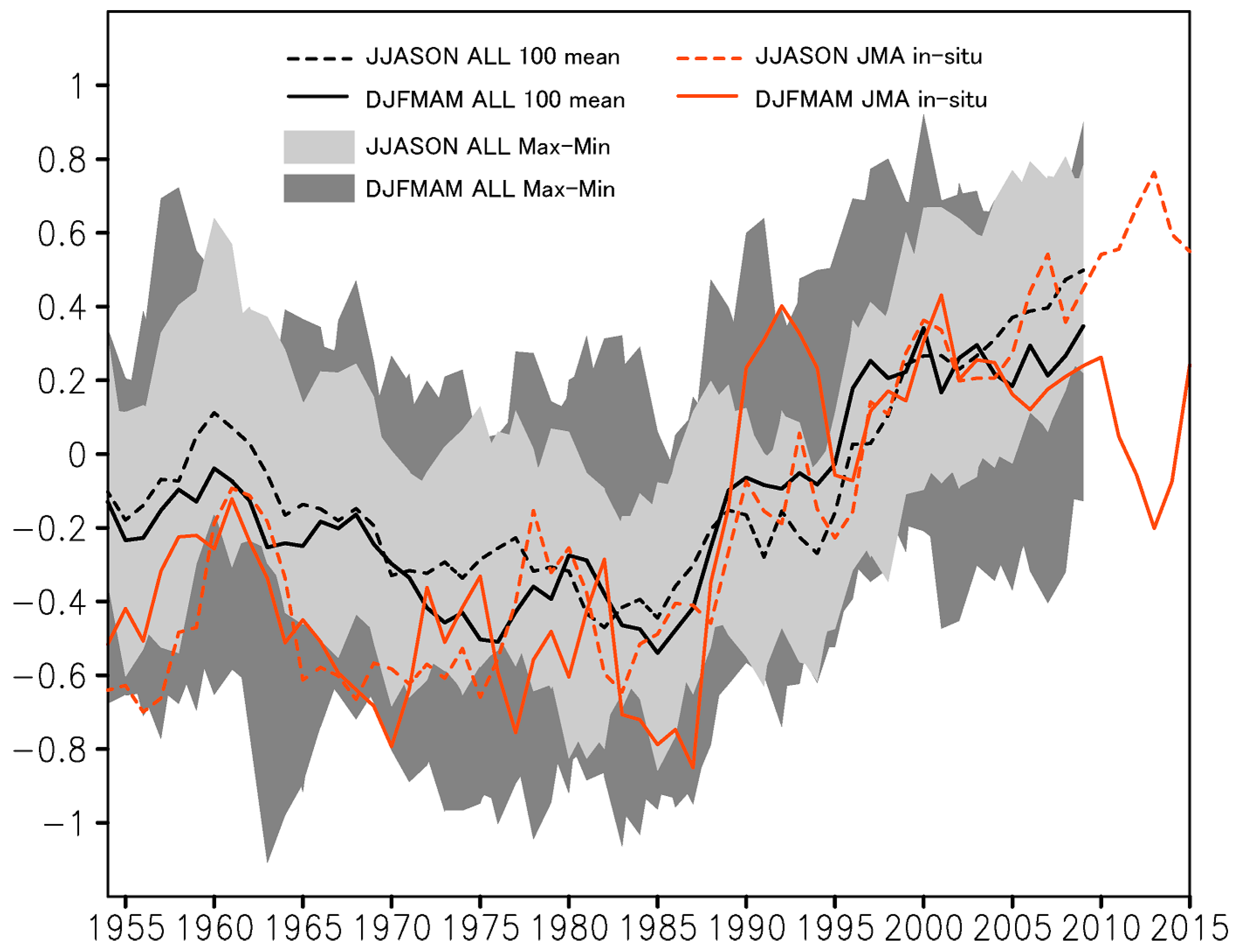
3.1. Historical Changes in the Surface Temperature of Japan

Time series of surface air temperature anomalies in Japan smoothed by five-year running means were compared with the JMA in-situ observations and the ALL run (Figure 1). In the observation (Figure 1a), post-2000 temperatures showed an increasing trend during the summer and autumn, and a decreasing trend during the winter and spring. Urabe and Maeda [1] attributed these trends to seasonally-different teleconnection patterns in atmospheric circulation responding to enhanced convective activity around the western equatorial Pacific, which has been associated with decadal-scale La Nina-like conditions since the late 1990s (Figure 2a,b).

The ensemble mean of our historical simulation (the ALL run) reproduced well the enhanced seasonal temperature contrast in Japan in the 21st century (Figure 1). There were some differences in the early years (before the 1970s) between the observation and the 100-menber mean, indicating smaller trend or multi-decadal variation in the model. One possible reason is that the model result is ensemble mean value, while the observation includes noises even in a decadal timescale. The range of the ensemble member covers most of the observed values through the years of the experiment. Over narrow islands like Japan, SST surrounding the islands can affect the land surface temperature changes. Although there is a possibility that SST given to the AGCM limits fluctuations in land surface temperature, the wide range among the simulated members shown in Figure 1 indicates that atmospheric variation is a main driver for surface temperature in mid-latitudes. The simulated ensemble-mean temperature also captured the warm winter/spring and cold summer/autumn conditions from the late 1980s to the early 1990s. This period corresponded to the decade when the IPO phase changed from negative to positive. The positive IPO (decadal El Nino-like condition) might affect the seasonal temperature contrast in Japan during this period, although few studies have examined the effect. In this study, we focus more on the changes in the 2000s.

From observational data alone, it was unclear whether the observed trend represented external forcing agents, SST changes, and/or occasional events due to atmospheric natural variability, however, through our ensemble-mean time series, we were able to reduce atmospheric noise and confirm that the signals in seasonal differences during the 2000s are a response to anthropogenic and natural external forcing including SST and sea ice variations given as boundary conditions.

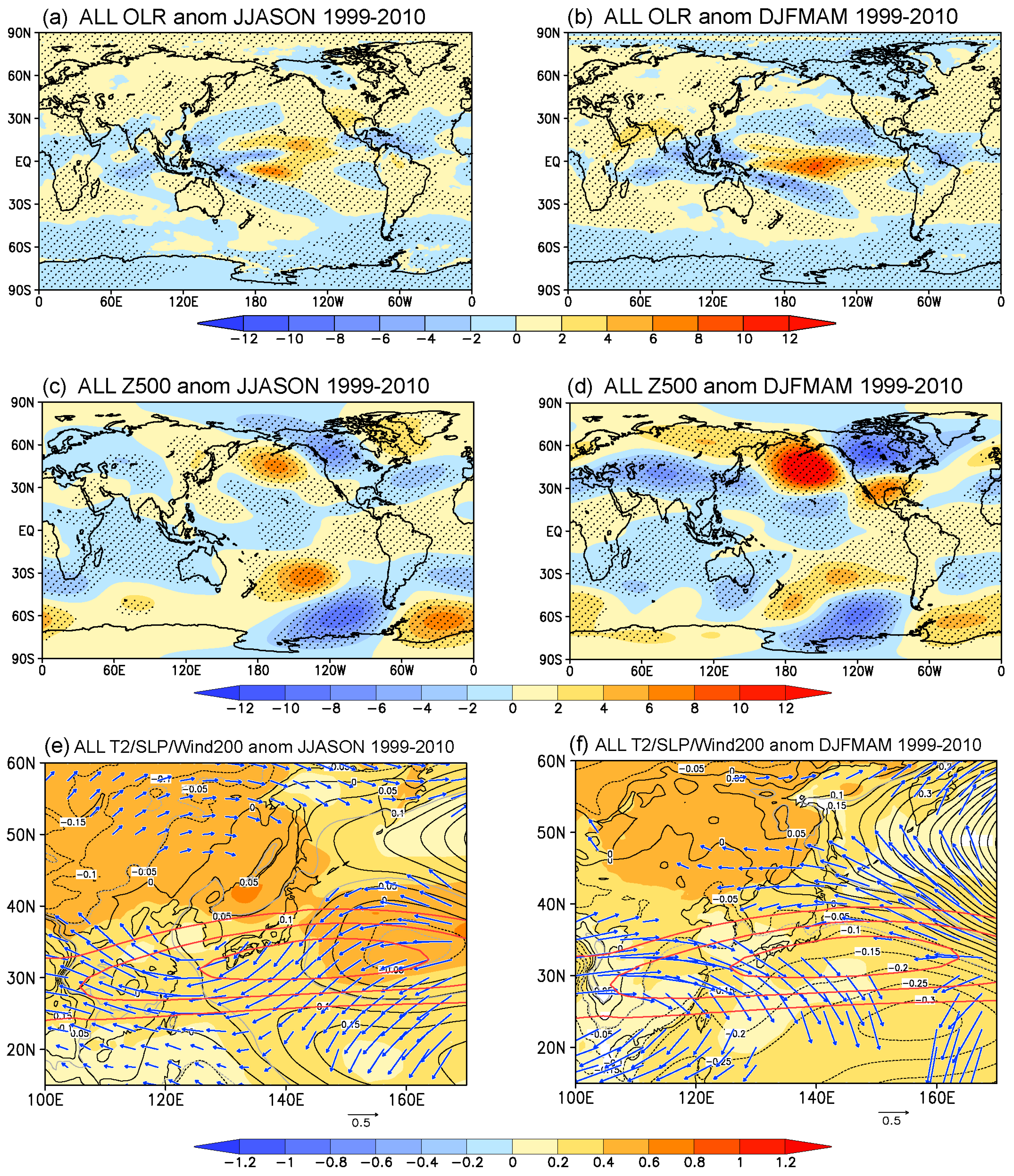
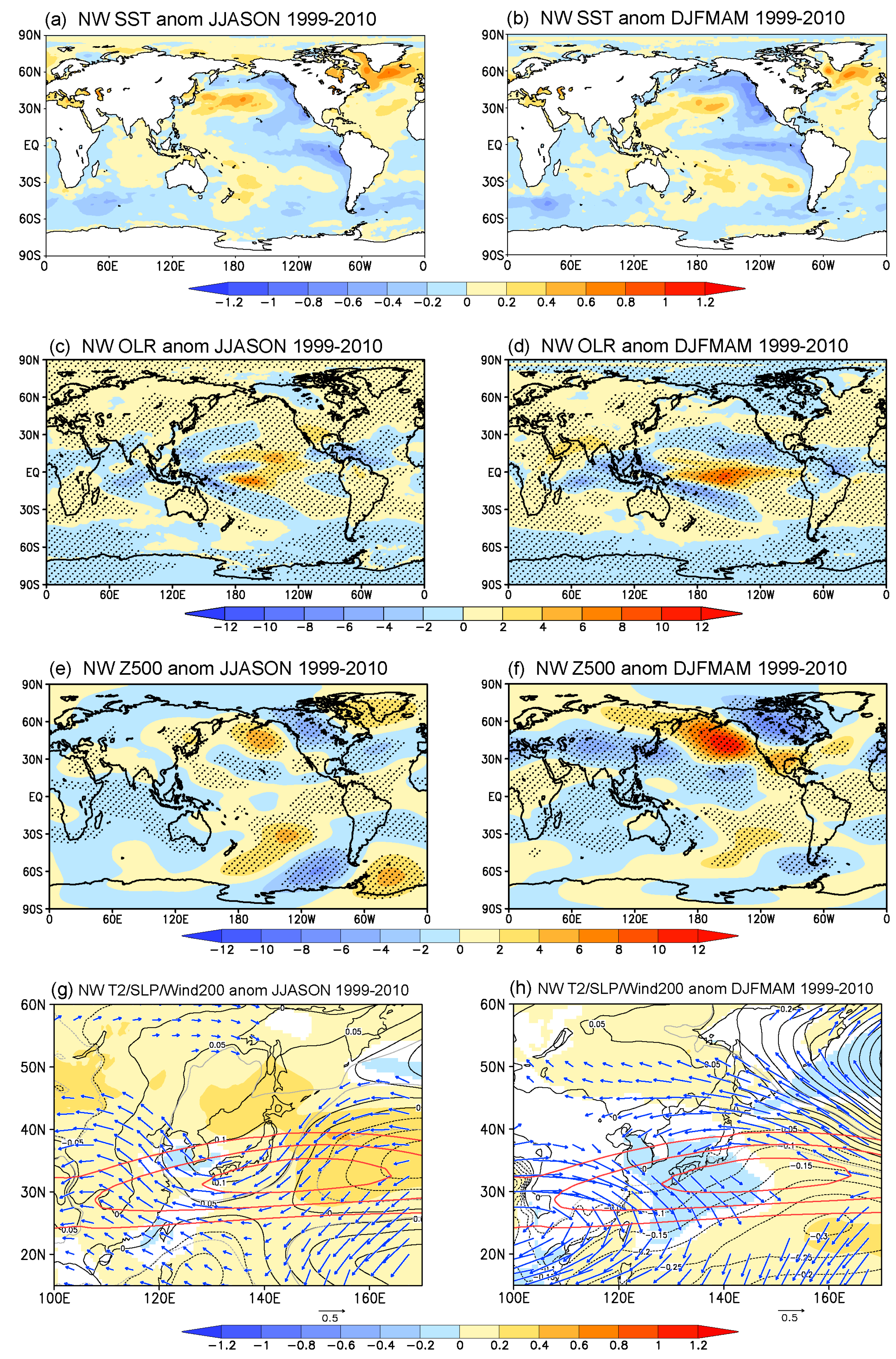
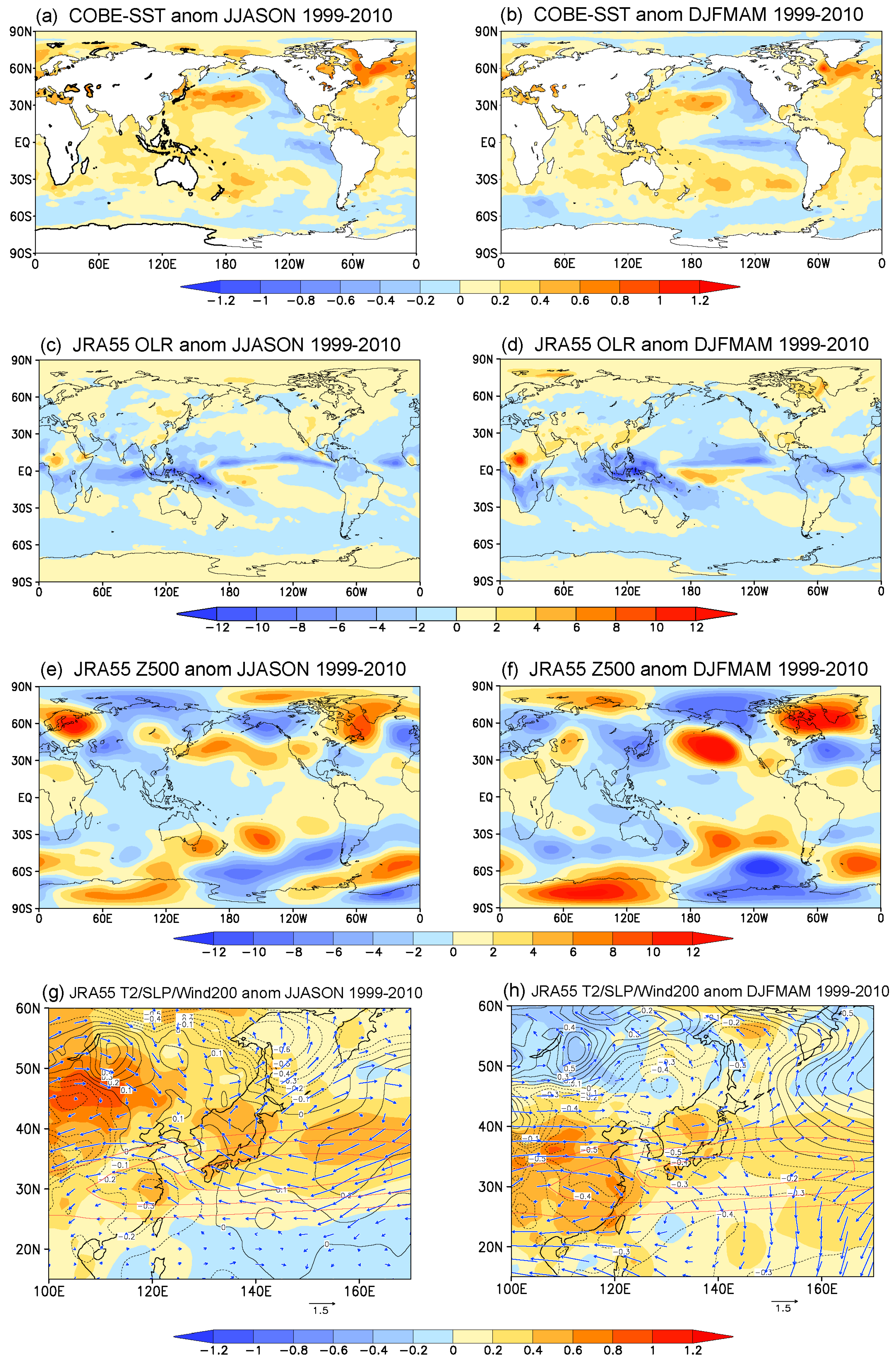
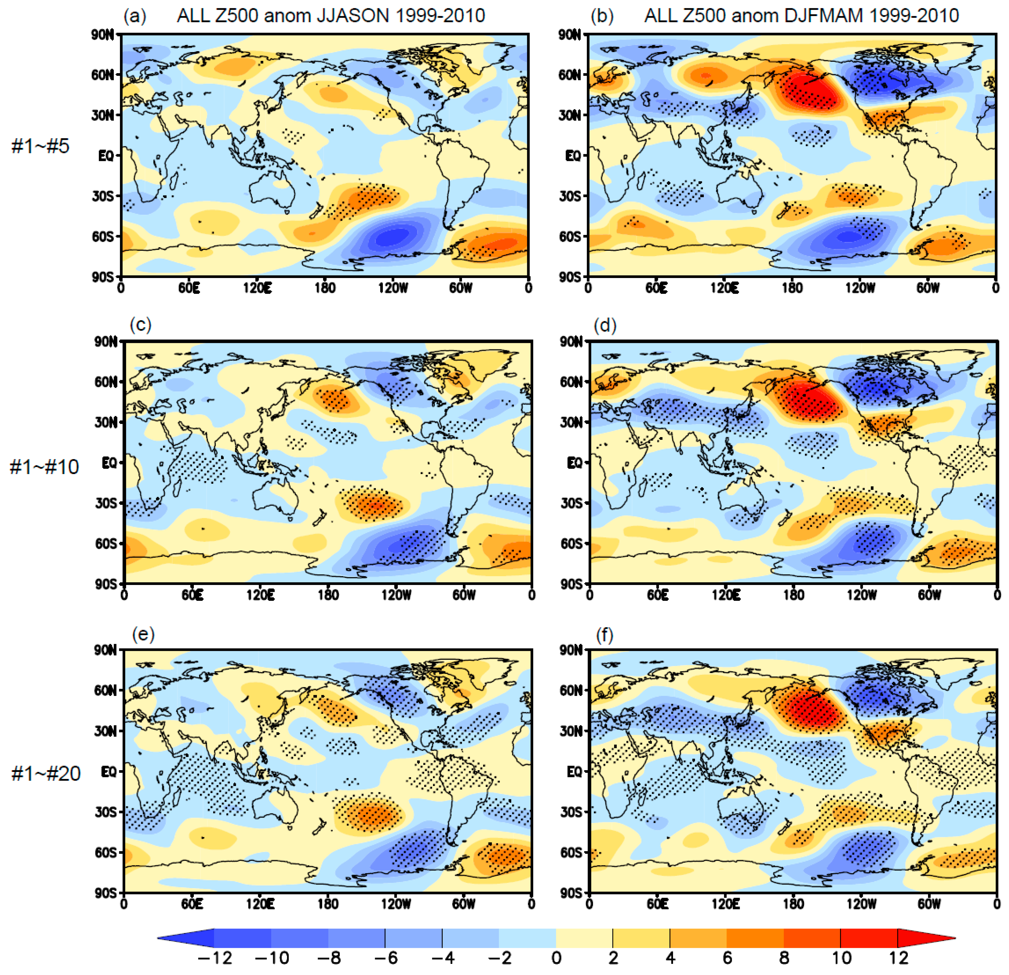
3.2. Atmospheric Anomalies in the 2000s

In observed SST anomalies of JJASON and DJFMAM averaged from 1999 to 2010, La Nina-like conditions were observed in the tropical Pacific, while warm anomalies were distributed east of Japan (Figure 2a,b). This pattern is typical of a negative phase of IPO. Here, the global warming trends relative to the reference period (1981–2010) are included in Figure 2. Associated with the La Nina-like SST anomalies, negative outgoing longwave radiation (OLR) anomalies were visible in the western Pacific (Figure 2c,d), indicating enhancement of convection over the Maritime Continent and Walker circulation in both seasons. The enhanced convective activity in the western equatorial Pacific was the source of a Rossby wave-like train on a decadal timescale, especially from December to May. The wave pattern was observed in 500 hPa geopotential height (Z500) anomalies (Figure 2f). It made barotropic cyclonic anomaly (negative Z500 and sea level pressure (SLP) anomalies in Figure 2f,h) from eastern Eurasia to Japan, which brought colder air in DJFMAM in Japan [1]. In contrast, from June to November, zonally elongated positive anomalies were visible from East Asia to North America (Figure 2e), and were also related to active convection in the western tropical Pacific [1]. The positive Z500 anomalies over Japan corresponded to a northward shift of the Asian Jet and the enhanced Pacific High (200-hPa wind velocity and SLP anomalies in Figure 2g), and resulted in higher temperatures. Relatively, the cyclonic anomaly in DJFMAM suppressed recent warming and the anticyclonic anomaly in JJASON enhanced warming, resulting in an increase in seasonal contrast in the early 21st century around Japan. Here, the 3-month mean anomalies of JJA and SON (DJF and MAM) were relatively similar to JJASON (DJFMAM) and contributed to the results in Figure 2 (not shown).

The ALL run captured the enhanced convective activity in the western equatorial Pacific (Figure 3a,b) and positive (negative) Z500 anomalies over Japan in JJASON (DJFMAM) (Figure 3c,d), a northward shift of the Asian Jet in JJASON and barotropic cold-cyclonic anomalies in DJFMAM, resulting in the warmer JJASON anomalies compared to the DJFMAM anomalies (Figure 3e,f) around Japan, as identified in observational data. There are some discrepancies between the ensemble-mean values and the observation (e.g., land surface temperature and Z500 in the north Eurasia), suggesting a possibility that the observed anomalies in those regions were part of atmospheric internal variability. The ensemble-mean Z500 anomalies averaged from 1999 to 2010 contained Rossby wave responses from the western equatorial Pacific to North America in DJFMAM, and zonally elongated positive anomalies from East Asia to North America in JJASON (Figure 3c,d). The results clearly highlight the importance of large ensemble size, especially in the extratropics, to isolate forced signals from stochastic internal variability. We conducted a Student’s t-test and found that where only 5 or 10 ensemble members were used, anomalies in the extratropics were less significant (Figure 4a–d, 99% significance level) because large atmospheric intrinsic variability in mid-latitudes suppresses the signals of the atmospheric responses to SST and sea ice variability, which are given as a bottom boundary condition of the AGCM. On the other hand, anomalies become 99% statistically significant across most of the globe when the ensemble size increases to 100 (Figure 3c,d), at which point most atmospheric intrinsic variability is compensated for, and significant signals remain after averaging the anomalies of the 100 members. From this perspective, our large ensemble database represents a powerful tool for investigating meaningful signals that have been obscured by atmospheric noise in observational data.

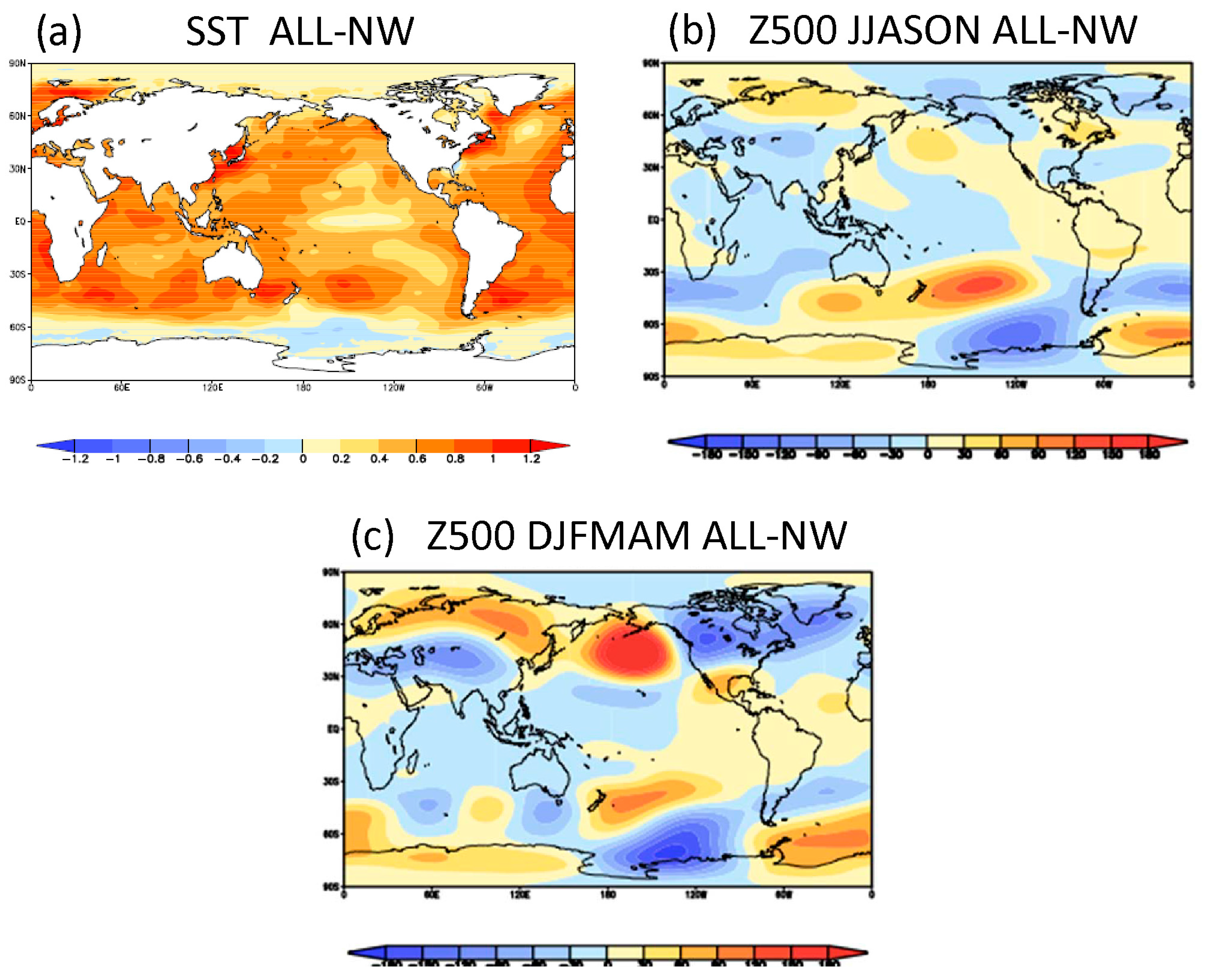
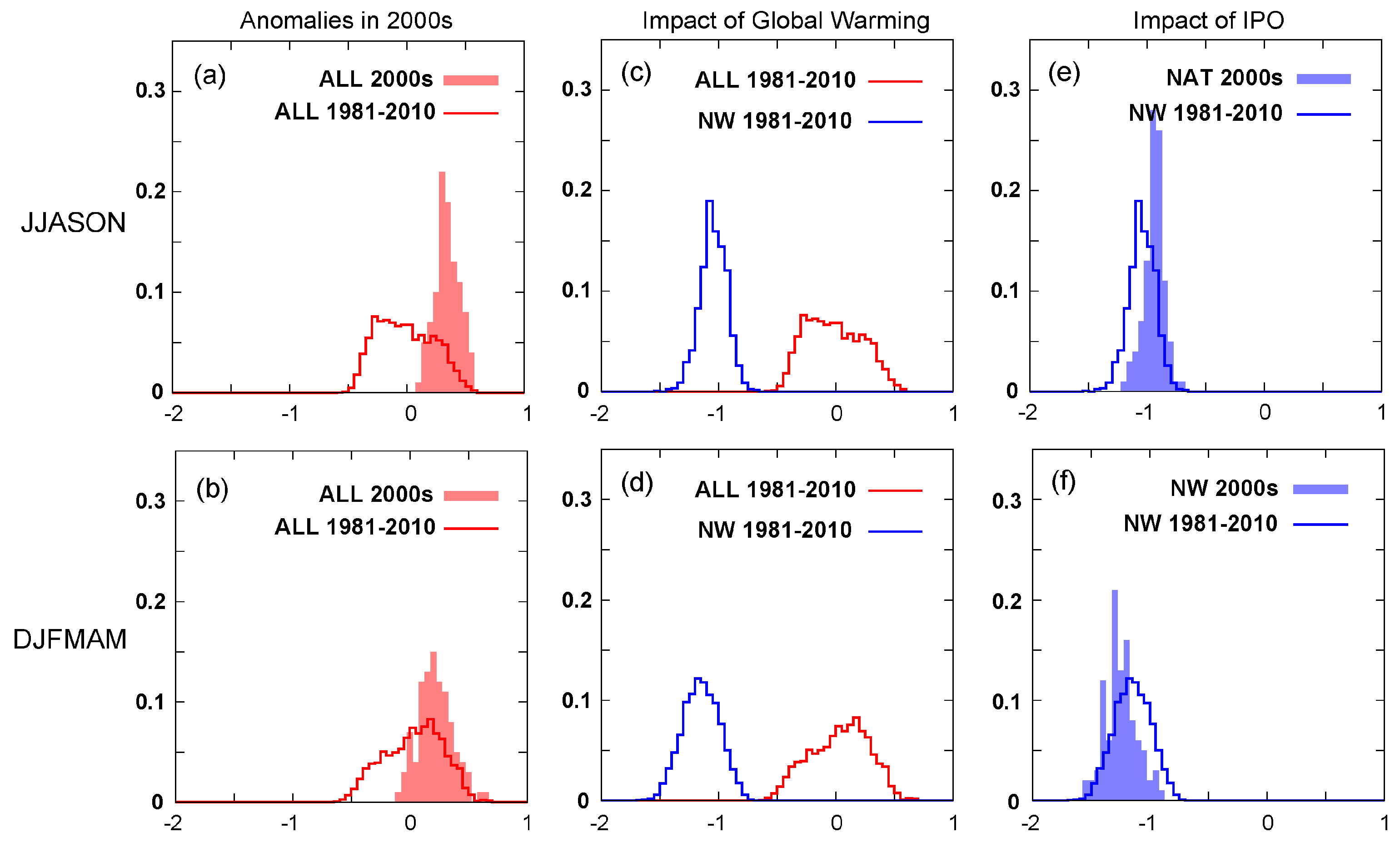
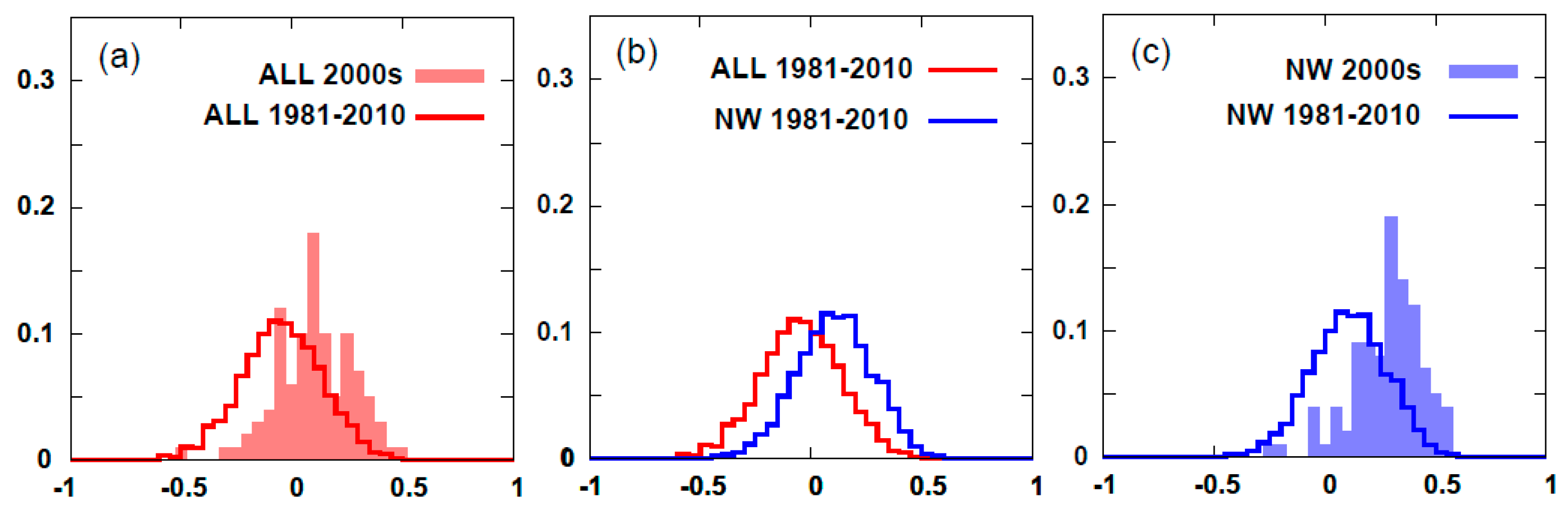
3.3. Attribution Study

Temperature anomalies in Japan in both observational data and ALL simulations result from the global warming, long-term natural variability in SST and sea ice, and atmospheric intrinsic variability. Atmospheric intrinsic variability can be expressed as the spread among ensemble members and was compensated for by taking the ensemble mean. To isolate impacts of long-term natural variability in boundary forcing, we compared the results of the NW and ALL runs.

We compared histograms of 12-year mean temperatures after 1999 to every 12-year window in the reference period (1981–2010) using the ALL run (Figure 5a,b) and found that warm anomalies in Japan became more frequent after 1999, both in JJASON and in DJFMAM. Again, this reflects both anthropogenic climate change and natural variability in boundary forcing. To isolate the effects of anthropogenic warming, we compared histograms of 12-year-mean temperature data from the ALL run and NW run (Figure 5c,d) and found that there is no doubt about the impacts of anthropogenic climate change on the increase in warm periods over Japan both in JJASON and in DJFMAM. The impact of decadal natural variability was examined using the NW run by comparing post-1999 anomalies with anomalies during the reference period (Figure 5e,f). The results showed that in comparison with the reference period, warmer (colder) periods in JJASON (DJFMAM) become more frequent after 1999, which is consistent with the increasing seasonal temperature contrast.

To more precisely quantify the impacts of each factor on decadal-scale seasonal temperature contrast in Japan, we compared the differences in anomalous temperature between JJASON and DJFMAM (Figure 6). The ALL run showed that the differences were significantly more frequent after 1999 than they were over the whole reference period (Figure 6a). This positive shift can be attributed mainly to decadal natural variability (i.e., La Nina-like conditions during this period; Figure 6c). On the other hand, comparison between the ALL and NW run (Figure 6b) indicated a slightly negative shift of the distribution (reducing seasonal differences) due to anthropogenic global warming (Figure 6b).

In the NW run, ensemble-mean anomalies averaged from 1999 to 2010 did not exhibit warming trends and atmospheric intrinsic variability was almost compensated for by taking the ensemble mean (Figure 7). Owing to the large ensemble approach, the atmospheric anomalies met a 99% statistically significant level almost everywhere, even in the extratropics (Figure 7c–f, based on a Student’s t-test). Positive (negative) temperature anomalies were visible around Japan in JJASON (DJFMAM). The circulation anomaly patterns showed the enhanced convective activity in the western equatorial Pacific (Figure 7c,d) and positive (negative) Z500 anomalies over Japan in JJASON (DJFMAM) (Figure 7e,f), a northward shift of the Asian Jet in JJASON (Figure 7g) and barotropic cold-cyclonic anomalies in DJFMAM (Figure 7h) around Japan, which were in agreement with observed features over the north Pacific shown in Figure 2. This confirms that observed anomaly patterns over East Asia during the 2000s were mainly the consequence of decadal scale Pacific variability.

We also considered the role of global warming in seasonal temperature differences over East Asia. The differences in annual mean SST between the ALL and NW runs, which corresponds to the defined global warming trend that was excluded from the NW run, showed that warming was faster in the Atlantic and Indian Oceans than in the Pacific Ocean (Figure 8a), and that warming was also faster around Japan. In the tropical Pacific Ocean, warming was faster in the west than in the east, which increased the mean zonal SST gradient. Here, seasonal differences in the ALL minus NW SST patterns were not apparent because we defined the global warming trend using annual mean SST. However, maps of Z500 responding to the boundary condition changes showed seasonal differences (Figure 8b,c), with positive Z500 anomalies occurring around Japan in DJFMAM, but with unclear changes in JJASON. This resulted in faster warming in DJFMAM than in JJASON, consistent with the smaller seasonal temperature contrast in Japan in the ALL run compared to the NW run (Figure 6b). This result is also consistent with the change tendency obtained from future projections of CMIP5 models [16].

4. Conclusions

In this study, we used large ensemble historical and counterfactual simulations to investigate increased seasonal temperature contrasts in Japan during the first decade of the 21st century. Each simulation contained 60-year records with 100 ensemble members, which reduced atmospheric noise and allowed us to investigate how atmospheric signals respond to boundary forcing. Previous large-ensemble simulations have been limited to recent years and focused on short-lived extreme events. By taking advantage of long-term datasets, this work provides a new attribution study focused on decadal-scale events.

The results show that increases in temperature contrast in Japan have mainly been induced by atmospheric anomalies responding to decadal La Nina-like conditions (i.e., negative IPO) in the tropical Pacific. In contrast, global warming has acted in the reverse, suppressing seasonal contrast. However, even though this opposite effect of global warming was considered, the influence of the negative IPO in the 2000s was large enough to increase the occurrence of the relatively warmer (colder) temperature in JJASON (DJFMAM).

A particular point of interest is the ensemble spread in 12-year mean data in Figure 5 and Figure 6 corresponding to atmospheric internal variability. This indicates that atmospheric intrinsic variability is not negligible on a decadal scale over East Asia. Deser et al. [18] showed that long-term variability associated with random stochastic processes has a significant impact and is comparable to external forcing and long-term natural variability at the initial stage of global warming. Therefore, in the future climate, if negative IPO and atmospheric perturbations coincide with global warming, Japan and other East Asian countries could face an increased risk of extremely high temperatures during the summer and autumn.

The results of this study still contain uncertainties; for example, global warming trends excluded from the boundary conditions of the AGCM in the NW simulations. Furthermore, discrepancies remain among the GCMs. To assess this uncertainty, future iterations of the NW simulation will incorporate multi-boundary conditions and multi-model approaches.

References

1. Urabe, Y.; Maeda, S. The relationship between Japan’s recent temperature and decadal variability. SOLA 2014, 10, 176–179. [Google Scholar] [CrossRef]
2. Zhang, Y.; Wallace, J.M.; Battisti, D.S. ENSO-like interdecadal variability. J. Clim. 1997, 10, 1004–1020. [Google Scholar] [CrossRef]
3. Power, S.; Casey, C.; Folland, C.; Colman, A.; Mehta, V. Inter-decadal modulation of the impact of ENSO on Australia. Clim. Dyn. 1999, 15, 319–324. [Google Scholar] [CrossRef]
4. Meehl, G.A.; Arblaster, J.M.; Fasullo, J.T.; Hu, J.; Trenberth, K.E. Model-based evidence of deep-ocean heat uptake during surface-temperature hiatus periods. Nat. Clim. Chang. 2011, 1, 360–364. [Google Scholar] [CrossRef]
5. Meehl, G.A.; Hu, A.; Arblaster, J.M.; Fasullo, J.; Trenberth, K.E. Externally forced and internally generated decadal climate vaeiability associated with the Interdecadal Pacific Oscillation. J. Clim. 2013, 26, 7298–7310. [Google Scholar] [CrossRef]
6. Kosaka, Y.; Xie, S.P. Recent global-warming hiatus tied to equatorial Pacific surface cooling. Nature 2013, 501, 403–407. [Google Scholar] [CrossRef] [PubMed]
7. Watanabe, M.; Kamae, Y.; Yoshimori, M.; Oka, A.; Sato, M.; Ishii, M.; Mochizuki, T.; Kimoto, M. Strengthening of ocean heat uptake efficiency associated with the recent climate hiatus. Geophys. Res. Lett. 2013, 40. [Google Scholar] [CrossRef]
8. Japan Meteorological Agency. El Nino and Japanese Climate. Available online: http://www.data.jma.go.jp/gmd/cpd/data/elnino/learning/tenkou/nihon1.html (accessed on 30 December 2016).
9. Maeda, S. ENSO and Japan’s climate. Meteorol. Res. Note 2014, 228, 167–179. (In Japanese) [Google Scholar]
10. Wu, L.; Cai, W.; Zhang, L.; Nakamura, H.; Timmermann, A.; Joyce, T.; McPhaden, M.J.; Alexander, M.; Qiu, B.; Visbeck, M.; et al. Enhanced warming over the global subtropical western boundary currents. Nat. Clim. Chang. 2012, 2, 161–166. [Google Scholar] [CrossRef] [Green Version]
11. Xie, S.-P.; Hu, K.; Hafner, J.; Tokinaga, H.; Du, Y.; Huang, G.; Sampe, T. Indian Ocean capacitor effect on Indo-western Pacific climate during the summer following El Nino. J. Clim. 2009, 22, 730–747. [Google Scholar] [CrossRef]
12. Imada, Y.; Shiogama, H.; Watanabe, M.; Mori, M.; Ishii, M.; Kimoto, M. The contribution of anthropogenic forcing to the Japanese heat waves of 2013. In “Explaining Extreme Events of 2013 from a Climate Perspective”. Bull. Am. Meteorol. Soc. 2014, 95, S52–S54. [Google Scholar]
13. Deser, C.; Phillips, A.S.; Alexander, M.A. Twentieth century tropical sea surface temperature trends revisited. Geophys. Res. Lett. 2010, 37, L10701. [Google Scholar] [CrossRef]
14. Tokinaga, H.; Xie, S.-P.; Deser, C.; Kosaka, Y.; Okumura, Y.M. Slowdown of the Walker circulation driven by tropical Indo-Pacific warming. Nature 2012, 491, 439–443. [Google Scholar] [CrossRef] [PubMed]
15. Christidis, N.; Stott, P.A. Change in the odds of warm years and seasons due to anthropogenic influence on the climate. J. Clim. 2014, 27, 2607–2621. [Google Scholar] [CrossRef]
16. Hirahara, S.; Ohno, H.; Oikawa, Y.; Maeda, S. Strengthening of the southern side of the jet stream and delayed withdrawal of Baiu season in future climate. J. Meteorol. Soc. Jpn. 2012, 90, 663–671. [Google Scholar] [CrossRef]
17. Lu, J.; Vecchi, G.A.; Reichler, T. Expansion of the Hadley cell under global warming. Geophys. Res. Lett. 2007, 34, L06805. [Google Scholar]
18. Deser, C.; Phillips, A.; Bourdette, V.; Teng, H. Uncertainty in climate change projections: The role of internal variability. Clim. Dyn. 2012, 38, 527–546. [Google Scholar] [CrossRef]
19. Mizuta, R.; Murata, A.; Ishii, M.; Shiogama, H.; Hibino, K.; Mori, N.; Arakawa, O.; Imada, Y.; Yoshida, K.; Aoyagi, T.; et al. Over 5000 years of ensemble future climate simulations by 60 km global and 20 km regional atmospheric models. Bull. Am. Meteorol. Soc. 2016. [Google Scholar] [CrossRef]
20. Data Integration and Analysis System Program. Available online: http://www.diasjp.net/en/ (accessed on 17 March 2017).
21. Imada, Y.; Shiogama, H.; Watanabe, M.; Mori, M.; Ishii, M.; Kimoto, M. Contribution of anthropogenic circulation change to the 2012 heavy rainfall in southern Japan. In “Explaining Extreme Events of 2012 from a Climate Perspective”. Bull. Am. Meteorol. Soc. 2013, 94, S52–S54. [Google Scholar]
22. Outline NWP March. 2007. Available online: http://www.jma.go.jp/jma/jma-eng/jma-center/nwp/outline-nwp/index.htm (accessed on 30 December 2016).
23. Mizuta, R.; Yoshimura, H.; Murakami, H.; Matsueda, M.; Endo, H.; Ose, T.; Kamiguchi, K.; Hosaka, M.; Sugi, M.; Yukimoto, S.; et al. Climate simulations using MRI-AGCM3.2 with 20-km grid. J. Meteorol. Soc. Jpn. 2012, 90A, 233–258. [Google Scholar] [CrossRef]
24. Hirahara, S.; Ishii, M.; Fukuda, Y. Centennial-scale sea surface temperature analysis and its uncertainty. J. Clim. 2014, 27, 57–75. [Google Scholar] [CrossRef]
25. Shiogama, H.; Imada, Y.; Mori, M.; Mizuta, R.; Stone, D.; Yoshida, K.; Arakawa, O.; Ikeda, M.; Takahashi, C.; Arai, M.; et al. Attributing historical changes in probabilities of record-breaking daily temperature and precipitation extreme events. SOLA 2016, 12, 225–231. [Google Scholar] [CrossRef]
26. Kobayashi, S.; Yukinari, O.; Yayoi, H.; Ebita, A.; Moriya, M.; Onoda, H.; Onogi, K.; Kamahori, H.; Kobayashi, C.; Endo, H.; et al. The JRA-55 reanalysis: General specifications and basic characteristics. J. Meteorol. Soc. Jpn. 2015, 93, 5–48. [Google Scholar] [CrossRef]
27. Japan Meteorological Agency. Monthly Temperature Anomaly in Japan. Available online: http://www.data.jma.go.jp/cpdinfo/temp/list/csv/mon_jpn.csv (accessed on 13 February 2017).
Figure 1. Time series of 6-month mean Japanese land surface temperature anomalies (K) for June–November (JJASON; dashed line) and December–May (DJFMAM; solid line) from the Japan Meteorological Agency (JMA) in-situ observations (red) and 100-member mean of the large ensemble simulations of the ALL (“all forcing”) run (black). A five-year running mean is applied for each time series. Shading shows the range of the ensemble members.
Atmosphere 08 00057 g001
Figure 2. Observed anomalies averaged from 1999 to 2010 for DJFMAM (left) and JJASON (right). (a,b) sea surface temperature (SST) (K), (c,d) outgoing longwave radiation (OLR) (W/m2), (e,f) Z500 (m, zonal mean is removed), (g,h) surface air temperature (shading, K), sea level pressure (SLP; contours, hPa), and 200 hPa wind velocity (arrows, m/s). Red contours in (g,h) show 50, 60, and 70 m/s of climatological westerly as a reference of a mean position of the Asian Jet. Sea surface temperature (SST) is based on COBE-SST, and atmospheric variables are from JRA-55 reanalysis.
Atmosphere 08 00057 g002
Figure 3. One hundred-member ensemble-mean anomalies of the all-forcing (ALL) run averaged from 1999 to 2010 for JJASON (left) and DJFMAM (right). (a,b) OLR (W/m2), (c,d) Z500 (m, zonal mean is removed), (e,f) surface air temperature (shading, K), SLP (contours, hPa), and 200 hPa wind velocity (arrows, m/s). In (ad), dotted areas show values exceeding the 99% confidence level. In (e,f), red contours show 50, 60, and 70 m/s of climatological westerly as a reference of a mean position of the Asian Jet, and gray contours show the 99% confidence level of SLP. Values exceeding the 99% confidence level are shown for surface air temperature and 200 hPa wind anomalies.
Atmosphere 08 00057 g003
Figure 4. Z500 anomalies of the ALL run (m, zonal mean is removed) averaged from 1999 to 2010 for JJASON (left) and DJFMAM (right). Ensemble average is calculated for randomly-chosen 5 members (a,b), 10 members (c,d), and 20 members (e,f). Dotted areas show values exceeding the 99% confidence level.
Atmosphere 08 00057 g004
Figure 5. Histograms of 12-year-mean Japanese land surface temperature anomalies of JJASON (a,c,e) and DJFMAM (b,d,f). The histograms are normalized by each sample number. Open columns are for each 12 year window from 1981 to 2010, and filled columns are averaged from 1999 to 2010. Red (blue) is results from the ALL (non-warming; NW) run. (a and b) comparison of 1999–2010 with 1981–2010 based on the ALL run, (c and d) comparison of ALL with NW, (e and f) comparison of 1999-2010 with 1981–2010 based on the NW run.
Atmosphere 08 00057 g005
Figure 6. Same as Figure 5, but for the difference of temperature anomalies between JJASON and DJFMAM (JJASON minus DJFMAM). (a) comparison of 1999–2010 with 1981–2010 based on the ALL run, (b) comparison of ALL with NW, (c) comparison of 1999-2010 with 1981–2010 based on the NW run.
Atmosphere 08 00057 g006
Figure 7. One hundred-member ensemble-mean anomalies of the NW run averaged from 1999 to 2010 for JJASON (left) and DJFMAM (right). (a,b) OLR (W/m2), (c,d) Z500 (m, zonal mean is removed), (e,f) surface air temperature (shading, K), SLP (contours, hPa), and 200 hPa wind velocity (arrows, m/s). Red contours in (e,f) show 50, 60, and 70 m/s of climatological westerly as a reference of a mean position of the Asian Jet. In (cf), dotted areas show values exceeding the 99% confidence level. In (g,h), red contours show 50, 60, and 70 m/s of climatological westerly as a reference of a mean position of the Asian Jet, and gray contours show the 99% confidence level of SLP. Values exceeding the 99% confidence level are shown for surface air temperature and 200 hPa wind anomalies.
Atmosphere 08 00057 g007
Figure 8. Differences between the ALL and NW run averaged from 1981 to 2010 (ALL minus NW). (a) Annual SST (K); (b) Z500 [m] for JJASON; (c) Z500 (m) for DJFMAM. A 100-member mean is used.
Atmosphere 08 00057 g008