
Importance of Gaseous Elemental Mercury Fluxes in Western Maryland

1
Appalachian Laboratory, University of Maryland Center for Environmental Science, Frostburg, MD 21532, USA
2
Gas Technology Institute, Des Plaines, IL 60018, USA
*
Author to whom correspondence should be addressed.
Atmosphere 2016, 7(9), 110; https://doi.org/10.3390/atmos7090110
Submission received: 15 July 2016
/
Revised: 17 August 2016
/
Accepted: 19 August 2016
/
Published: 23 August 2016
Abstract
:The purpose of this study was to increase our understanding of the gaseous elemental mercury (GEM, Hg°) fluxes between the atmosphere and soils. Moreover, we wanted to quantify the annual GEM flux, identify the controls, and compare the GEM flux to annual rates of gaseous oxidized mercury (GOM) dry deposition and wet deposition of total mercury. We measured GEM fluxes using the modified Bowen ratio (MBR) technique from 6 July 2009 to 6 July 2010 in western Maryland. The annual hourly mean (±std. dev.) GEM flux was −0.63 ± 31.0 ng·m−2·h−1. Hourly mean GEM fluxes were not strongly correlated with atmospheric trace gases, aerosols, or meteorology. However, hourly mean GEM emissions (15.3 ± 27.9 ng·m−2·h−1) and deposition (−14.6 ± 26.6 ng·m−2·h−1) were correlated with ultraviolet-B radiation (UV-B), wind speed (WS), ozone (O3), and relative humidity (RH). The annual net GEM flux was −3.33 µg· m−2·year−1 and was similar to the annual dry deposition rate of GOM (2.5 to 3.2 µg·m−2·year−1), and 40% less than the annual mean wet deposition (8 µg·m−2·year−1) of total mercury. Thus, dry deposition of GEM accounted for approximately 25% of the total annual mercury deposition (~14 ug·m−2·year−1) measured at our study site.
1. Introduction
Surface-atmosphere exchange of GEM can be important to the overall biogeochemical cycling of mercury [1,2,3,4]. Studying this exchange is often difficult due to the relatively small concentration gradients, low surface-atmosphere fluxes, and rapid changes in the direction of the flux. GEM, which comprises up to 95% of total atmospheric gaseous mercury, can be emitted from and deposited to soils [3,5]. This bi-directional movement can happen quickly, with a site switching between being a source and a sink of GEM within a few hours [6,7]. This important flux has been measured with flux chambers and micrometeorological techniques. However, few studies have measured this flux for an entire year [4,7,8]. Due to the high variability of GEM fluxes, it is necessary to make long-term measurements in order to determine the factors controlling these fluxes, which may vary widely throughout the year [3].
Many environmental parameters have been shown to influence this surface—atmosphere GEM exchange. Some of these factors include UV-B radiation, WS, and O3 concentrations [9,10,11,12,13]. UV-B radiation is thought to increase the photo-reduction of GOM (Hg2+) to GEM in the shallow soil layers [9,12]. This GEM is volatile and may be readily emitted to the atmosphere. Therefore, increased UV-B radiation may lead to increased GEM emissions. Higher wind speeds and turbulence near the soil surface have also been shown to increase the turbulent transfer of GEM, leading to higher exchange at higher wind speeds [13,14]. Ambient air O3 may increase GEM deposition in some environments or increase GEM emissions in others. For example in Polar Regions, atmospheric mercury depletion events are believed to be caused by the oxidation of GEM to GOM by species, such as O3 or bromine [15,16,17]. However, in one lab study with soils amended with GEM and Hg2+, oxidizers such as O3 were shown to increase the conversion of GOM to GEM and/or increase the volatilization of GEM from soils [10]. The variability of these factors that control GEM fluxes also contributes to the erratic nature of the atmospheric fluxes.
Due to the variability of GEM fluxes and limited field measurements, we know very little about long-term variations and the importance of this flux in the mercury biogeochemical cycle. We also still do not fully understand how different factors influence these fluxes. Therefore, one goal of our study was to continuously measure GEM fluxes for one year at a site in western Maryland. The second goal was to put our annual GEM flux into perspective with other annual mercury fluxes measured at the same site. A third goal was to identify factors that strongly influenced the GEM fluxes.
2. Experimental Section
2.1. Site Description
GEM fluxes were measured almost continuously from 6 July 2009 to 6 July 2010 at the Piney Reservoir ambient air monitoring station (PRAAMS) in Garrett County Maryland (39°42′21.29′′N, 79°0′43.21′′W). PRAAMS is located on a relatively flat, high elevation (781 m) ridge top adjacent to the Piney Creek Reservoir and is surrounded primarily by deciduous forests (Figure 1). In 2004, we cleared the ridge top, and we now measure a diverse suite of atmospheric trace gases, aerosols and meteorological parameters (Table 1). For this study, we also measured soil redox, soil temperature, soil moisture, leaf surface wetness, total UV, UV-B, net solar radiation, albedo, wind speed and wind direction. Our flux tower was located 30 m to the west of the equipment shelters (Figure 1). We chose this location in order to have the greatest amount of fetch (upwind distance of uniform roughness) from the west to north, which is the predominant wind direction. PRAAMS is also known as MD08, a monitoring station in the National Atmospheric Deposition Program’s National Trends Network (NADP NTN), NADP’s Mercury Deposition Network (NADP MDN) and the Atmospheric Mercury Network (AMNet). A detailed description of PRAAMS can be found in [18]. There are relatively few atmospheric mercury sources within 50 km of PRAAMS, but several sources within 150 km [19].
Mean annual air temperature for the entire campaign was 8.5 °C, roughly equal to the long-term (1972–2010) annual mean temperature of 8.8 °C [20]. For our measurement period, precipitation was 136.0 cm, the 5th highest since 1972 and snowfall was 260.9 cm, the 13th highest since 1972 (20). The long-term annual average precipitation and snowfall for PRAAMS was 114.2 cm, and 212.6 cm, respectively. PRAAMS was at least partially snow covered from 20 December 2009 to 25 March 2010. Soils were classified as Dekalb and Gilpin very stony loams and had a mean total mercury concentration of 0.05 µg of mercury per g of soil [21,22].
2.2. Modified Bowen Ratio
The MBR method was used to measure the GEM fluxes [4,7,13,23,24,25]. This is a micrometeorological technique that combines high-speed (10 Hz) eddy correlation and GEM concentration gradient measurements. The eddy correlation measurements were used to measure the kinematic heat flux with a 3D ultrasonic anemometer (R.M. Young 81000VRE). The ultrasonic anemometer was mounted at 2 m and was between two sets of thermistors that were mounted at 1 m and 3 m above the ground. We then used the kinematic heat flux and the temperature gradient measured between the thermistors at 1 and 3 m to calculate a vertical transport term (K) that was applied to the GEM gradient to determine the flux. In this way we were using heat as a reference scalar in order to determine the movement of GEM. By using heat as a reference scalar, we assumed that the transport of GEM was controlled by the same vertical mixing phenomena as the transport of heat. We chose temperature and heat flux as the reference scalars instead of CO2 or water vapor, to eliminate some of the problems experienced by others under dry and low CO2 conditions [7]. K was calculated with Equation (1):
where w’T’ was the kinematic heat flux (K·m·s−1) and ΔT (K) was the hourly difference in temperature between 1 and 3 m.
The GEM flux was then determined with Equation (2):
where FGEM was the GEM flux (ng·m−2·h−1) and ΔCGEM was the hourly GEM concentration gradient between 1 m and 3 m. To determine the hourly GEM and temperature gradients, the hourly mean at the lower height was subtracted from the hourly mean at the upper height.
The dry deposition velocity (Vd) for GEM was then determined using Equation (3):
where FGEM was the GEM flux (ng·m−2·h−1) and CGEM is the concentration of GEM at the 3 m height. This deposition velocity was used for comparison with previous estimates.
GEM concentrations were measured with a Tekran 2537A Mercury Vapor Analyzer (2537A) located in a temperature-controlled building approximately 30 m from the flux tower. The 2537A continuously measured GEM concentrations by switching between two gold traps. Mercury was collected on one gold trap (A channel) for five minutes, then while the mercury was being desorbed and analyzed from the A channel, mercury was being collected by another gold trap (B channel). The 2537A had a detection limit of <0.1 ng·m−3 [26]. To determine the GEM concentrations at 1 and 3 m, two identical-length 3/16” ID Teflon tubing, one from each height, were attached to a Tekran Model 1110 synchronized two port sampling system, which was attached to the 2537A. The 1110 automatically switched between the two inlets every 15 min (three 5 min sampling periods). The first five-minute sample was discarded during data analysis to prevent skewing of the data due to stagnant air in the 30 m Teflon tubing. Flows into the 2537A were maintained at 1.0 L·min−1 using a mass flow controller and were checked monthly with a Bios DryCal Definer 220 flow meter.
The temperatures at each height were measured every minute with two 1000 Ω platinum resistance thermistors (PRTs) inside Met One 076B aspirated shields. These shields allowed consistent air flow across the PRTs and removed them from direct sunlight and precipitation. The precision of the PRTs was ±0.01 °C. The temperature gradient was calculated by subtracting the hourly mean of the two PRTs at 3 m from the hourly mean of the two PRTs at 1 m.
2.3. GEM Measurements
The 2537A was automatically calibrated from an internal calibration system every 49 h. The analyzer was closely monitored and taken offline or serviced if the difference between the gold traps (channels A and B) rose above 7.5%. The 2537A was offline 749 of 9234 h over our annual measurement period for calibration, maintenance, power failures, or use on other projects. Twice during the year, the accuracy of the internal calibration source was examined by several injections of GEM from a Tekran 2505 mercury calibration unit and a digital syringe (1702RN, 25 µL, Hamilton Co., Reno, NV, USA). Both times, the accuracy of internal calibration system was within the uncertainty of the permeation rate. The sample inlet on the back of the 2537A had a 2 µm Teflon filter, which removed particles and gaseous oxidized mercury. Therefore, GEM was the only gaseous species of mercury that entered the analyzer.
To be certain we were measuring real GEM gradients with our flux tower, we set both sampling inlets at 1 m, six times throughout the measurement campaign (Table 2). This allowed us to compare data from periods of collocated inlets to periods when inlets were separated by 2 m. This comparison was necessary in order to determine the GEM concentration gradient threshold that was caused by real variation in the GEM concentrations rather than measurement uncertainties. We also placed the PRTs at the same 1 m height during these six periods. By doing this, we were able to determine that one of the four PRTs was measuring 0.1 °C higher than the three other PRTs. Therefore, 0.1 °C was always subtracted from this PRT before any flux calculation.
2.4. Statistical Analyses
All statistical analyses were performed using the R Project for statistical computing (version 2.10.1) on hourly mean values. Pearson Product Moment correlations were significant at an α = 0.05. ANOVA was used to determine significant differences in mean GEM fluxes by season and wind direction sector and the differences in mean emission and deposition by season. A Tukey’s HSD test was used with the ANOVA results to test for significant differences amongst seasons. Spectral and partial autocorrelation function analyses were used to evaluate our filtered GEM fluxes. Spectral analysis was used to identify any characteristic time frequency of variation in GEM fluxes. The partial autocorrelation function analysis was used to determine if subsequent hours were correlated. In order to perform the spectral and partial autocorrelation function analysis, we performed linear interpolations to fill in missing data for 749 h out of our total sampling of 9234 h. These data were missing due to the 2537A being offline for calibration periods, flow measurements, routine maintenance, or the weather prevented the ultrasonic anemometer from working properly.
2.5. Flux Footprint
The flux footprint is the upwind area that contributes to the GEM flux measured at our tower. We estimated the flux footprint using the model developed by [27]. This model has been widely used by other researchers to estimate flux footprints [4,28,29,30]. Input for this model included our hourly measurements of sensible heat flux (H), air temperature, and friction velocity (u*). Canopy height, zero plane displacement, and momentum roughness were defined as 0.5 to 1.0 m (depending on season), 0.335 m, and 0.05 m, respectively. Zero plane displacement and momentum roughness were estimated from [31].
We used this model to calculate the direction and fetch where 80% of the GEM flux occurred. The last 20% of the footprint can extend for hundreds to thousands of meters with only a small contribution to the flux. The model results were separated into periods of stable, neutral, and unstable atmospheric conditions. Unstable conditions occurred when the Monin-Obukhov lengths (z·L−1) were less than −0.02. In contrast, stable conditions occurred when the Monin-Obukhov lengths were greater than 0.02. Neutral conditions were the transition period between stable and unstable [27]. Note that z is the measurement height and L is the Obukhov length [27,31].
2.6. GEM Flux Validation
Our GEM fluxes were calculated, in part, from the GEM concentration gradient between the 1 and 3 m measurement heights (Equation (2)). We wanted to determine the GEM concentration gradient threshold caused by real differences in GEM concentrations between these two heights, rather than measurement uncertainties. In other words, we wanted to define a GEM concentration difference threshold to discard data caused by measurement uncertainties. To do this, we examined the variation in the GEM concentrations when the two inlets were collocated at 1 m (Table 2). The overall mean difference for these collocated periods was 0.006 ng·m−3 and the range was −0.004 to 0.016 ng·m−3 (Table 2). From these collocation periods, we selected two possible gradient thresholds, 0.009 ng·m−3 and 0.016 ng·m−3.
To determine the more effective threshold, we examined the absolute value of the GEM concentration difference between the two inlets for the entire measurement campaign. By using the absolute value we avoided comparing GEM gradients that could have been biased low by the many positive and negative values. To demonstrate this, the mean GEM gradient when the inlets were separated was −0.003 ± 0.045 ng·m−3 and ranged from −0.281 to 0.570 ng·m−3. On the other hand, the mean absolute value for the same data was 0.034 ± 0.029 ng·m−3. For the entire data set, there was no significant difference (p = 0.5232) between the mean absolute values (0.034 ± 0.029 ng·m−3 vs. 0.035 ± 0.029 ng·m−3) when the inlets were apart and co-located at 1 m. When we removed concentration gradients less than 0.009 ng·m−3, the difference in mean absolute values became significant (p = 6.83 × 10⁻⁶). The mean GEM gradient, during separated periods, increased to 0.040 ± 0.030 ng·m−3. As a result, all fluxes with concentration gradients less than 0.009 ng·m−3 were removed from our data set (18% of total data). Filtering at a threshold of 0.016 ng·m−3 also produced a significant difference between collocated and separated periods but would have removed 32% of the fluxes. The later threshold was not used because it removed more data than the 0.009 ng·m−3 threshold. Below we refer to our unfiltered and filtered fluxes. Our unfiltered fluxes contain the entire data set and the filtered fluxes include only the fluxes from GEM concentration gradients greater than the 0.009 ng·m−3 threshold.
To be more certain that the GEM fluxes were not simply random noise, we performed a time series analysis on our filtered data. The partial autocorrelation function (PACF) of the annual time series revealed that the fluxes were correlated for five hours (Figure 2). This indicated that even though the fluxes were noisy, subsequent hours, up to 5 h, were correlated. If the fluxes had been noise alone, then they would not have been autocorrelated. We also performed a spectral analysis on the fluxes. We did not find a characteristic frequency of variation, such as every 24 or 168 h that would indicate a distinct daily or weekly variation. However, the spectrum was not a flat line, which would have indicated random noise. Collectively, our filtered data contained real fluxes generated by real differences in the GEM concentration gradient.
Finally, there were two buildings located 30 m east of our flux tower. To determine the effects of these buildings on our measurements, we divided the fluxes into eight wind direction sectors (45 degree sections of the 360 degree wind rose). We looked for significant differences in the average flux for each sector. For the entire measurement campaign, GEM fluxes were not significantly different among the eight wind direction sectors. This indicated that the buildings did not artificially bias our GEM fluxes.
3. Results and Discussion
3.1. GEM Fluxes
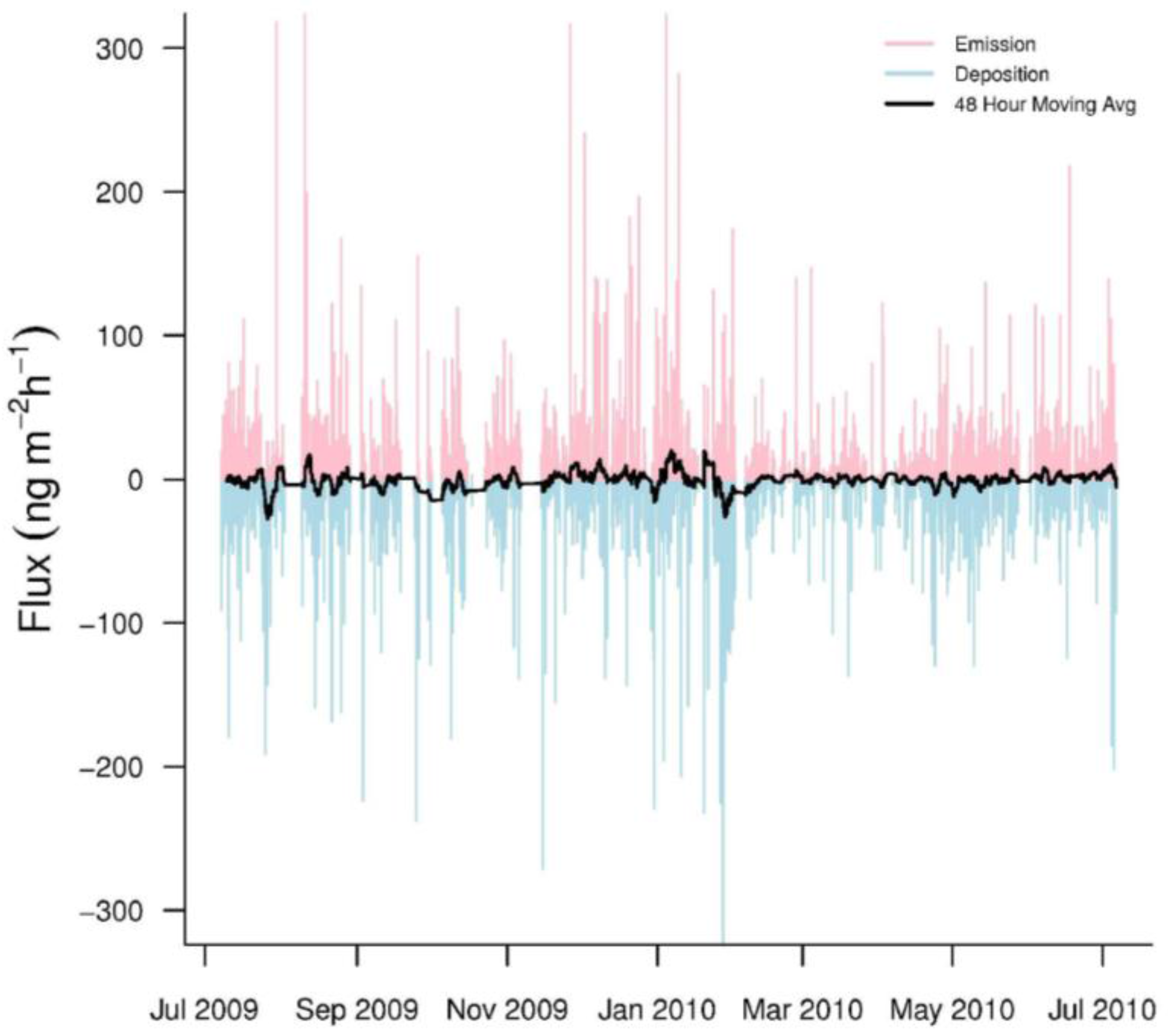
Hourly GEM fluxes were highly variable, switching between emission and deposition (Figure 3). The mean hourly GEM flux was −0.63 ± 31.0 ng·m−2·h−1 (n = 5259). In addition, our seasonal mean GEM fluxes were consistently negative, indicating that GEM dry deposition was common at PRAAMS (Table 3). The range (−346.1 to 379.8 ng·m−2·h−1) of our measured fluxes over the year was much larger than other studies especially in the winter (Table 3). The only other study to come close to this range was over a mixed wetland, vegetation, and open water system [5]. This could indicate that the vegetation, topography, land uses and/or unknown processes within our flux footprint sporadically caused large variations in the GEM fluxes. In addition, previous studies with short measurement periods, may not have sampled enough to capture these extreme variations.
The net GEM flux for the year was −3.33 ug·m−2·year−1 for the filtered fluxes. The net GEM flux for the unfiltered fluxes (all GEM gradients included) was −3.74 ug·m−2·year−1. This indicates that the GEM fluxes below our threshold made a small contribution to the overall net flux. Note that the net negative fluxes occurred because the dry deposition (negative fluxes) of GEM at PRAAMS was greater than the emissions (positive fluxes) of GEM into the atmosphere. Our filtered seasonally mean GEM fluxes were not significantly different amongst seasons. However, the greatest and most frequent GEM emissions and deposition tended to occur in fall and early winter. From February through April, GEM emissions and deposition at PRAAMS were much lower compared to other times of the year.
To determine the source area of our GEM flux measurements throughout the year, we examined our flux footprint model results. For our entire measurement campaign, the atmospheric stability conditions were 25.7% unstable, 45.7% neutral and 28.6% stable. During unstable conditions, the mean footprint for 80% of the GEM flux was within 200 m of our flux tower. During neutral conditions, the mean footprint for 80% of the GEM flux was within 300 m of flux tower. During stable conditions, mean footprint for 80% of the GEM flux was within 2000 m from our flux tower. For 71.4% of our entire sampling campaign, 80% of the GEM flux was within 300 m of our tower. The vegetation within that 300 m was mostly grasses and brush with a few dispersed trees (Figure 1).
In order to put our study into perspective with others, we calculated the GEM deposition velocity (Vd). The Vd is often used by modelers to estimate atmospheric deposition of GEM [36]. Our annual mean Vd was 0.33 ± 0.61 cm·s−1 and ranged from 0 to 8.08 cm·s−1. Our mean Vd was in agreement with the mean Vd reported for vegetated surfaces and wetlands (0.1 to 0.4 cm·s−1) [36]. In spring, Vd (0.22 ± 0.33 cm·s−1) was significantly lower than summer (0.38 ± 0.71 cm·s−1), fall (0.38 ± 0.63 cm·s−1) and winter (0.31 ± 0.66 cm·s−1). Summer, fall and winter were not significantly different from each other. This pattern was also reported by the authors of [7]. The range of GEM fluxes at PRAAMS was also smaller in spring (Table 3). This indicated that there was less exchange of GEM between the surface and atmosphere during this season. The vegetation may have been less effective at removing GEM from the atmosphere during the onset of the growing season. Our range of Vd values were also more consistent with the range of Vd for forest canopies (0.0003 to 1.88 cm·s−1) than bare soils (0.002 to 0.064 cm·s−1) [36]. This could indicate that the forests at PRAAMS were important sinks for atmospheric GEM.
Mean hourly GEM fluxes were significantly but weakly (r < 0.05) correlated with mean hourly NO2, NOy, soil redox at 5 cm into the E horizon and total UV. The fluxes were not related to any of the 25 other variables measured. Therefore, we were not able to identify any factors that consistently influenced the GEM fluxes.
3.2. GEM Emission and Deposition
Due to the low correlation coefficients between the GEM fluxes and all of the other measured variables, we examined the GEM emission and deposition separately [13]. Annual mean GEM emission was 15.3 ± 27.9 ng·m−2·h−1 (n = 2453). Mean GEM emissions in spring (12.9 ± 21.1 ng·m−2·h−1), summer (16.8 ± 29.8 ng·m−2·h−1) and winter (13.9 ± 29.8 ng·m−2·h−1) were not significantly different. However, mean GEM emissions fall (17.8 ± 29.4 ng·m−2·h−1) were significantly higher than the mean GEM emission in spring. GEM emissions were also greater under unstable atmospheric conditions (23.8 ± 28.4 ng·m−2·h−1) than under neutral (21.5 ± 33.1 ng·m−2·h−1) or stable (3.00 ± 5.43 ng·m−2·h−1) conditions. Our mean GEM emission was slightly higher than the emission (7.5 ± 7.0 ng·m−2·h−1) from the Walker Branch Watershed in Oak Ridge, TN [13]. However, this study was limited to short daytime sampling periods from May through November 1994.
Annual mean GEM deposition was −14.6 ± 26.6 ng·m−2·h−1 (n = 2806). Mean GEM deposition in the spring (−11.4 ± 17.3 ng·m−2·h−1) was significantly lower than summer (−15.5 ± 27.3 ng·m−2·h−1), fall (−16.6 ± 21.1 ng·m−2·h−1) and winter (−15.2 ± 32.5 ng·m−2·h−1). Deposition for the year was also significantly higher under unstable atmospheric conditions (−23.0 ± 29.7 ng·m−2·h−1) than under neutral (−17.5 ± 29.3 ng·m−2·h−1) or stable (−3.3 ± 10.5 ng·m−2·h−1) atmospheric conditions. Our GEM deposition was also higher than the mean daytime GEM deposition (−2.2 ± 2.4 ng·m−2·h−1) at the Walker Branch Watershed [13].
Separating the fluxes into emission and deposition revealed that several variables were influencing the fluxes. However, most of the correlation coefficients were still below 0.25 (Table 4). By looking at only the variables with the highest correlation coefficients in each season, we were able to draw a few conclusions. UV-B was correlated with emission in summer, fall and spring and with deposition in summer and spring (Table 4). Although more strongly related than other parameters, UV-B still only explained 22% of the variation of the GEM emissions (in summer) and 17% of the deposition (in spring). However, we did find that as UV-B increased, emissions increased and deposition decreased. This was consistent with the findings of others and may indicate that UV-B photo-reduction of GOM to GEM at the soil surface may have been influencing the GEM fluxes [9,12,37]. This was also in agreement with our findings that high soil pore concentrations of GEM were causing a concentration gradient driven GEM flux [22]. It was possible that the conversion between GOM and GEM occurring at or near the soil surface was an important factor influencing GEM fluxes throughout the year.
The importance of the conversion between GOM and GEM occurring at the soil surface was also supported by correlations with ambient air O3 concentrations in summer. As O3 concentrations increased, GEM emission increased and deposition decreased. This relationship was consistent with the findings of the authors of [10], who reported that GEM emissions increased from soils enriched in bound Hg2+ under higher ambient air O3 concentrations (up to ~70 ppb). Although they did not determine the exact mechanism, they speculated that the O3 was oxidizing sulfur species, such as HgS, and this oxidation was counterbalanced by the reduction of Hg2+ (gaseous or bound) in the soil matrix to GEM. The GEM was then emitted to the atmosphere. It was possible that this process was occurring at PRAAMS. However, we could not rule out the fact that higher UV-B also produced more local O3. Ozone can be produced in the troposphere from a photochemical reactions driven by UV-B radiation [38].
There were also higher GEM emissions and lower GEM deposition at higher wind speeds. The influence of wind speed on GEM fluxes indicates that greater air turbulence above the soil surface most likely altered the GEM gradient near the surface which in turn resulted in greater GEM emissions into the atmosphere. This would agree with our findings that both emissions and deposition were higher under unstable atmospheric conditions. As turbulence near the surface increased, the physical movement of the GEM increased. This further emphasized the importance of the soil surface even during periods when UV-B and O3 were lower, like in the fall and winter.
RH appeared to be a factor controlling emission and deposition during the warmer spring and summer months. Higher RH led to lower emissions and higher deposition. This was similar to that seen by other studies [7,39,40,41]. This relationship may indicate that increased moisture in the air could facilitate the oxidation of GEM to GOM and increase deposition.
3.3. Comparison with Other Measurements at PRAAMS
Our MBR measurements of GEM flux were part of a larger study to better understand the atmospheric mercury cycle at PRAAMS. Other studies measured GEM fluxes with dynamic flux chambers [22], GOM deposition with ion exchange membranes [18], total mercury in litter fall deposition [42], and total mercury in wet deposition [43]. One of these projects also modeled GOM deposition [18]. Here, we present a comparison of our two GEM flux measurement campaigns (dynamic flux chambers vs MBR), and then we put these fluxes into perspective with the other mercury measurements made at PRAAMS.
The net annual GEM flux was very different between our dynamic flux chambers and the MBR method [22]. Using our flux chambers, we estimated a net emission of 5 to 12 µg·m−2·year−1. With the MBR method, we estimated a net deposition of 3.33 µg·m−2·year−1. This emphasized the differences between the measurement techniques. Fluxes measured with the MBR method were representative of a large area (footprint up to 2000 m2). The MBR fluxes were a summation of the soil, vegetation, and snow surfaces, and each surface may have had different factors controlling the GEM flux. Our chambers measured fluxes over a much smaller area (<0.5 m2). Flux chamber GEM fluxes could vary by two orders of magnitude within a single day in the forest and grass areas [22]. Additionally, there were periods when the soils beneath the chambers would switch from source to sink of GEM. This indicated that the landscape consisted of spatially variable GEM fluxes. As a result, to capture the variability within the MBR footprint, we would need to make many flux chamber measurements. The spatial variability of GEM fluxes may have been the reason we were not able to identify the factors correlated with MBR GEM fluxes. Therefore, we must be careful when scaling up fluxes measured with flux chambers to be representative of a large area. Our efforts verify the findings of others that micrometeorological and chamber fluxes do not agree [24].
Annual estimates of GOM deposition measured with ion exchange membranes and modeled using the multi-layer inferential model were 2.5 µg·m−2·year−1 and 3.2 µg·m−2·year−1 [18], respectively. These two estimates were essentially equal to the GEM dry deposition (3.3 ug·m−2·year−1) measured with the MBR technique. This indicates that dry deposition of GEM was as important as GOM deposition at PRAAMS. Historically, dry deposition of GEM was thought to be much smaller than the dry deposition of GOM [18,42]. Our measurements, however, suggest that the annual rates of GEM and GOM dry deposition are roughly equal at PRAAMS. Thus, dry deposition of GOM and GEM together accounted for about 5.8 to 6.5 ug·m−2·year−1 of mercury at PRAAMS.
Our dry deposition estimates of GOM and GEM together (5.8 to 6.5 µg·m−2·y−1) were roughly equal to the mean mercury wet deposition (7.6 µg·m−2·year−1) from 2004 to 2009 [43] at PRAAMS. Other studies have suggested that wet and dry deposition of mercury could be equal [44,45,46]. Our study verifies this assumption. Thus, the total mercury deposition at PRAAMS from GOM, GEM and wet deposition was around 14 ug·m−2·year−1, which is consistent with litterfall mercury (15 ug·m−2·year−1) inputs, and GEM accounted for approximately 25% of the total measured mercury deposition [42]. Thus, GEM plays an important role in mercury biogeochemical cycling at PRAAMS. Note, we did not include the dry deposition of particulate bound mercury in our calculations.
4. Conclusions
GEM fluxes at PRAAMS were very dynamic and not strongly correlated with atmospheric trace gases, aerosols, or meteorological variables. After separating our fluxes into periods of emission and deposition, we were able to determine that UV-B, O3, WS and RH influenced our GEM fluxes. However, even these relationships explained less than 22% of the variation in the GEM fluxes. This could indicate that parameters other than those measured were influencing the GEM fluxes at PRAAMS. These factors could include biological processes, variables that change on a shorter than one hour time scale, or variables that change substantially within the footprint of the flux tower. The few correlations could also indicate that we need to make higher resolution measurements of the possible GEM flux controls within the MBR flux footprint. Our comprehensive studies of mercury cycling at PRAAMS indicated that GEM deposition was as large as GOM deposition, and accounted for close to 25% of the total mercury deposition.
We suggest that future work should focus on improving our understanding of the role of O3 in GEM deposition and the importance of humidity on the atmospheric dynamics of GEM. In addition, we also suggest that future work focus on untangling the complexity of the variability of GEM fluxes within the MBR footprint.
Acknowledgments
This work was funded by the University of Maryland Center for Environmental Science. This publication has UMCES contribution number 5228.
Author Contributions
Both authors, Castro and Moore, contributed substantially to this this project. Castro and Moore conceived and designed this project; Moore performed the fieldwork; Moore and Castro analyzed the data; Moore operated and maintained the instrument, Castro helped when needed. Castro and Moore wrote this paper.
Conflicts of Interest
The authors declare no conflict of interest.
References
- Lindberg, S.; Bullock, R.; Ebinghaus, R.; Engstrom, D.; Feng, X.B.; Fitzgerald, W.; Pirrone, N.; Prestbo, E.; Seigneur, C. A synthesis of progress and uncertainties in attributing the sources of mercury in deposition. Ambio 2007, 36, 19–32. [Google Scholar] [CrossRef]
- Gustin, M.S.; Lindberg, S.E.; Weisberg, P.J. An update on the natural sources and sinks of atmospheric mercury. Appl. Geochem. 2008, 23, 482–493. [Google Scholar] [CrossRef]
- Gustin, M.; Jaffe, D. Reducing the uncertainty in measurement and understanding of mercury in the atmosphere. Environ. Sci. Technol. 2010, 44, 2222–2227. [Google Scholar] [CrossRef] [PubMed]
- Pierce, A.H.; Moore, C.W.; Wohlfahrt, G.; HÖrtang, L.; Kljun, N.; Obrist, D. Eddy covariance flux measurements of gaseous elemental mercury using cavity ring-down spectroscopy. Environ. Sci. Technol. 2015, 49, 1559–1568. [Google Scholar] [CrossRef] [PubMed]
- Poissant, L.; Pilote, M.; Beauvais, C.; Constant, P.; Zhang, H.H. A year of continuous measurements of three atmospheric mercury species (GEM, RGM and Hgp) in southern Quebec, Canada. Atmos. Environ. 2005, 39, 1275–1287. [Google Scholar] [CrossRef]
- Bash, J.O.; Miller, D.R. A relaxed eddy accumulation system for measuring surface fluxes of total gaseous mercury. J. Atmos. Ocean. Technol. 2008, 25, 244–257. [Google Scholar] [CrossRef]
- Converse, A.D.; Riscassi, A.L.; Scanlon, T.M. Seasonal variability in gaseous mercury fluxes measured in a high-elevation meadow. Atmos. Environ. 2010, 44, 2176–2185. [Google Scholar] [CrossRef]
- Baya, A.P.; Van Heyst, B. Assessing the trends and effects of environmental parameters on the behaviour of mercury in the lower atmosphere over cropped land over four seasons. Atmos. Chem. Phys. 2010, 10, 8617–8628. [Google Scholar] [CrossRef]
- Choi, H.D.; Holsen, T.M. Gaseous mercury emissions from unsterilized and sterilized soils: The effect of temperature and UV radiation. Environ. Pollut. 2009, 157, 1673–1678. [Google Scholar] [CrossRef] [PubMed]
- Engle, M.A.; Gustin, M.S.; Lindberg, S.E.; Gertler, A.W.; Ariya, P.A. The influence of ozone on atmospheric emissions of gaseous elemental mercury and reactive gaseous mercury from substrates. Atmos. Environ. 2005, 39, 7506–7517. [Google Scholar] [CrossRef]
- Gustin, M.S.; Taylor, G.E.; Maxey, R.A. Effect of temperature and air movement on the flux of elemental mercury from substrate to the atmosphere. J. Geophys. Res. Atmos. 1997, 102, 3891–3898. [Google Scholar] [CrossRef]
- Moore, C.; Carpi, A. Mechanisms of the emission of mercury from soil: Role of UV radiation. J. Geophys. Res. Atmos. 2005, 110, D24302. [Google Scholar] [CrossRef]
- Kim, K.H.; Lindberg, S.E.; Meyers, T.P. Micrometeorological measurements of mercury-vapor fluxes over background forest soils in Eastern Tennessee. Atmos. Environ. 1995, 29, 267–282. [Google Scholar] [CrossRef]
- Schluter, K. Review: Evaporation of mercury from soils. An integration and synthesis of current knowledge. Environ. Geol. 2000, 39, 249–271. [Google Scholar] [CrossRef]
- Hall, B. The gas-phase oxidation of elemental mercury by ozone. Water Air Soil Pollut. 1995, 80, 301–315. [Google Scholar] [CrossRef]
- Schroeder, W.H.; Anlauf, K.G.; Barrie, L.A.; Lu, J.Y.; Steffen, A.; Schneeberger, D.R.; Berg, T. Arctic springtime depletion of mercury. Nature 1998, 394, 331–332. [Google Scholar] [CrossRef]
- Steffen, A.; Douglas, T.; Amyot, M.; Ariya, P.; Aspmo, K.; Berg, T.; Bottenheim, J.; Brooks, S.; Cobbett, F.; Dastoor, A.; et al. A synthesis of atmospheric mercury depletion event chemistry in the atmosphere and snow. Atmos. Chem. Phys. 2008, 8, 1445–1482. [Google Scholar] [CrossRef] [Green Version]
- Castro, M.S.; Moore, C.W.; Sherwell, J.S.; Brooks, S.B. Dry deposition of gaseous oxidized mercury. Sci. Total Environ. 2011, 417, 232–240. [Google Scholar]
- Castro, M.S.; Sherwell, J. Effectiveness of emission controls to reduce the atmospheric concentrations of mercury. Envion. Sci. Technol. 2015, 49, 14000–14007. [Google Scholar] [CrossRef] [PubMed]
- SERCC. Southeastern Regional Climate Center. Available online: http://www.sercc.com/climateinfo/historical/historical_md.html (accessed on 22 August 2016).
- USDA. Web Soil Survey. Available online: http://websoilsurvey.nrcs.usda.gov/app/WebSoilSurvey.aspx (accessed on 22 August 2016).
- Moore, C.W.; Castro, M.S.; Heyes, A. Investigatioin of factors influencing gaseous mercury fluxes in background soils of western Maryland. Sci. Total Environ. 2011, 419, 136–143. [Google Scholar] [CrossRef] [PubMed]
- Fritsche, J.; Obrist, D.; Zeeman, M.J.; Conen, F.; Eugster, W.; Alewell, C. Elemental mercury fluxes over a sub-alpine grassland determined with two micrometeorological methods. Atmos. Environ. 2008, 42, 2922–2933. [Google Scholar] [CrossRef]
- Gustin, M.S.; Lindberg, S.; Marsik, F.; Casimir, A.; Ebinghaus, R.; Edwards, G.; Hubble-Fitzgerald, C.; Kemp, R.; Kock, H.; Leonard, T.; et al. Nevada STORMS project: Measurement of mercury emissions from naturally enriched surfaces. J. Geophys. Res. Atmos. 1999, 104, 21831–21844. [Google Scholar] [CrossRef]
- Lindberg, S.E.; Kim, K.H.; Meyers, T.P.; Owens, J.G. Micrometeorological gradient approach for quantifying air-surface exchange of mercury-vapor—Tests over contaminated doils. Environ. Sci. Technol. 1995, 29, 126–135. [Google Scholar] [CrossRef] [PubMed]
- Tekran. Model 2537A Mercury Vapor Analyzer User Manual. Available online: http://www.tekran.com/products/ambient-air/tekran-model-2537-cvafs-automated-mercury-analyzer/ (accessed on 22 August 2016).
- Hsieh, C.-I.; Katul, G.; Chi, T.W. An approximate analytical model for footprint estimation of scalar fluxes in thermally stratified atmospheric flows. Adv. Water Resour. 2000, 23, 765–772. [Google Scholar] [CrossRef]
- Oishi, A.C.; Oren, R.; Stoy, P.C. Estimating components of forest evapotranspiration: A footprint approach for scaling sap flux measurements. Agric. For. Meterol. 2000, 148, 1719–1732. [Google Scholar] [CrossRef]
- Park, S.J.; Park, S.U.; Ho, C.H.; Mahrt, L. Flux-gradient relationship of water vapor in the surface layer obtained from CASES-99 experiment. J.Geophys. Res. Atmos. 2009, 114, D08115. [Google Scholar] [CrossRef]
- Wohlfahrt, G.; Hortnagl, L.; Hammerle, A.; Graus, M.; Hansel, A. Measuring eddy covariance fluxes of ozone with a slow-response analyser. Atmos. Environ. 2009, 43, 4570–4576. [Google Scholar] [CrossRef] [PubMed]
- Arya, S.P. Introduction to Micrometeorology, 2nd ed.; Academic Press: San Diego, CA, USA, 2001. [Google Scholar]
- Lindberg, S.E.; Hanson, P.J.; Meyers, T.P.; Kim, K.H. Air/surface exchange of mercury vapor over forests—The need for a reassessment of continental biogenic emissions. Atmos. Environ. 1998, 32, 895–908. [Google Scholar] [CrossRef]
- Cobos, D.R.; Baker, J.M.; Nater, E.A. Conditional sampling for measuring mercury vapor fluxes. Atmos. Environ. 2002, 36, 4309–4321. [Google Scholar] [CrossRef]
- Fritsche, J.; Wohlfahrt, G.; Ammann, C.; Zeeman, M.; Hammerle, A.; Obrist, D.; Alewell, C. Summertime elemental mercury exchange of temperate grasslands on an ecosystem-scale. Atmos. Chem. Phys. 2008, 8, 7709–7722. [Google Scholar] [CrossRef] [PubMed] [Green Version]
- Poissant, L.; Pilote, M.; Constant, P.; Beauvais, C.; Zhang, H.H.; Xu, X.H. Mercury gas exchanges over selected bare soil and flooded sites in the bay St. Francois wetlands. Atmos. Environ. 2004, 38, 4205–4214. [Google Scholar] [CrossRef]
- Zhang, L.M.; Wright, L.P.; Blanchard, P. A review of current knowledge concerning dry deposition of atmospheric mercury. Atmos. Environ. 2009, 43, 5853–5864. [Google Scholar] [CrossRef]
- Xin, M.; Gustin, M.; Johnson, D. Laboratory investigation of the potential for re-emission of atmospherically derived Hg from soils. Environ. Sci. Technol. 2007, 41, 4946–4951. [Google Scholar] [CrossRef] [PubMed]
- Jacob, D.J.; Horowitz, L.W.; Munger, J.W.; Heikes, B.G.; Dickerson, R.R.; Artz, R.S.; Keene, W.C. Seasonal transition from NOx- to hydrocarbon-limited conditions for ozone production over the eastern United-States in September. J. Geophys. Res. Atmos. 1995, 100, 9315–9324. [Google Scholar] [CrossRef]
- Boudala, F.S.; Folkins, I.; Beauchamp, S.; Tordon, R.; Neima, J.; Johnson, B. Mercury flux measurements over air and water in Kejimkujik National Park, Nova Scotia. Water Air Soil Pollut. 2000, 122, 183–202. [Google Scholar] [CrossRef]
- Ericksen, J.A.; Gustin, M.S.; Xin, M.; Weisberg, P.J.; Fernandez, G.C.J. Air-soil exchange of mercury from background soils in the United States. Sci. Total Environ. 2006, 366, 851–863. [Google Scholar] [CrossRef] [PubMed]
- Poissant, L.; Casimir, A. Water-air and soil-air exchange rate of total gaseous mercury measured at background sites. Atmos. Environ. 1998, 32, 883–893. [Google Scholar] [CrossRef]
- Risch, M.R.; DeWild, J.F.; Krabbenhoft, D.P.; Kolka, R.K.; Zhang, L. Litterfall mercury dry deposition in the eastern USA. Environ. Pollut. 2012, 161, 284–290. [Google Scholar] [CrossRef] [PubMed]
- NADP. National Atmospheric Deposition Program 2009 Annual Summary; NADP Data Report 2009-01, Illinois State Water Survey; University of Illionois at Urbana-Champaign: Charpaign, IL, USA, 2010. [Google Scholar]
- Ryaboshapko, A.; Bullock, O.R.; Christensen, J.; Cohen, M.; Dastoor, A.; Ilyin, I.; Petersen, G.; Syrakov, D.; Artz, R.S.; Davignon, D.; et al. Intercomparison study of atmospheric mercury models: Comparison of models with short-term measurements. Sci. Total Environ. 2007, 376, 228–240. [Google Scholar] [CrossRef] [PubMed]
- Miller, E.K.; Vanarsdale, A.; Keeler, G.J.; Chalmers, A.; Poissant, L.; Kamman, N.C.; Brulotte, R. Estimation and mapping of wet and dry mercury deposition across northeastern North America. Ecotoxicology 2005, 14, 53–70. [Google Scholar] [CrossRef] [PubMed]
- Engle, M.A.; Tate, M.T.; Krabbenhoft, D.P.; Schauer, J.J.; Kolker, A.; Shanley, J.B.; Bothner, M.H. Comparison of atmospheric mercury speciation and deposition at nine sites across central and eastern North America. J. Geophys. Res. Atmos. 2010, 115, D18306. [Google Scholar] [CrossRef]
Figure 1.
The Piney Reservoir Ambient Air Monitoring Station (PRAAMS).
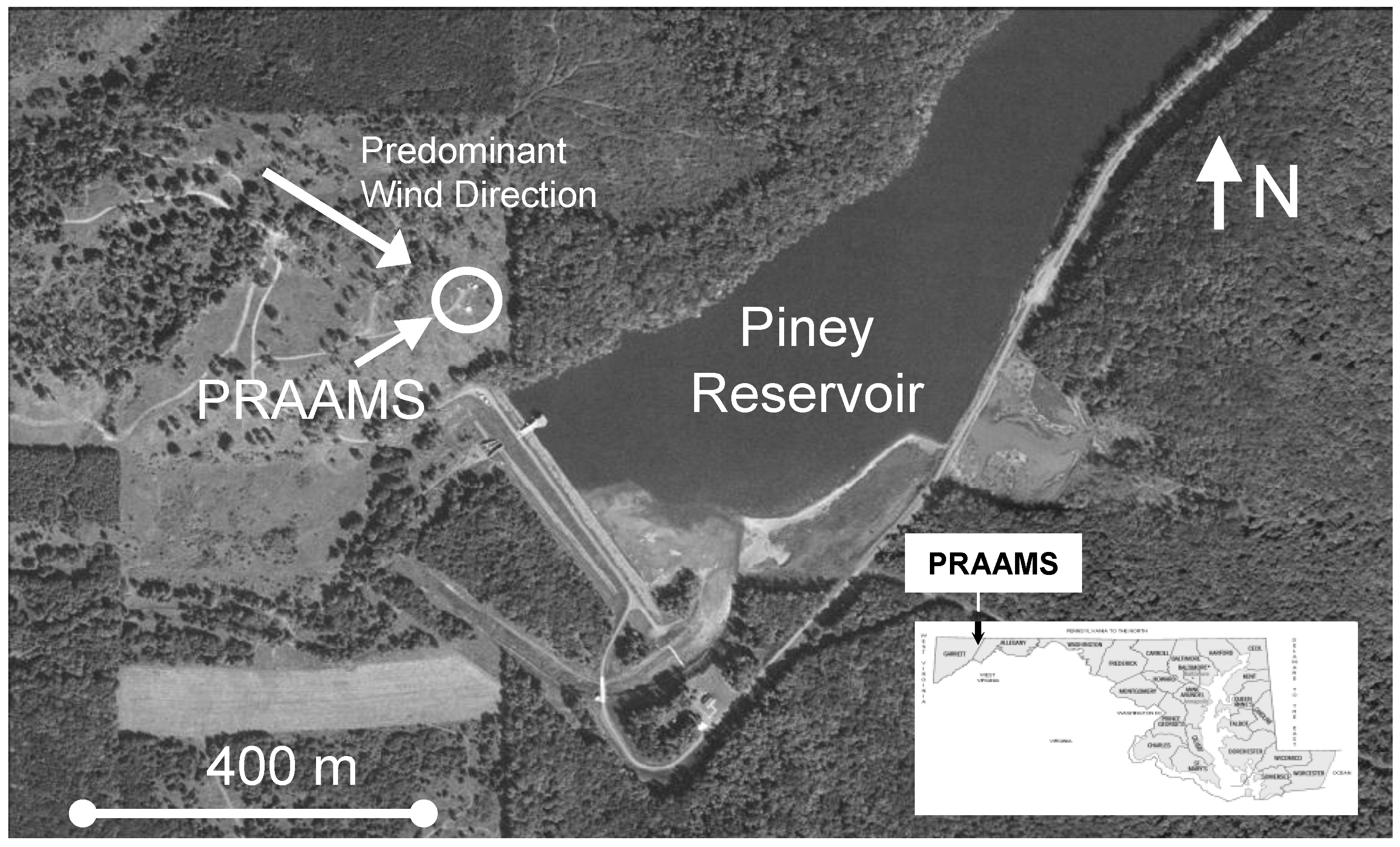
Figure 2.
The partial autocorrelation function (ACF) diagram of hourly GEM fluxes for the entire campaign. The dotted lines indicate the 95% confidence interval above or below hours significantly correlated with hour zero. The time lag on the x-axis is in units of hours and the Partial ACF on the y-axis in units of percent (%).
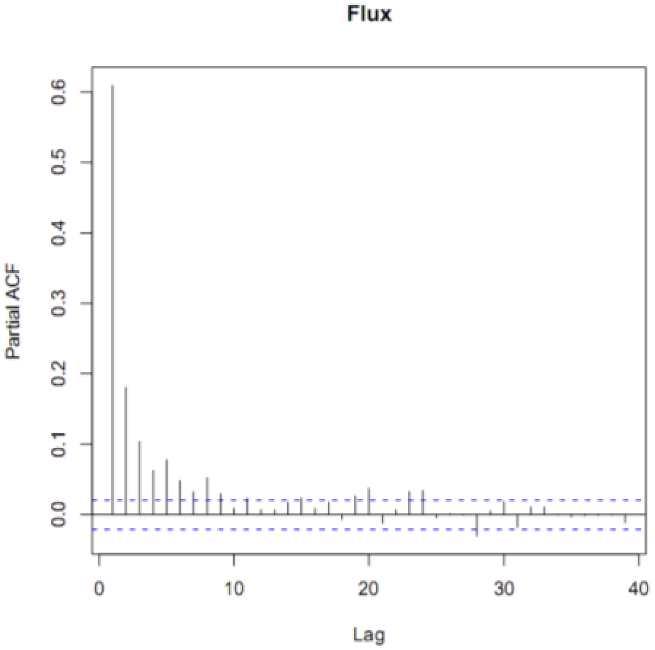
Figure 3.
Hourly GEM fluxes from July 2009 to July 2010. Emissions are pink while depositions are light blue. The black line represents a 48-h moving average of the hourly fluxes.
Figure 3.
Hourly GEM fluxes from July 2009 to July 2010. Emissions are pink while depositions are light blue. The black line represents a 48-h moving average of the hourly fluxes.

| Parameter | Frequency | Equipment |
|---|---|---|
| Soil Temperature | 10 Minutes | Decagon Devices 5TE |
| Soil Moisture | 10 Minutes | Decagon Devices 5TE |
| Soil Redox | 10 Minutes | Platinum wire probe |
| Total UV | 10 Minutes | Apogee Instruments SU-100 |
| UVB | 10 Minutes | Skye Instruments SKU 430 |
| Net Solar Radiation | 10 Minutes | Kipp and Zonen CNR-1 |
| Albedo | 10 Minutes | Kipp and Zonen CNR-1 |
| Ozone | 1 Hour | Thermo Electron 49C |
| CO | 1 Hour | Thermo Electron 58i-Tle |
| OCEC | 1 Hour | Sunset Labs 3F |
| SO2 | 1 Hour | Eco Tek EC9850t |
| NO | 1 Hour | Eco Tek EC9843 |
| NO2 | 1 Hour | Eco Tek EC9843 |
| NOy | 1 Hour | Eco Tek EC9843 |
| SO4 | 1 Hour | 5020 SPA Thermo |
| PM2.5 | 1 Hour | Met One Instruments BAM 1020 PM2.5 |
| Wind Speed (10 m) | 1 Hour | Vaisala WXT 520 |
| Wind Direction (10 m) | 1 Hour | Vaisala WXT 520 |
| Relative Humidity (RH) | 1 Hour | Vaisala WXT 520 |
| Air Temp (10 m) | 1 Hour | Vaisala WXT 520 |
| Dew point | 1 Hour | Calculated from Air Temp (10m) and RH |
| Rain | 1 Hour | Vaisala WXT 520 |
| Barometric Pressure | 1 Hour | Vaisala WXT 520 |
| Surface Wetness | 1 Hour | Cambell Scientific 237-L |
| Wind Speed (3 m) | 1 Hour | RM Young 05103 Wind Monitor |
| Wind Direction (3 m) | 1 Hour | RM Young 05103 Wind Monitor |
| GEM | 1 Hour | Tekran 2537 |
| GOM | 2 Hour | Tekran 1130 |
| Particulate Mercury | 2 Hour | Tekran 1135 |
| Start | End | Mean (GEM) Inlet 1 (ng·m−3) | Mean (GEM) Inlet 2 (ng·m−3) | Mean Difference | Maximum Gradient Magnitude | Minimum Gradient Magnitude | |
|---|---|---|---|---|---|---|---|
| Collocated | 26 June 2009 | 2 July 2009 | 1.199 | 1.190 | 0.009 | 0.086 | 0.000 |
| Collocated | 2 August 2009 | 9 August 2009 | 1.093 | 1.094 | 0.001 | 0.134 | 0.000 |
| Collocated | 29 August 2009 | 2 September 2009 | 1.024 | 1.008 | 0.016 | 0.125 | 0.000 |
| Collocated | 18 September 2009 | 23 September 2009 | 1.029 | 1.028 | 0.001 | 0.122 | 0.000 |
| Collocated | 6 November 2009 | 14 November 2009 | 1.532 | 1.534 | 0.008 | 0.110 | 0.000 |
| Collocated | 1 February 2010 | 5 February 2010 | 1.809 | 1.809 | 0.000 | 0.098 | 0.002 |
| Separated (above 0.009 threshold) | 2 July 2009 | 6 July 2010 | - | - | −0.004 | 0.570 | 0.009 |
| Mean TGM Flux (ng·m−2·hr−1) | Min Flux (ng·m−2·hr−1) | Max Flux (ng·m−2·hr−1) | Time of Year | Ecosystem | Study |
|---|---|---|---|---|---|
| PRAAMS: | |||||
| −1.21 ± 29.3 | −224.0 | 353.6 | Summer | Upland Meadow surrounded with deciduous forest | This study |
| −0.31 ± 30.9 | −271.3 | 316.8 | Fall | Upland Meadow surrounded with deciduous forest | This study |
| −0.23 ± 33.3 | −346.1 | 379.8 | Winter | Upland Meadow surrounded with deciduous forest | This study |
| −0.84 ± 22.3 | −129.7 | 217.7 | Spring | Upland Meadow surrounded with deciduous forest | This study |
| Other Studies: | |||||
| 2.5 ± 19.1 | −124.8 | 82.4 | 6–12 August 2009 | High elevation meadow | [7] |
| 0.3 ± 16.8 | −77.1 | 67.6 | 7–14 November 2008 | High elevation meadow | [7] |
| 4.1 ± 25.7 | −112.0 | 119.1 | 11–17 February 2009 | High elevation meadow | [7] |
| −4.8 ± 25.5 | −125.7 | 71.0 | 11–19 May 2009 | High elevation meadow | [7] |
| NR | −5.4 | 4.2 | 2–10 June 1994 | Forest Floor | [32] |
| −4.3 ± NR | −42.0 | 20.0 | 26 August–23 November 2005 | Grassland | [23] |
| −1.7 ± NR | −35.0 | 34.0 | 27 March–30 August 2006 | Grassland | [23] |
| 0.3 ± NR | −34.0 | 29.0 | 24 November 2005–26 March 2006 | Grassland with snow | [23] |
| 9.67 ± NR | −91.7 | 190.5 | 7–14 May and 31 May–8 June 2001 | Agricultural Field | [33] |
| −4.3 ± NR | −27.0 | 14.0 | 7 June–20 July 2006 | Grassland | [34] |
| −1.6 ± NR | −14.0 | 14.0 | 7 June–20 July 2006 | Grassland | [34] |
| −2.1 ± NR | −41.0 | 26.0 | 14–29 June 2006 | Grassland | [34] |
| −0.5 ± NR | −76.0 | 37.0 | 14–29 June 2006 | Grassland | [34] |
| 0.2 ± NR | −33.0 | 29.0 | 14–26 September 2006 | Managed Farmland | [34] |
| 0.3 ± NR | −18.0 | 30.0 | 14–26 September 2006 | Managed Farmland | [34] |
| 32.1 ± 55.6 | −110.0 | 278.0 | 23 August–3 September 2002 | Wetlands, open water, mixed vegetation | [35] |
Table 4.
The variables most highly correlated with GEM emission and deposition. Only those variables with a correlation coefficient (r) greater than 0.25 are reported unless no variables were above 0.25 then only the variable with the highest r-value is reported.
| Emission | Deposition | |||
|---|---|---|---|---|
| Season | Parameter | Correlation Coefficient | Parameters | Correlation Coefficient |
| Summer | Relative Humidity | 0.44 | ||
| UVB | 0.47 | WS (3 m) | −0.42 | |
| Relative Humidity | −0.36 | Ozone | −0.40 | |
| Ozone | 0.31 | Total UV | −0.40 | |
| WS (3 m) | 0.27 | UVB | −0.38 | |
| Total UV | 0.26 | Surface Wetness | 0.35 | |
| Albedo | 0.28 | |||
| Fall | UVB | 0.28 | WS (3 m) | −0.29 |
| Winter | WS (10 m) | 0.24 | WS (10 m) | −0.26 |
| Spring | Net Solar Radiation | −0.47 | ||
| Net Solar Radiation | 0.37 | UVB | −0.41 | |
| UVB | 0.31 | Total UV | −0.28 | |
| WS (10 m) | −0.28 | |||
| Oe-A soil Horizon | WS (3 m) | −0.26 | ||
| Soil Temperature | 0.30 | Relative Humidity | 0.25 | |
© 2016 by the authors; licensee MDPI, Basel, Switzerland. This article is an open access article distributed under the terms and conditions of the Creative Commons Attribution (CC-BY) license (http://creativecommons.org/licenses/by/4.0/).
Share and Cite
MDPI and ACS Style
Castro, M.S.; Moore, C.W. Importance of Gaseous Elemental Mercury Fluxes in Western Maryland. Atmosphere 2016, 7, 110. https://doi.org/10.3390/atmos7090110
AMA Style
Castro MS, Moore CW. Importance of Gaseous Elemental Mercury Fluxes in Western Maryland. Atmosphere. 2016; 7(9):110. https://doi.org/10.3390/atmos7090110
Chicago/Turabian StyleCastro, Mark S., and Christopher W. Moore. 2016. "Importance of Gaseous Elemental Mercury Fluxes in Western Maryland" Atmosphere 7, no. 9: 110. https://doi.org/10.3390/atmos7090110
Note that from the first issue of 2016, this journal uses article numbers instead of page numbers. See further details here.