
A Multiple Linear Regression Model for Tropical Cyclone Intensity Estimation from Satellite Infrared Images

Abstract
:1. Introduction
2. Data Collection and Preprocessing
3. Methodologies
3.1. Estimation and Development of DAV
3.2. Potential Predicators Extraction
3.3. Multiple Linear Regression Model Development
4. Results and Discussions
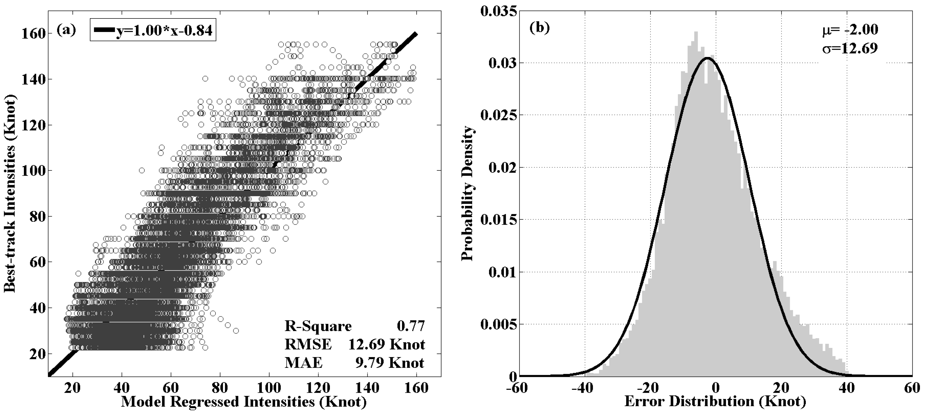
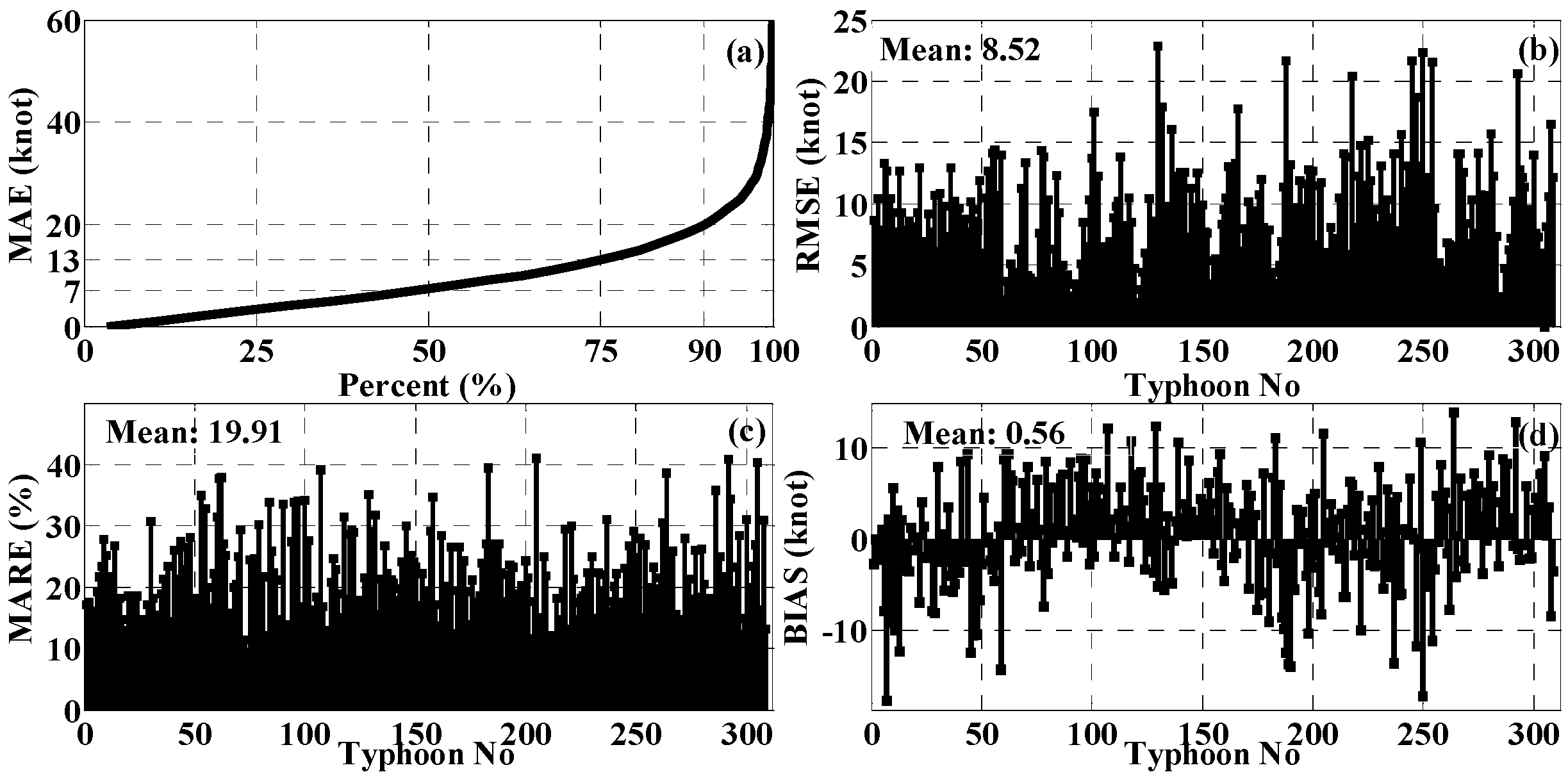
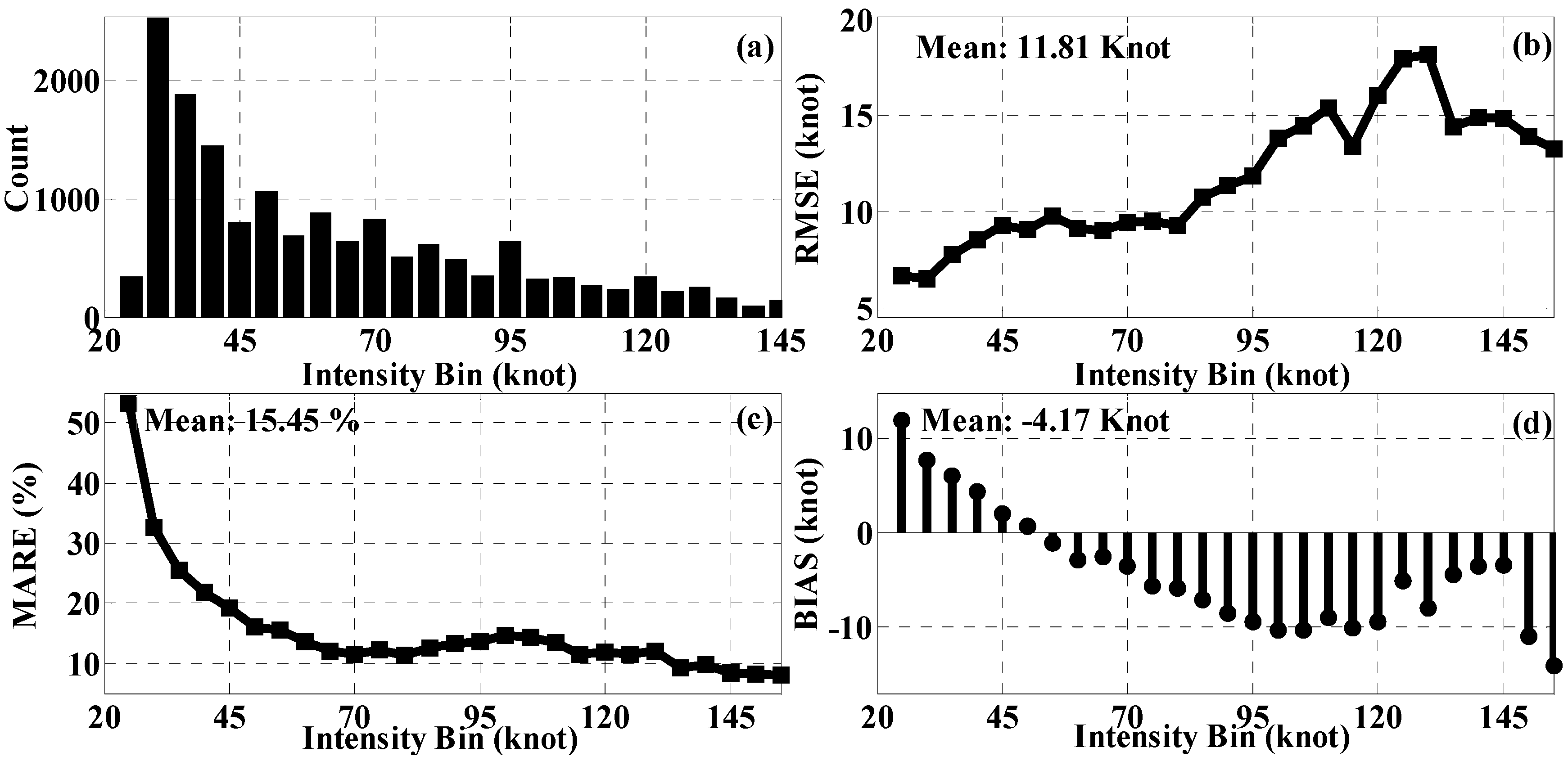
4.1. Dependent Tests and Results
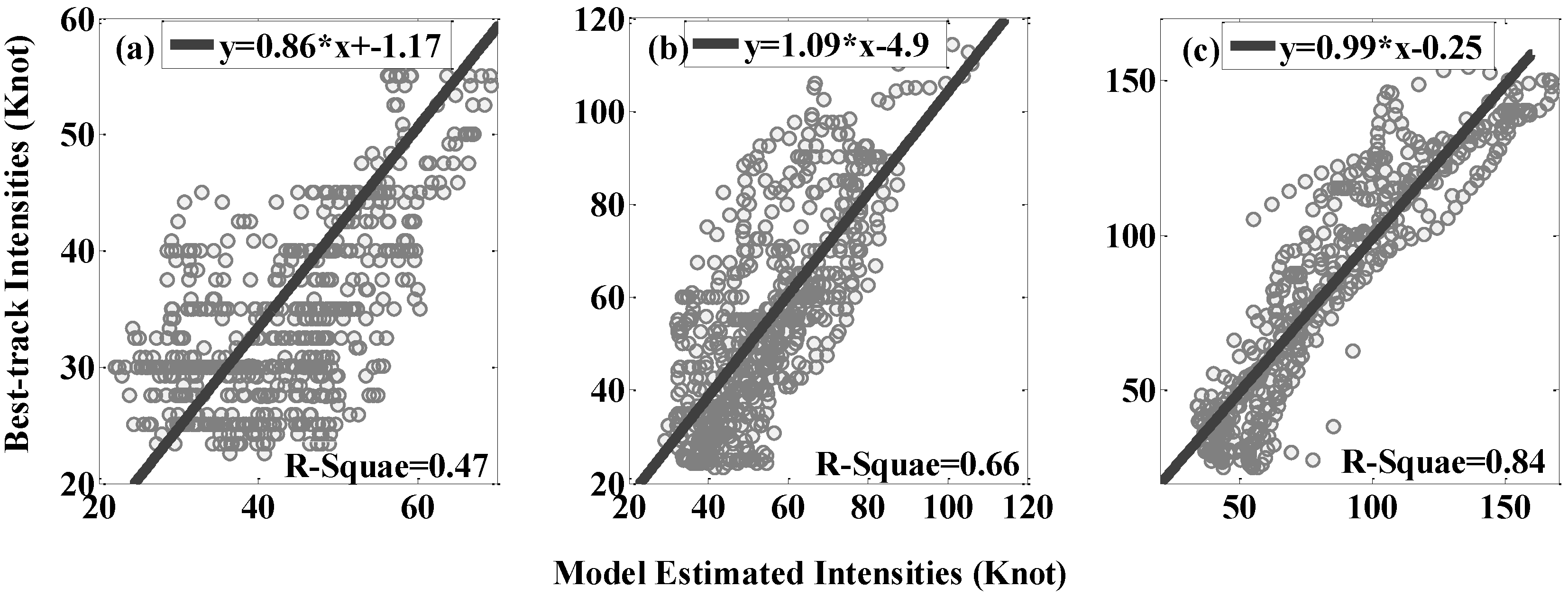
4.2. Independent Tests Results
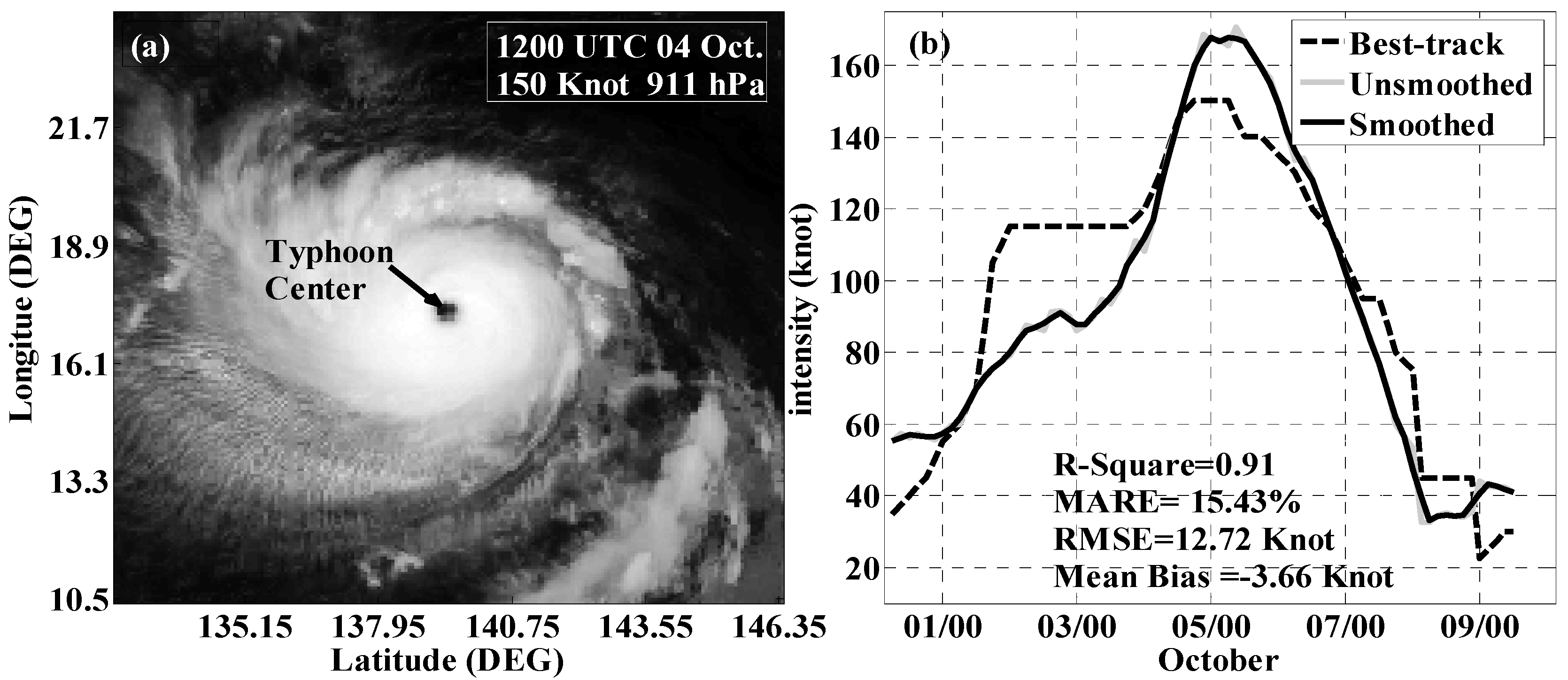
4.3. Case Analysis of Extreme Typhoon Melor (No. 202009)
5. Conclusions
Acknowledgments
Author Contributions
Conflicts of Interest
Abbreviations
| TC | Tropical Cyclone |
| BT | Brightness Temperature |
| NWP | Northwestern Pacific Ocean |
| TCIS | The JPL Tropical Cyclone Information System |
| GMS | Geostationary Meteorological Satellite |
| IRBT | Infrared Brightness Temperature |
| MSW | Maximum Sustained Wind |
| JTWC | National Joint Typhoon Warning Center |
| DAV | The Variance of Deviation Angles |
| DAV-T | The Deviation-Angle Variance Technique |
| P_MDA | The Probability Density of Mean Deviation Angle |
| IQR | Interquartile Range of the DAs |
| ICBT | The Inner Core Average BT |
| OCBT | The Outer Core Average BT |
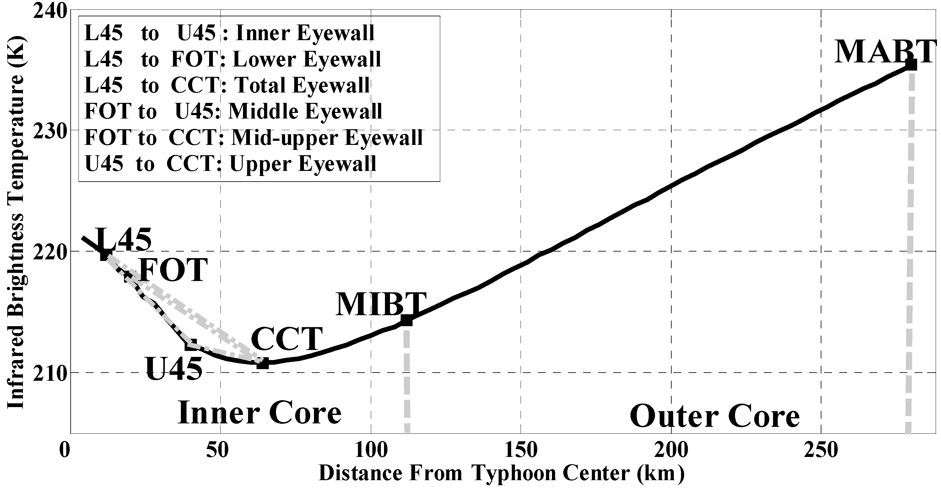
| MIBT (MABT) | Azimuthally Averaged Minimum (Maximum) BT within the Outer Core |
| CCT | The Radial Location of the Coldest Cloud |
| FOT | The Radial Location of the First Overshooting Top |
| L45 (U45) | The Lower (Upper) Extent of the Inner Eyewall |
| MAE | Mean Absolute Error |
| RMSE | Root Mean Square Error |
| MARE | Mean Absolute Relative Error |
References
- Tang, D.L.; Sui, G.; Lavy, G.; Pozdnyakov, D.; Song, Y.T.; Switzer, A.D. Typhoon Impact and Crisis Management; Springer: New York, NY, USA, 2014. [Google Scholar]
- Liu, C.-C.; Shyu, T.-Y.; Chao, C.-C.; Lin, Y.-F. Analysis on typhoon longwang intensity changes over the ocean via satellite data. J. Mar. Sci. Technol. 2009, 17, 23–28. [Google Scholar]
- Zhuge, X.-Y.; Guan, J.; Yu, F.; Wang, Y. A new satellite-based indicator for estimation of the western North Pacific tropical cyclone current intensity. IEEE Trans. Geosci. Remote Sens. 2015, 53, 5661–5676. [Google Scholar] [CrossRef]
- Velden, C.S.; Goodman, B.M.; Merrill, R.T. Western North Pacific tropical cyclone intensity estimation from noaa polar-orbiting satellite microwave data. Mon. Weather Rev. 1991, 119, 159–168. [Google Scholar] [CrossRef]
- Brueske, K.F.; Velden, C.S. Satellite-based tropical cyclone intensity estimation using the NOAA-KLM series Advanced Microwave Sounding Unit (AMSU). Mon. Weather Rev. 2003, 131, 687–697. [Google Scholar] [CrossRef]
- Aberson, S.D.; Black, M.L.; Black, R.A.; Cione, J.J.; Landsea, C.W.; Marks, F.D., Jr.; Burpee, R.W. Thirty years of tropical cyclone research with the NOAA P-3 aircraft. Bull. Am. Meteorol. Soc. 2006, 87, 1039–1055. [Google Scholar] [CrossRef]
- Kossin, J.P.; Knaff, J.A.; Berger, H.I.; Herndon, D.C.; Cram, T.A.; Velden, C.S.; Murnane, R.J.; Hawkins, J.D. Estimating hurricane wind structure in the absence of aircraft reconnaissance. Weather Forecast. 2007, 22, 89–101. [Google Scholar] [CrossRef]
- Knaff, J.A.; Longmore, S.P.; DeMaria, R.T.; Molenar, D.A. Improved tropical-cyclone flight-level wind estimates using routine infrared satellite reconnaissance. J. Appl. Meteorol. Climatol. 2015, 54, 463–478. [Google Scholar] [CrossRef]
- Velden, C.; Harper, B.; Wells, F.; Beven, J.L.; Zehr, R.; Olander, T.; Mayfield, M.; Guard, C.C.; Lander, M.; Edson, R. The dvorak tropical cyclone intensity estimation technique: A satellite-based method that has endured for over 30 years. Bull. Am. Meteorol. Soc. 2006, 87, 1195–1210. [Google Scholar] [CrossRef]
- Chao, C.-C.; Liu, G.-R.; Liu, C.-C. Estimation of the upper-layer rotation and maximum wind speed of tropical cyclones via satellite imagery. J. Appl. Meteorol. Climatol. 2011, 50, 750–766. [Google Scholar] [CrossRef]
- Sadler, J.C. Tropical cyclones of the Eastern North Pacific as revealed by TIROS observations. J. Appl. Meteorol. 1964, 3, 347–366. [Google Scholar] [CrossRef]
- Hubert, L.F.; Timchalk, A. Estimating hurricane wind speeds from satellite pictures. Mon. Weather Rev. 1969, 97, 382–383. [Google Scholar] [CrossRef]
- Dvorak, V.F. Tropical Cyclone Intensity Analysis Using Satellite Data; US Department of Commerce, National Oceanic and Atmospheric Administration, National Environmental Satellite, Data, and Information Service: Washington, DC, USA, 1984.
- Dvorak, V.F. Tropical cyclone intensity analysis and forecasting from satellite imagery. Mon. Weather Rev. 1975, 103, 420–430. [Google Scholar] [CrossRef]
- Velden, C.S.; Olander, T.L.; Zehr, R.M. Development of an objective scheme to estimate tropical cyclone intensity from digital geostationary satellite infrared imagery. Weather Forecast. 1998, 13, 172–186. [Google Scholar] [CrossRef]
- Piñeros, M.F.; Ritchie, E.A.; Tyo, J.S. Estimating tropical cyclone intensity from infrared image data. Weather Forecast. 2011, 26, 690–698. [Google Scholar] [CrossRef]
- Olander, T.L.; Velden, C.S.; Turk, M.A. Development of the Advanced Objective Dvorak Technique (AODT)—Current progress and future directions. In Proceedings of the 25th Conference on Hurricanes and Tropical Meteorology, San Diego, CA, USA, 29 April–3 May 2002.
- Olander, T.L.; Velden, C.S. The advanced dvorak technique: Continued development of an objective scheme to estimate tropical cyclone intensity using geostationary infrared satellite imagery. Weather Forecast. 2007, 22, 287–298. [Google Scholar] [CrossRef]
- Mueller, K.J.; DeMaria, M.; Knaff, J.; Kossin, J.P.; Vonder Haar, T.H. Objective estimation of tropical cyclone wind structure from infrared satellite data. Weather Forecast. 2006, 21, 990–1005. [Google Scholar] [CrossRef]
- Fetanat, G.; Homaifar, A.; Knapp, K.R. Objective tropical cyclone intensity estimation using analogs of spatial features in satellite data. Weather Forecast. 2013, 28, 1446–1459. [Google Scholar] [CrossRef]
- Piñeros, M.F.; Ritchie, E.A.; Tyo, J.S. Objective measures of tropical cyclone structure and intensity change from remotely sensed infrared image data. IEEE Trans. Geosci. Remote Sens. 2008, 46, 3574–3580. [Google Scholar] [CrossRef]
- Ritchie, E.A.; Valliere-Kelley, G.; Piñeros, M.F.; Tyo, J.S. Tropical cyclone intensity estimation in the north Atlantic basin using an improved deviation angle variance technique. Weather Forecast. 2012, 27, 1264–1277. [Google Scholar] [CrossRef]
- Piñeros, M.F.; Ritchie, E.; Tyo, J.S. Detecting tropical cyclone genesis from remotely sensed infrared image data. IEEE Geosci. Remote Sens. Lett. 2010, 7, 826–830. [Google Scholar] [CrossRef]
- Rodríguez-Herrera, O.G.; Wood, K.M.; Dolling, K.P.; Black, W.T.; Ritchie, E.; Tyo, J.S. Automatic tracking of pregenesis tropical disturbances within the deviation angle variance system. IEEE Geosci. Remote Sens. Lett. 2015, 12, 254–258. [Google Scholar] [CrossRef]
- Ritchie, E.A.; Wood, K.M.; Rodríguez-Herrera, O.G.; Piñeros, M.F.; Tyo, J.S. Satellite-derived tropical cyclone intensity in the north pacific ocean using the deviation-angle variance technique. Weather Forecast. 2014, 29, 505–516. [Google Scholar] [CrossRef]
- Liu, C.-C.; Liu, C.-Y.; Lin, T.-H.; Chen, L.-D. A satellite-derived typhoon intensity index using a deviation angle technique. Int. J. Remote Sens. 2015, 36, 1216–1234. [Google Scholar]
- Hristova-Veleva, S.M. Using the JPL tropical cyclone information system for research and applications. In Proceedings of the 28th Conference on Hurricanes and Tropical Meteorology, Orlando, FL, USA, 28 April–2 May 2008.
- Knosp, B.W. The JPL tropical cyclone information system: Design and implementation. In Proceedings of the 28th Conference on Hurricanes and Tropical Meteorology, Orlando, FL, USA, 28 April–2 May 2008.
- Knosp, B.; Ao, C.; Chao, Y.; Dang, V.; Garay, M.; Haddad, Z.; Hristova-Veleva, S.; Lambrigtsen, B.; Li, P.; Park, K. The JPL Tropical Cyclone Information System: Data and Tools for Researchers; AGU: San Francisco, CA, USA, 2008. [Google Scholar]
- Knapp, K.R.; Kossin, J.P. New global tropical cyclone data set from ISCCP b1 geostationary satellite observations. J. Appl. Remote Sens. 2007, 1, 013505–013506. [Google Scholar]
- Chu, J.-H.; Sampson, C.R.; Levine, A.S.; Fukada, E. The joint typhoon warning center tropical cyclone best-tracks, 1945–2000. Available online: http://www.usno.navy.mil/JTWC (accessed on 9 March 2016).
- Zhao, H.; Wu, L.; Wang, R. Decadal variations of intense tropical cyclones over the Western North Pacific during 1948–2010. Adv. Atmos. Sci. 2014, 31, 57–65. [Google Scholar] [CrossRef]
- Chan, J.C. Decadal variations of intense typhoon occurrence in the Western North Pacific. R. Soc. 2008, 464. [Google Scholar] [CrossRef]
- Zhao, H.; Wu, L.; Zhou, W. Interannual changes of tropical cyclone intensity in the Western North Pacific. J. Meteorol. Soc. Jpn. 2011, 89, 243–253. [Google Scholar] [CrossRef]
- Knaff, J.A.; Longmore, S.P.; Molenar, D.A. An objective satellite-based tropical cyclone size climatology. J. Clim. 2014, 27, 455–476. [Google Scholar] [CrossRef]
- Croxford, M.; Barnes, G.M. Inner core strength of atlantic tropical cyclones. Mon. Weather Rev. 2002, 130, 127–139. [Google Scholar] [CrossRef]
- Weatherford, C.L.; Gray, W.M. Typhoon structure as revealed by aircraft reconnaissance. Part I: Data analysis and climatology. Mon. Weather Rev. 1988, 116, 1032–1043. [Google Scholar] [CrossRef]
- Weatherford, C.L.; Gray, W.M. Typhoon structure as revealed by aircraft reconnaissance. Part II: Structural variability. Mon. Weather Rev. 1988, 116, 1044–1056. [Google Scholar] [CrossRef]
- Sanabia, E.R.; Barrett, B.S.; Fine, C.M. Relationships between tropical cyclone intensity and eyewall structure as determined by radial profiles of inner-core infrared brightness temperature. Mon. Weather Rev. 2014, 142, 4581–4599. [Google Scholar] [CrossRef]
- Olander, T.L.; Velden, C.S. Tropical cyclone convection and intensity analysis using differenced infrared and water vapor imagery. Weather Forecast. 2009, 24, 1558–1572. [Google Scholar] [CrossRef]
- Hazelton, A.T.; Hart, R.E. Hurricane eyewall slope as determined from airborne radar reflectivity data: Composites and case studies. Weather Forecast. 2013, 28, 368–386. [Google Scholar] [CrossRef]
- Kossin, J.; Knapp, K.; Vimont, D.; Murnane, R.; Harper, B. A globally consistent reanalysis of hurricane variability and trends. Geophys. Res. Lett. 2007, 34. [Google Scholar] [CrossRef]
- Lajoie, F.; Walsh, K. A technique to determine the radius of maximum wind of a tropical cyclone. Weather Forecast. 2008, 23, 1007–1015. [Google Scholar] [CrossRef]


| Bins | No. and Percent of Images in Training Dataset | No. and Percent of Images in Validation Dataset |
|---|---|---|
| Tropical Depression | 4752 (29.47%) | 581 (29.31%) |
| Tropical Storm | 5513 (34.19%) | 707 (35.67%) |
| C1 (Typhoon) | 2444 (15.16%) | 214 (10.80%) |
| C2 (Moderate Typhoon) | 1522 (7.70%) | 142 (7.16%) |
| C3 (Severe Typhoon) | 910 (5.64%) | 325 (5.75%) |
| C4 (Super Typhoon) | 1041 ( 6.46%) | 160 (8.07%) |
| C5 (Extreme Typhoon) | 252 (1.39%) | 46 (2.32%) |
| Overall | 16,126 (100%) | 1982 (100%) |
| Potential Predictors | Description |
|---|---|
| ICBT | Average BT within the inner core (0°–1° radially) |
| OCBT | Average BT within the outer core (1°–2.5° radially) |
| MIBT | Azimuthally averaged minimum BT within the outer core |
| MABT | Azimuthally averaged maximum BT within the outer core |
| SL45-FOT | The slope of the lower eyewall |
| SL45-U45 | The slope of the inner eyewall |
| SL45-CCT | The slope of the total eyewall |
| SFOT-U45 | The slope of the middle eyewall |
| SFOT-CCT | The slope of the mid-upper eyewall |
| SU45-CCT | The slope of the upper eyewall |
| AL45-FOT | The average BT within the lower eyewall |
| AL45-U45 | The average BT within the inner eyewall |
| AL45-CCT | The average BT within the total eyewall |
| AFOT-U45 | The average BT within the middle eyewall |
| AFOT-CCT | The average BT within the mid-upper eyewall |
| AU45-CCT | The average BT within the upper eyewall |
| Predicators | Added Order | Coefficients | p-Value | RMSE after Addition of the Predicator (Knot) | Coefficients for Normalized Predicators | Relative Contribution (%) |
|---|---|---|---|---|---|---|
| DAV2 | 1st | −6.04 × 10⁻⁶ | 3.39 × 10−61 | 31.11 | −22.37 | 1.66 |
| DAO | 2nd | 44.64 | 4.35 × 10−115 | 19.41 | 43.69 | 3.24 |
| ICBT/AL45-U45 | 3rd | −2703.25 | 0 | 17.22 | −565.05 | 41.92 |
| ICBT/AFOT-U45 | 4th | 2730.51 | 0 | 16.46 | 543.39 | 40.31 |
| SL45-U45 | 5th | 12.81 | 4.90 × 10−112 | 15.46 | 84.61 | 6.28 |
| OCBT/AL45-FOT | 6th | −201.98 | 3.46 × 10⁻³³ | 13.16 | −57.45 | 4.26 |
| OCBT/AU45-CCT | 7th | 126.48 | 1.42 × 10⁻¹⁶ | 12.69 | 31.34 | 2.32 |
| Bins | No. of Samples (%) | No. of Overestimated (%) | No. of Underestimated (%) | RMSE (Knot) | MARE (%) |
|---|---|---|---|---|---|
| Tropical Depression | 4752 (29.47) | 4597(96.74) | 155 (3.26) | 7.77 | 30.35 |
| Tropical Storm | 5513 (34.19) | 3575 (64.85) | 1938 (35.15) | 9.95 | 18.46 |
| C1 (Typhoon) | 2444 (15.16) | 766 (31.34) | 1678 (68.66) | 10.52 | 12.71 |
| C2 (Moderate Typhoon) | 1242 (7.70) | 397 (31.96) | 845 (68.04) | 12.94 | 14.79 |
| C3 (Severe Typhoon) | 910 (5.64) | 247 (27.14) | 663 (72.86) | 15.68 | 14.26 |
| C4 (Super Typhoon) | 1041 (6.46) | 391 (37.56) | 650 (62.44) | 17.49 | 11.82 |
| C5 (Extreme Typhoon) | 224 (1.39) | 107 (47.76) | 117 (52.24) | 18.93 | 10.69 |
| Overall | 16,126 (100) | 9314 (57.76) | 6812 (42.24) | 12.69 | 19.78 |
| <60 Knot | 60–120 Knot | ≥120 Knot | Overall | |
|---|---|---|---|---|
| RMSE (knot) | 6.47 | 11.22 | 12.29 | 12.01 |
| MAE (knot) | 8.30 | 8.92 | 9.47 | 9.50 |
| Mean Bias (knot) | 7.30 | 0.01 | 0.73 | 2.00 |
| MARE (%) | 26.34 | 18.76 | 15.16 | 21.67 |
| R2 | 0.47 | 0.66 | 0.84 | 0.77 |
| Dependent Tests | Independent Tests | |||
|---|---|---|---|---|
| Interpolated (16,126 Images) | Original (8652 Images) | Interpolated (1982 Images) | Original (931 Images) | |
| R2 | 0.77 | 0.78 | 0.77 | 0.81 |
| RMSE (Knot) | 12.69 | 9.88 | 12.01 | 9.48 |
| MARE (%) | 19.78 | 14.93 | 21.67 | 15.55 |
| Technique | RMSE (Knot) | |
|---|---|---|
| Kossin et al. (2007) | 13.20 | |
| Improved DAV-T | 12.90 | |
| TI index | 9.34 | |
| FASI | 12.70 | |
| Dependent test | Interpolated intensity | 12.69 |
| Original intensity | 9.88 | |
| Independent test | Interpolated intensity | 12.01 |
| Original intensity | 9.48 | |
© 2016 by the authors; licensee MDPI, Basel, Switzerland. This article is an open access article distributed under the terms and conditions of the Creative Commons by Attribution (CC-BY) license (http://creativecommons.org/licenses/by/4.0/).
Share and Cite
Zhao, Y.; Zhao, C.; Sun, R.; Wang, Z. A Multiple Linear Regression Model for Tropical Cyclone Intensity Estimation from Satellite Infrared Images. Atmosphere 2016, 7, 40. https://doi.org/10.3390/atmos7030040
Zhao Y, Zhao C, Sun R, Wang Z. A Multiple Linear Regression Model for Tropical Cyclone Intensity Estimation from Satellite Infrared Images. Atmosphere. 2016; 7(3):40. https://doi.org/10.3390/atmos7030040
Chicago/Turabian StyleZhao, Yong, Chaofang Zhao, Ruyao Sun, and Zhixiong Wang. 2016. "A Multiple Linear Regression Model for Tropical Cyclone Intensity Estimation from Satellite Infrared Images" Atmosphere 7, no. 3: 40. https://doi.org/10.3390/atmos7030040
APA StyleZhao, Y., Zhao, C., Sun, R., & Wang, Z. (2016). A Multiple Linear Regression Model for Tropical Cyclone Intensity Estimation from Satellite Infrared Images. Atmosphere, 7(3), 40. https://doi.org/10.3390/atmos7030040